Closing the ODE–SDE gap in score-based diffusion models through the Fokker–Planck equation
Teo Deveney, Jan Stanczuk, Lisa Kreusser, Chris Budd, Carola-Bibiane Schönlieb

TL;DR
This paper explains why ODE-based samplers in diffusion models perform worse than SDE-based ones and proposes a method to improve them using the Fokker–Planck equation.
Contribution
The paper introduces a theoretical framework linking ODE and SDE dynamics via the Fokker–Planck equation and proposes a regularization method to reduce their performance gap.
Findings
The difference between ODE and SDE samplers is linked to the Fokker–Planck residual.
Adding the Fokker–Planck residual as a regularization term improves ODE sampler performance.
Improving ODE samplers can sometimes degrade SDE sample quality.
Abstract
Score-based diffusion models have emerged as one of the most promising frameworks for deep generative modelling, due to both their mathematical foundations and their state-of-the art performance in many tasks. Empirically, it has been reported that samplers based on ordinary differential equations (ODEs) are inferior to those based on stochastic differential equations (SDEs). In this article, we systematically analyse the difference between the ODE and SDE dynamics of score-based diffusion models and show how this relates to an associated Fokker–Planck equation. We rigorously describe the full range of dynamics and approximations arising when training score-based diffusion models and derive a theoretical upper bound on the Wasserstein 2-distance between the ODE- and SDE-induced distributions in terms of a Fokker–Planck residual. We also show numerically that conventional score-based…
Genes, proteins, chemicals, diseases, species, mutations and cell lines named across the full text — each resolved to its canonical identifier and authoritative record.
Click any figure to enlarge with its caption.
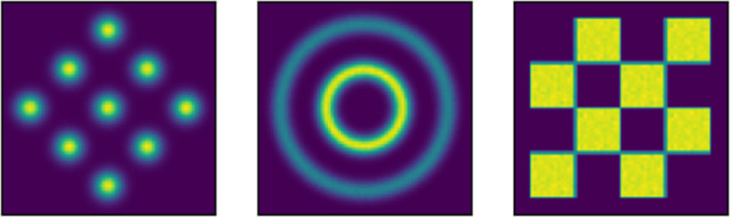 Figure 1
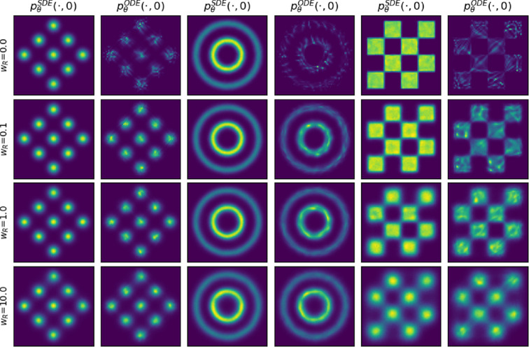 Figure 2
- —Engineering and Physical Sciences Research Councilhttp://dx.doi.org/10.13039/501100000266
- —Wellcome Trusthttp://dx.doi.org/10.13039/100010269
Peer Reviews
No public reviews on file for this paper yet. If you reviewed it on a platform where reviews are public (OpenReview, ICLR, NeurIPS, ICML), you can paste yours below so the community can read it here.
Videos
No videos yet. Explain this paper in a talk, walkthrough, or lecture? Add one.
Taxonomy
TopicsGenerative Adversarial Networks and Image Synthesis · Model Reduction and Neural Networks · Advanced Neuroimaging Techniques and Applications
Introduction
Generative modelling, the task of approximating the distribution underlying some given dataset, is useful in a range of scientific and non-scientific applications. The current state-of-the-art are diffusion models [1,2], which obtain this approximation by perturbing data with white noise and learning to iteratively denoise the perturbed data. Around the same time score-based models [3,4], which approximate the distribution through the gradient of its log-density (the score function), showed impressive results when combined with Langevin-based sampling. Today these frameworks have been unified into a single score-based diffusion approach [5], where stochastic differential equations (SDE) or ordinary differential equations (ODE) driven by score models are applied to denoise perturbed data. This has received a lot of attention from both theoretical and applied communities due its strong mathematical foundation and state-of-the-art performance [5,6]. In practice, differences between SDE and ODE-based sampling distributions are observed even for a common score model, thus motivating this work.
The SDE formulation arises from the conversion of data into noise through a diffusion process. As score-based diffusion is used for data generation, the time reversal of this process, i.e. the conversion from noise to data, is crucial and has a closed-form expression that depends on the (unknown) time-dependent score function of this diffusion. Hence, data generation is achieved by approximating these reverse dynamics through a neural approximation of the score function. The ODE framework, which originates from a diffusion-free reparameterization of the Fokker–Planck equation, offers a deterministic sampling method that offers significant theoretical and computational benefits such as tractable likelihood computation and access to more efficient ODE integrators for faster sample generation. However, the existing literature indicates that the ODE-based samplers are inferior to the SDE-based samplers in diffusion models. This is evidenced empirically in [5], reporting lower Fréchet inception distances (an image quality metric) for ODE-based samplers in their experiments. Moreover, theoretical analysis corroborates this observation, where tighter upper bounds have been derived for SDE-based sampling than for the ODE [7–11]. These discrepancies in performance raise questions about the validity of the likelihood computations attained in practice and prompt us to investigate the reasons for the discrepancy between SDE- and ODE-induced distributions.
In this article, we investigate the ODE–SDE gap in score-based diffusion models theoretically by analysing their connection to the mechanism underpinning their relationship—the Fokker–Planck equation. Our aim is to expose the theoretical insight that the ODE–SDE gap is related to how well the score model approximates the solution to a Fokker–Planck equation. As such, our work makes use of tools from the analysis of partial differential equations (PDEs), combined with methods for ODEs and SDEs. In addition, we provide numerical experiments using the Fokker–Planck equation to construct a regularizer. For toy examples in two dimensions, we attain explicit visual comparisons of the distributions generated by ODE and SDE samples and measure the relevant Wasserstein distances. We emphasize that the objective of our numerics is to accurately support our theory in an interpretable way. Since our approach to the numerics is more costly than a traditional diffusion model to train (though the cost of sampling from the trained model is unchanged), it is not proposed to be a scalable approach to training high-dimensional models, and we refer to [12] for more scalable approximate approaches in this direction.
Related work
(a)
The deterministic ODE dynamics for score-based diffusion models were introduced in [5]. To compare the ODE and SDE distributions, the authors in [5] show that under a perfect score approximation, the SDE and ODE distributions coincide and derive a method for computing the likelihoods based on the ODE formulation. In the same work, it is empirically reported that the ODE sampler exhibits inferior performance. This empirical finding highlights the necessity for a more rigorous theoretical investigation into this phenomenon. In [13], the authors bound the Kullback–Leibler divergence between the SDE-induced model distribution and the target true distribution in terms of the score-matching objective minimized during training. However, they also point out that the same bound does not hold for the ODE-induced distribution.
This issue is further explored in [14], where the authors introduce a new equality that can be used for bounds of the Kullback–Leibler divergence between the ODE-induced distribution and the data-generating distribution. Their findings reveal that the conventional score matching objective, typically employed in score-based diffusion models, fails to adequately control the error in the ODE distribution, and an alternative objective is proposed.
Since then, both the ODE and SDE formulation have been analysed. For SDE-based sampling, theoretical convergence guarantees including polynomial-in-time convergence under an score approximation have been proven [7–11]. For ODE-sampling, fast convergence (polynomial-in-time) has only been shown with the presence of Langevin-based correction steps [15]. Unfortunately, this approach results in a stochastic sampler that sacrifices deterministic mappings and is unsuitable for likelihood computations. The analysis of the fully deterministic system includes [16], which establishes an upper bound based on the number of steps of the discretized ODE. In addition, [17] provides error bounds for the flow matching method introduced in [18], a generalization of diffusion-based ODE methods. Of these works, the bound in [17] looks most similar to ours, though none are directly applicable to our setting, since they are all comparisons to the ground truth given in terms of an score approximation, whereas we investigate the ODE–SDE gap in terms of a Fokker–Planck residual.
More closely related to our work, the authors in [12] relate the Kullback–Leibler divergence between ODE-induced and data-generating distributions to the error in the Fokker–Planck equation associated with the diffusion process. They demonstrate that the residual of the Fokker–Planck equation can bound the ODE sample error up to some non-zero threshold. For full convergence, their analysis additionally requires minimization of the score-matching objective.
Our work shares some themes with [12], since we also consider the Fokker–Planck equation underlying the diffusion dynamics. However our focus here differs, as we specifically focus on the ODE–SDE gap. Moreover, our analysis has been conducted independently using a different theoretical toolbox, and this reveals different insights as highlighted in §1b.
Contributions
(b)
In this work, we provide a concise and rigorous exposition of the full range of densities and their approximations that arise in the score-based diffusion framework. This includes densities of the true and approximate dynamics—both deterministic and stochastic, as well as forward and backwards in time—with their density evolution equations and the neural approximations producing them. Given these dynamics, the contributions of this work are the following:
—We derive an upper bound between the densities induced by the approximate ODE and the approximate SDE. To the authors’ knowledge, this is the first such bound that does not relate each approximated density to the true one. The distance is key when querying both the ODE and the SDE of the same model, for example when stochastic sampling is combined with likelihood evaluations.
- —Our bound is in Wasserstein-distance, in contrast to previous works that mostly focus on weaker distances such as Kullback–Leibler divergence or total variation.
- —Our bound relates the distributions through the Fokker–Planck equation of the generative process. This distinguishes our work from prior works in the area and is the pertinent object to study since ODE-based sampling arises through a reformulation of the Fokker–Planck equation. We show that the ODE–SDE gap increases when the neural approximation fails to satisfy a Fokker–Planck equation.
- —We prove our result for both the potential parameterization, and the score parameterization more commonly used in practice, by considering the analogous Fokker–Planck equation for the score function. —We support our theory by providing numerical experiments using the residual of the Fokker–Planck equation in a regularization term. We visualize the densities and calculate the relevant Wasserstein distances to explicitly demonstrate that a lower residual error in the Fokker–Planck equation is associated with a lower ODE–SDE gap.
Outline
(c)
In §2, we describe the broad range of dynamics and approximations that arise when training a score-based diffusion model. Our main theoretical result on the ODE–SDE gap in score-based diffusion models is proven in §3, where we derive an upper bound on the Wasserstein 2-distance between the ODE- and SDE-induced distributions in terms of a Fokker–Planck residual. In §4, we provide numerical evidence showing explicitly that conventional score-based diffusion models can exhibit significant differences between SDE- and ODE-induced distributions. Moreover, we show that reducing the Fokker–Planck residual by adding it as an additional regularization term indeed leads to closing the gap between SDE and ODE distributions.
Score-based diffusion models
Assumptions and notation
(a)
We will work in the time domain for some and spatial domain . For two vectors , we denote their inner product , with associated norm . For a function , we denote the -norm over some domain as . We denote by the (spatial) gradient and by the Laplacian. For two probability measures, on , we denote their Wasserstein 2-distance by .
Let be a probability space and let be the natural filtration (the increasing family of sub- -algebras containing information at times ). As is convention, we denote by a Brownian motion at time with values in adapted to the filtration . Conversely, let denote a reverse filtration (the decreasing family of sub- -algebras containing information at times ). We denote by a Brownian motion at time with values in adapted to . Under suitable assumptions, SDEs driven by are adapted to , and SDEs driven by are adapted to . Throughout we will refer to the former as forward SDEs, and the latter as reverse SDEs even though both SDEs will initially be formulated using the forward time variable . When dealing with SDEs and the associated Fokker–Planck equations, we will distinguish between evolution equations running forward and backwards in time by introducing the reverse time variable to specify that the corresponding dynamics are in reverse time. We will denote the SDE dynamics parameterized with the forward and reverse time variables and by and , respectively, with . For any function , we introduce by for all . Further, let probability densities on be given, and we denote the associated log-densities by , on . Throughout the article, we make the following regularity assumptions:
Assumptions 2.1. Let and let such that for some . Assume that and there is such that for all . We assume that is a bounded domain with . For neural approximations, we assume smooth activation functions, so that neural potential models are in throughout, and neural score models are in . Moreover, we assume that there are such that and . Finally, we assume that the second moments of and are finite, and that .
Particle dynamics
(b)
We introduce the forward SDE as
equipped with some initial distribution for . In generative modelling settings, this initial distribution represents the underlying target distribution from which the data were sampled. In equation (2.1), denotes the value of a Brownian motion adapted to , and therefore is also adapted to . We denote the associated marginal density of samples from equation (2.1) at time by with . Note that equation (2.1) has a unique -continuous solution by assumptions 2.1.
In [19], the author shows that the process in equation (2.1) can be written as an SDE measurable with respect to the reverse filtration . We refer to this SDE as the reverse SDE, and it is given by
where is a Brownian motion adapted to at time . Intuitively, one can think of as the backwards evolution of Brownian motion with known terminal state, and equation (2.2) as the backwards evolution of equation (2.1). Accordingly, if the terminal distribution for is set to , then the trajectories of equation (2.2) share the same distribution as equation (2.1) for any time . As shown in [5], a reformulation of the Fokker–Planck equations allows us to derive the probability flow ODE of the forward SDE equation (2.1). This is given by
equipped with initial distribution for or, equivalently, terminal distribution for . The trajectories initialized from evolve forward in time according to equation (2.3) and also have marginal distribution at time . Similarly, the trajectories with terminal condition sampled from have marginal distribution at time . Therefore, we have that the associated densities toequations equations (2.1), (2.2) and (2.3) are all given by at any time .
Neural approximation
(c)
For generative tasks, practitioners assume to be equal to a given prior distribution and simulate equation (2.2) or (2.3) to generate samples from . Typically, approximates and is an easy to sample from distribution that contains no information of , such as a Gaussian distribution with fixed mean and variance. However, solving equation (2.2) or (2.3) requires knowledge of the (Stein) score function for any , which is not known in general and must be approximated from data. Therefore, a neural network with model parameters is trained to approximate the score function from the data by minimizing the weighted score matching objective:
where is a positive weighting function.
in equation (2.4) cannot be minimized directly since we do not have access to the ground truth score . Therefore, in practice, a different objective has to be used [3,5,20]. In [5], the weighted denoising score-matching objective is considered, which is defined as
The difference between equations equations (2.4) and (2.5) is the replacement of the unknown ground truth score by the score of the perturbation kernel , which can be determined analytically for many choices of forward SDEs. Note that for a fixed function , objective (2.5) is equal to objective (2.4) up to an additive constant, which does not depend on the model parameters . The reader can refer to [20] for the proof.
The choice of the weighting function determines the importance of score-matching at different noise scales. A principled choice is , known as the likelihood weighting due to its relation to likelihood-based training (see discussion in appendix E).
Most implementations of neural score approximations parameterize the time-dependent score vector field directly with a neural network on some bounded domain . Such approximations generally result in a non-conservative vector, which therefore cannot be a gradient field of any scalar field (see, for example, figure 5 in appendix D). Since we know a priori that the target vector field is a gradient field, instead of learning , we consider a neural network such that approximates the log-density for any up to some normalizing constant. In other words, there exists a (time-dependent) normalizing constant such that
is a probability distribution. We write for the induced log-density, and we call the function a potential model. During training, the induced approximate score is computed by back-propagation through with respect to the input . This results in a score approximation that is provably a conservative vector field. Moreover, it enables us to calculate the time derivative of the approximate log-density (up to normalization) as by back-propagation through with respect to , which will be convenient when we introduce and evaluate a log-Fokker–Planck residual for in §2f.
Approximate particle dynamics
(d)
The above neural approximations induce approximate versions of equation (2.2) and its deterministic flow equation (2.3). For ease of notation, we introduce the approximated reverse drift:
obtained by substituting the potential model into the drift of equation (2.2). Note that by the assumed properties of in assumptions 2.1, it follows that and . Using the approximated reverse drift equation (2.6) , we obtain the reverse approximate SDE:
which can be regarded as an approximation of equation (2.2). Here, is adapted to the reverse time filtration and by assumptions 2.1, equation (2.7) has a unique -continuous solution. We denote the marginal density of satisfying equation (2.7) by at time and equip it with some terminal distribution of at time , i.e. , where is chosen to be a Gaussian approximation of . Thus the accuracy of the reverse flow of probability induced by equation (2.7) depends on the accuracy of the potential model. Applying the result of [19] to write equation (2.7) as a process measurable with respect to , we arrive at the forward approximate SDE, given by
where is drawn from . The associated probability flow ODE of the approximate SDE (in forward time) is
where is drawn from . Note that the associated densities to equations (2.7), (2.8) and (2.9) are all given by for .
Finally, an approximation of the probability flow ODE equation (2.3) arises by approximating in equation (2.3) by a neural network . This yields the approximate probability flow ODE (in forward time):
using the approximate forward drift
Here, is distributed according to . We denote the associated density for .
In summary, the original formulations equations (2.1), (2.2) and (2.3) all have density , the approximations equations (2.7), (2.8) and (2.9) obtained by approximating the reverse SDE equation (2.2) all have density and the approximation of the probability flow ODE equation (2.3) has density . Moreover, there is a density implied directly by the neural approximation to log-density. In general, we have that .
For the majority of our calculations and numerics, it is more convenient to work with logarithms of densities rather than the densities themselves. For each density , we denote the associated log-density by and refer to as log-density or potential. That is, , , and for all .
In addition to considering the dynamics in forward time, we can also introduce the dynamics in reverse time. We denote the reverse time dynamics by for satisfying which implies that and for the initial and terminal conditions, respectively.
As we have a terminal condition for equation (2.7) and equation (2.7) is stated in forward time, the corresponding parameterization in reverse time can be useful for obtaining samples satisfying equation (2.7). It is given by
where we use the notation from §2a and the reverse time variable . We equip equation (2.12) with initial condition which is sampled from , and we denote the distribution of at time by . Note that for with . This implies that we can sample a particle from the target distribution by sampling from and solving equation (2.12) until time , for instance with the Euler–Maruyama scheme.
Similarly the ODE dynamics equation (2.10) can be written using the reverse time variable as
To sample from the approximate target distribution , sample an initial condition from and simulate equation (2.13) forward in time.
Fokker–Planck equations
(e)
The evolution of the densities subject to some initial or terminal condition are described by Fokker–Planck equations. For the forward SDE equation (2.1) the density obeys the forwardFokker–Planck equation:
on , equipped with the initial data on the full space . For our analysis, we restrict ourselves to a bounded domain with . For considering equation (2.14) on , we equip equation (2.14) with positive Dirichlet boundary conditions. Let denote a positive function that is equal to on . Note that we can assume without loss of generality that is positive on for . This yields the forward Fokker–Planck equation (2.14) on the domain with initial data restricted to and Dirichlet boundary conditions on . In addition, we set on .
The density of the approximate SDE equation (2.7) also satisfies a forward Fokker–Planck equation, which can be derived by writing the Fokker–Planck equation for the forward dynamics equation (2.8) of with appropriate terminal distribution. This gives the approximate Fokker–Planck equation (in forward time):
on , equipped with the terminal condition from assumptions 2.1 on the full space , i.e. for all , where is typically specified as a Gaussian approximation of . For considering equation (2.15) on a bounded domain , we introduce positive Dirichlet boundary conditions. Let denote a positive function that is equal to on . We obtain the approximate Fokker–Planck equation equation (2.15) on the domain with initial data restricted to and Dirichlet boundary conditions on . We set on .
Note that for , we always assume a fixed terminal condition at time when considering equation (2.15) in (or an initial condition when considering the evolution in reverse time ) as describes the flow of probability backwards from a Gaussian approximation of to some approximation of . Notice that equations (2.14) and (2.15) are of a similar form, apart from the different signs of the diffusion terms.
In addition to considering Fokker–Planck equations for the densities, one can also introduce log-Fokker–Planck equations for the potential. For the density satisfying the forward Fokker–Planck equation (2.14) for the forward SDE equation (2.1) and the associated potential we introduce the forward log-Fokker–Planck equation (in forward time) as
on . On the domain , we equip equation (2.14) with initial data restricted to and boundary conditions on .
For solving equation (2.15) in forward time, the log-density satisfies the approximate log-Fokker–Planck equation (in forward time) given by
on . On the domain , we again equip equation (2.17) with terminal data restricted to and boundary conditions on .
Fokker–Planck residuals
(f)
Our analysis in §3 is concerned with quantifying how the consistency of the neural approximation with the underlying Fokker–Planck equations is related to the ODE–SDE gap observed in practice. To measure this consistency, we derive a residual for the log-Fokker–Planck equation governing the evolution of the potential. In our theory, we use the residual as an error measure, and in our numerics, we add it as a regularization term to couple with the denoising score-matching objective in equation (2.5). Details on the implementation are given in §4.
Restricting ourselves to a bounded domain with , we consider a neural approximation with parameters , which learns the solution of the approximate log-Fokker–Planck equation (2.17) such that satisfies appropriate Dirichlet boundary conditions and terminal condition . This boundary condition ensures that the solution to equation (2.17) on Ω is everywhere equal to its corresponding solution on an unbounded domain.
Note that setting in equation (2.6) results in the probability flow ODE of the approximate SDE equation (2.9) (with density ) and approximate probability flow ODE equation (2.10) (with density ) coinciding. Thus, the gap between these two generative processes relates to the consistency of our neural approximation with the log-Fokker–Plank equation (2.17) associated with the approximate SDE. To measure the Fokker–Planck consistency, we substitute our model into equation (2.17) and measure the differential operator residual in the -norm. Manipulating this residual, we obtain
on . This demonstrates that the residual for the forward log-Fokker–Planck equation (2.16) is equivalent to the residual for the approximate log-Fokker–Planck equation (2.17) , thus it is sufficient to only consider the residual of the forward equation. Hence, we define the residual of the log-Fokker–Planck equation for the approximate reverse SDE equation (2.7) for any as
where is the volume of . We refer to as the log-Fokker–Planck residual. This residual quantifies how well our approximation agrees with the true solution to the approximate log-Fokker–Planck equation. In §3, we show how the values attained by this residual define an upper bound on the ODE–SDE discrepancy.
Note that analogous calculations hold for the residual in the standard Fokker–Planck equation (2.15) , and the score-Fokker–Planck equation discussed in §3c. In all cases, the residual corresponding to their forward Fokker–Planck equations is equal to the residual of the Fokker–Planck equation of the generative process, and these residuals relate to the ODE–SDE gap.
We remark that the bounded domain assumption made at the beginning of this subsection arises from the PDE analysis we apply to relate the neural approximation to the Fokker–Planck equation. This contrasts with other works deriving bounds for diffusion models since they do not investigate this relation, typically only considering generation under an -score approximation. In practice, this assumption is not restrictive, since for any data distribution and it is possible to choose a bounded domain such for all times . Therefore, the chance that a trajectory escapes this domain in practice is diminished.
Theoretical results on the ODE–SDE gap
In this section, we investigate the gap between the ODE- and SDE-induced distributions in terms of Fokker–Planck equations. More precisely, we derive bounds related to the approximate log-Fokker–Planck equation (2.17) in §3a, and in §3b we show that this theory applies to the associated potential model. In §3c, we provide a sketch of how to derive analogous bounds in terms of the approximate score-Fokker–Planck equation, thus addressing the common score parameterization. All these results are based on the following:
Assumptions 3.1. Let and be given, let be a bounded domain with . Assume that satisfies equation (2.15) on with terminal condition restricted to and Dirichlet boundary conditions on , with . Further, let be the probability density associated with equation (2.10) with terminal condition restricted to .
The ODE–SDE gap for the approximate Fokker–Planck equation
(a)
We show that, at a fixed time , satisfying the approximate Fokker–Planck equation equation (2.15) converges to the density of the approximate probability flow ODE equation (2.10) with respect to the Wasserstein 2-distance as the log-Fokker–Planck residual in equation (2.19) goes to zero
Theorem 3.1. Assume that assumptions 2.1 and 3.1 hold. Further, assume that the neural network is determined such that obeys the terminal condition restricted to and Dirichlet boundary conditions on , and in (2.19) satisfies . Then, for some constant independent of .
We provide the proof of theorem 3.1 in appendix A. The constant in theorem 3.1 depends on the time horizon as well as the Lipschitz constants of and . Details of these dependencies are specified in the proof.
The ODE–SDE gap for the potential model associated with the approximate Fokker–Planck equation
(b)
A key benefit of score-based models is that scores are agnostic to multiplicative scaling of the underlying density, implying known normalizing constants are not required for their implementation. So far, we have implicitly assumed that is an approximation of for a density , and hence that the integral of is normalized which is non-trivial in practice. To overcome this issue, we introduce an unnormalized network as a potential model and relate it to by introducing a (potentially time-varying) normalizing constant for . This gives the relation
which we also use to obtain the terminal data and boundary conditions on . The bounds on the ODE–SDE gap in theorem 3.1 also hold when considering instead of in the Fokker–Planck residual equation (2.19), as shown in appendix B.
The ODE–SDE gap for the approximate score-Fokker–Planck equation
(c)
In this work, we primarily focus on the underlying connection between the ODE, the SDE and Fokker–Planck equations observed in score-based diffusion models, and thus our focus has been on the potential parameterization discussed so far. However, in most practical implementations, a score parameterization is adopted due to computational efficiency, given by for the density and the log-density of the forward SDE equation (2.1). The score parameterization is linked to the score-Fokker–Planck equation, see e.g.[12]. To ensure applicability of our results to this case, we argue in this section that the bounds on the ODE–SDE gap in theorem 3.1 also hold for the score parameterization.
A score-Fokker–Planck equation can be derived by taking the gradient of the associated log-Fokker–Planck equation. To derive an analogous result to theorem 3.1, we are interested in the score-Fokker–Planck equation of the approximate SDE with log-Fokker–Planck equation (2.17) . Taking the gradient of equation (2.17) and setting yields the approximate score-Fokker–Planck equation:
Here, we use analogous notation to the potential case so that is the true score associated with the approximate reverse SDE equation (2.7) and is linked with the density via . Similarly, we also introduce the score associated with the approximate probability flow ODE equation (2.10). As before, we consider appropriate terminal data and Dirichlet boundary conditions.
Let denote a score model approximating . Following an analogous calculation to equation (2.18), the residual corresponding to the approximate score-Fokker–Planck equation (3.2) can be written as the residual of a score-Fokker–Planck equation, and we define the score-Fokker–Planck residual by
We can now state analogous result to theorem 3.1 for the score-Fokker–Planck equation:
Theorem 3.2. Assume that assumptions 2.1 and 3.1 hold. Further, assume that is determined such that and equipped with appropriate terminal and Dirichlet boundary conditions. Then, for some independent of .
Theorem 3.2 can be derived by applying analogous Steps I and II in the proof of theorem 3.1 and generalizing them to vector-valued functions as appropriate. More precisely, Step I of the proof has to be generalized to vector-valued solutions of equation (3.2) as opposed to the scalar solution of equation (2.17) but due to the similarity of the equations, this step can be done analogously. Step II follows as in the proof of theorem 3.1. Due to the similarity of the proofs, the detailed proof is omitted here.
Numerical experiments
To demonstrate our analytical results numerically and ensure visual interpretability, we implement several diffusion models in that attain a range of log-Fokker–Planck residual values (equation (2.19)) using various toy datasets. For the forward SDE, we choose and , resulting in the simple Ornstein–Uhlenbeck process Following equation (2.16), the associated log-Fokker–Planck equation is given by In our experiments, we take three different data distributions and train a neural network to minimize the loss function for differing values of , where and are defined in equations (2.5) and equation (2.19), respectively, and is set according to the likelihood weighting. Note that for our specific setting, we have
Therefore, both the denoising score matching objective and the log-Fokker–Planck residual are approximated using Monte Carlo estimation. We set and the likelihood weighting implies for . Note that we do not add terms that enforce boundary conditions in space or time, since the denoising score matching objective (2.5) already encourages consistency with these conditions (up to a multiplicative constant proportional to the underlying density). We generate samples from and using Euler–Maruyama and Euler discretizations of the reverse approximate SDE equation (2.7) and the reverse approximate probability flow ODE equation (2.10), respectively. To validate our results, we generate three million samples from each distribution. Due to computational constraints, these samples are then discretized on to a grid. When computing the Wasserstein distances to the target distribution and producing visualizations, we will consider the discretized distributions. Figure 1 shows the target distributions for our experiments.
Left to right our three examples are a Gaussian mixture, a concentric circles distribution and a checkerboard distribution.
We choose two-dimensional examples to ensure we can explicitly see the behaviour of the distributions and measure distances. Our examples cover the analytically solvable Gaussian mixture case, a smooth concentric circles distribution and a discontinuous checkerboard distribution to cover a range of scenarios of potential interest.
We parameterize our potential model by a fully connected neural network with two hidden layers of 80 nodes. We apply softplus activation functions, which have well defined first and second derivatives as required to evaluate . Each model is trained for 100 000 iterations using Adam with learning rate decaying from down to . Figure 2 shows the samples obtained from and for different weighting parameters .
Distributions of pθSDE(⋅,0) and pθODE(⋅,0) for weighting parameters wR taking values in (0,0.1,1,10) . The rows indicate which weighting parameter was used, while the columns indicate whether the displayed distribution is of pθSDE(⋅,0) or of pθODE(⋅,0) in the corresponding experiment. Samples displayed from the ODE and SDE samplers were attained using the same score model.
We see from figure 2 that if we only optimize (i.e. for ) the resulting is quite different from the true distribution. Notably, areas of high probability in do coincide with high probability regions of . Therefore in typical generative modelling scenarios, it may be difficult to identify this mischaracterization of the data distribution, given that individual samples generated from are generally plausible. Visually, we see that adding a factor of to the loss function initially results in an improvement in . The tables and figures inappendix C further detail these results. In table 2, we see that the distance between and consistently reduces for and when compared with , indicating an improvement in ODE samples. Increasing beyond this further reduces the gap between and as listed in table 1; however, this comes at the cost of increasing the distance from both and to which can be observed in tables 2 and 3 for . This can clearly be seen in figure 2 by the overly smoothed distributions that are attained with higher . Table 3 lists that the quality of degrades monotonically with increasing , which results in the negative correlation between and observed in figure 4. From this, we conclude that the cost of improving is a reduction in the quality of . Finally, in figure 3, we evaluate for each of our trained models and visualize the relation between and the associated values. This demonstrates a clear positive correlation supporting our theoretical analysis, where we proved an upper bound on the Wasserstein 2-distance between the ODE- and SDE-induced distributions in terms of a log-Fokker–Planck residual .
Conclusions
In this work, we conducted a systematic investigation into the dynamics that arise in score-based diffusion models. We mainly focused on the differences between the generative densities and defined by the reverse approximate SDE and the approximate probability flow ODE, respectively. Analytically, we proved that the discrepancy between and can be bounded by a log-Fokker–Planck residual in the Wasserstein 2-distance, thus giving a deeper insight into the connection between the two generative distributions in terms of the Fokker–Planck dynamics underlying the diffusion process. Numerically, we showed that and can differ substantially when the neural network is trained using the standard score-matching objective. Our numerical experiments also demonstrate that penalizing the loss function by the log-Fokker–Planck residual indeed leads to closing the gap between the ODE and the SDE distributions in the Wasserstein 2-distance. Our findings revealed that imposing this additional constraint within our loss function could improve the quality of when compared with the ground truth, though in exchange for this we observed concurrent degradation in the quality of . The practical implication of these findings is that enforcing self-consistency through penalization by the log-Fokker–Planck residual is unlikely to improve state-of-the-art generation using stochastic samplers. However, for downstream tasks where deterministic generation is required, such penalization could provide a potential avenue to improve sample quality and likelihood accuracy.
The reference list from the paper itself. Each links out to its DOI / PubMed record.
- 1Ho J , Jain A , Abbeel P . 2020 Denoising diffusion probabilistic models. Adv. Neural Inf. Process. Syst. 33 , 6840–6851.
- 2Sohl-Dickstein J , Weiss E , Maheswaranathan N , Ganguli S . 2015 Deep unsupervised learning using nonequilibrium thermodynamics (eds B Francis , D Blei ). In Proc. of the 32nd Int. Conf. on Machine Learning. Proc. of Machine Learning Research, vol. 37, pp. 2256–2265, Lille, France: PMLR.
- 3Hyvärinen A . 2005 Estimation of non-normalized statistical models by score matching. J. Mach. Learn. Res. 6 , 695–709.
- 4Song Y , Ermon S . 2019 Generative modeling by estimating gradients of the data distribution. In Proc. of the 33rd Int. Conf. on Neural Information Processing Systems. Red Hook, NY, USA: Curran Associates Inc.
- 5Song Y , Sohl-Dickstein J , P.Kingma D , Kumar A , Ermon S , Poole B . 2021 Score‑based generative modeling through stochastic differential equations. In 9th international conference on learning representations. Open Review.net. See https://openreview.net/forum?id=Px TIG 12RRHS.
- 6Dhariwal P , Nichol AQ . 2021 Diffusion models beat GA Ns on image synthesis. In Advances in neural information processing systems (eds M Ranzato , A Beygelzimer , Y Dauphin , PS Liang , J Wortman Vaughan ), pp. 8780–8794. Curran Associates, Inc. See https://proceedings.neurips.cc/paper_files/paper/2021/file/49ad 23d 1ec 9fa 4bd 8d 77d 02681 df 5cfa-Paper.pdf.
- 7Benton J , Bortoli DV , Doucet A , Deligiannidis G . 2024 Nearly d-linear convergence bounds for diffusion models via stochastic localization. In The twelfth international conference on learning representations. Vienna, Austria: Open Review.net. See https://openreview.net/forum?id=r 5nj V 3Bsu D.
- 8Chen S , Chewi S , Li J , Li Y , Salim A , Zhang A . 2023 Sampling is as easy as learning the score theory for diffusion models with minimal data assumptions. In The eleventh international conference on learning representations. Open Review.net. See https://openreview.net/forum?id=zy LV Mgs Z 0U\_.