Learning to estimate sample-specific transcriptional networks for 7,000 tumors
Caleb N. Ellington, Benjamin J. Lengerich, Thomas B. K. Watkins, Jiekun Yang, Abhinav K Adduri, Sazan Mahbub, Hanxi Xiao, Manolis Kellis, Eric P. Xing

TL;DR
This paper introduces a new method for estimating gene regulatory networks in tumors that accounts for individual differences and improves precision medicine by analyzing 7,000 tumors.
Contribution
The novel approach, contextualized network inference, uses multiview metadata to infer sample-specific gene regulatory networks and generalize to unseen cancer types.
Findings
Contextualized networks improve accuracy and identify additional prognostic tumor subtypes.
The method generalizes to unseen cancer types using a pan-cancer model of mutation effects on gene regulation.
A Python package and interactive tools are provided for learning and exploring contextualized models.
Abstract
Network estimation is essential for understanding the structure and function of biological systems, but current statistical approaches fail to capture intersubject heterogeneity or cross-modality information flow, both of which are needed for understanding complex phenotypes and pathologies. We introduce contextualized network inference, leveraging multiview contextual metadata to capture similarities and differences among heterogeneous observations during network estimation. Sharing information across contexts enables inference at sample-specific resolution, thus quantifying variation between subjects and revealing context-specific network rewiring. Applied to tumor-specific transcriptional network inference using clinical, molecular, and multiomic data, contextualized networks improve accuracy, generalize to unseen cancer types, and identify additional prognostic tumor subtypes. By…
Genes, proteins, chemicals, diseases, species, mutations and cell lines named across the full text — each resolved to its canonical identifier and authoritative record.
Click any figure to enlarge with its caption.
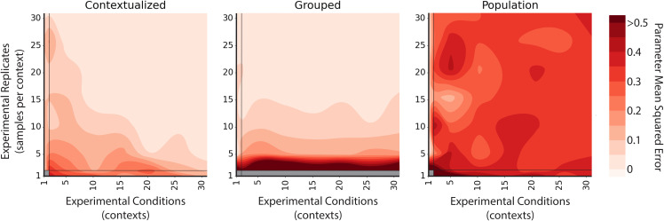 Fig. 2
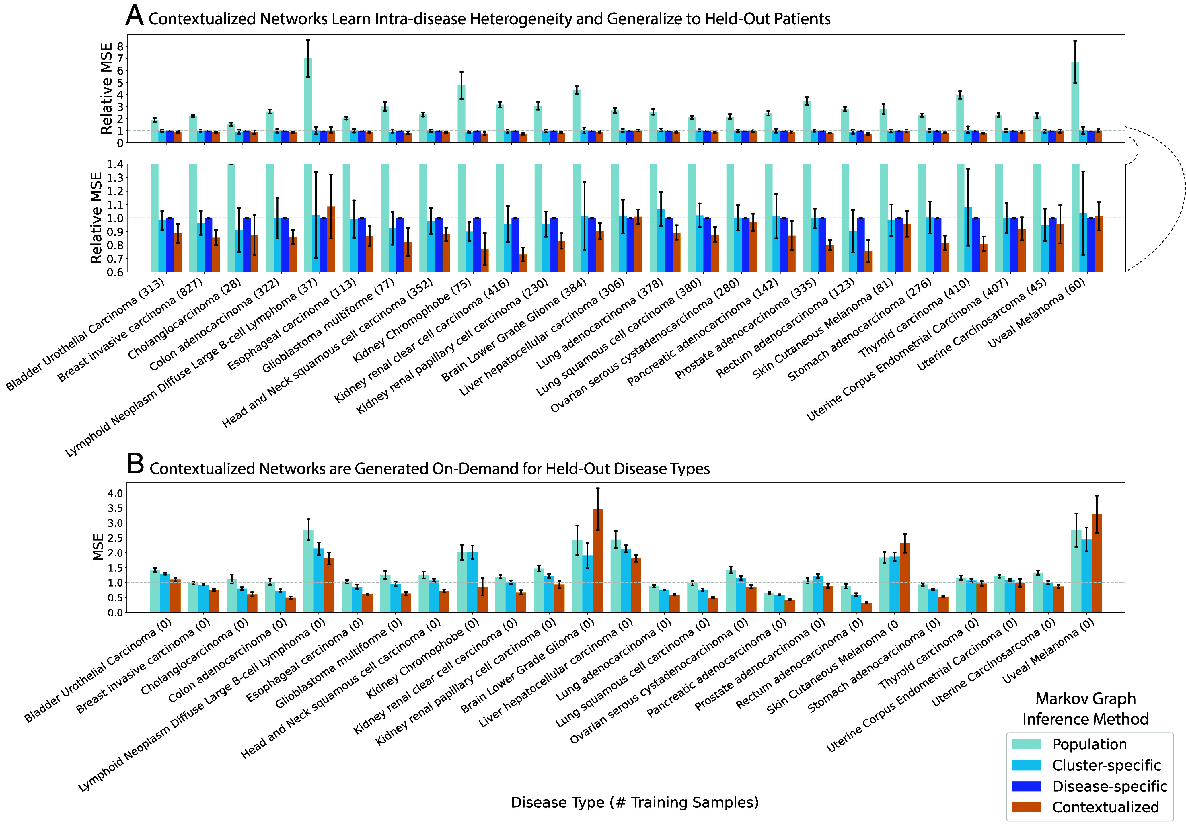 Fig. 3
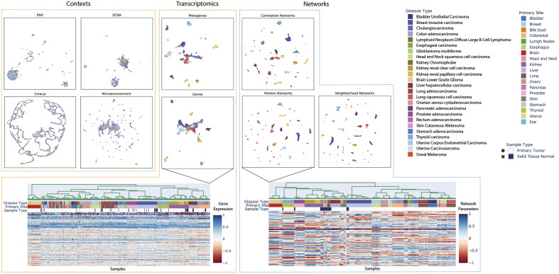 Fig. 4
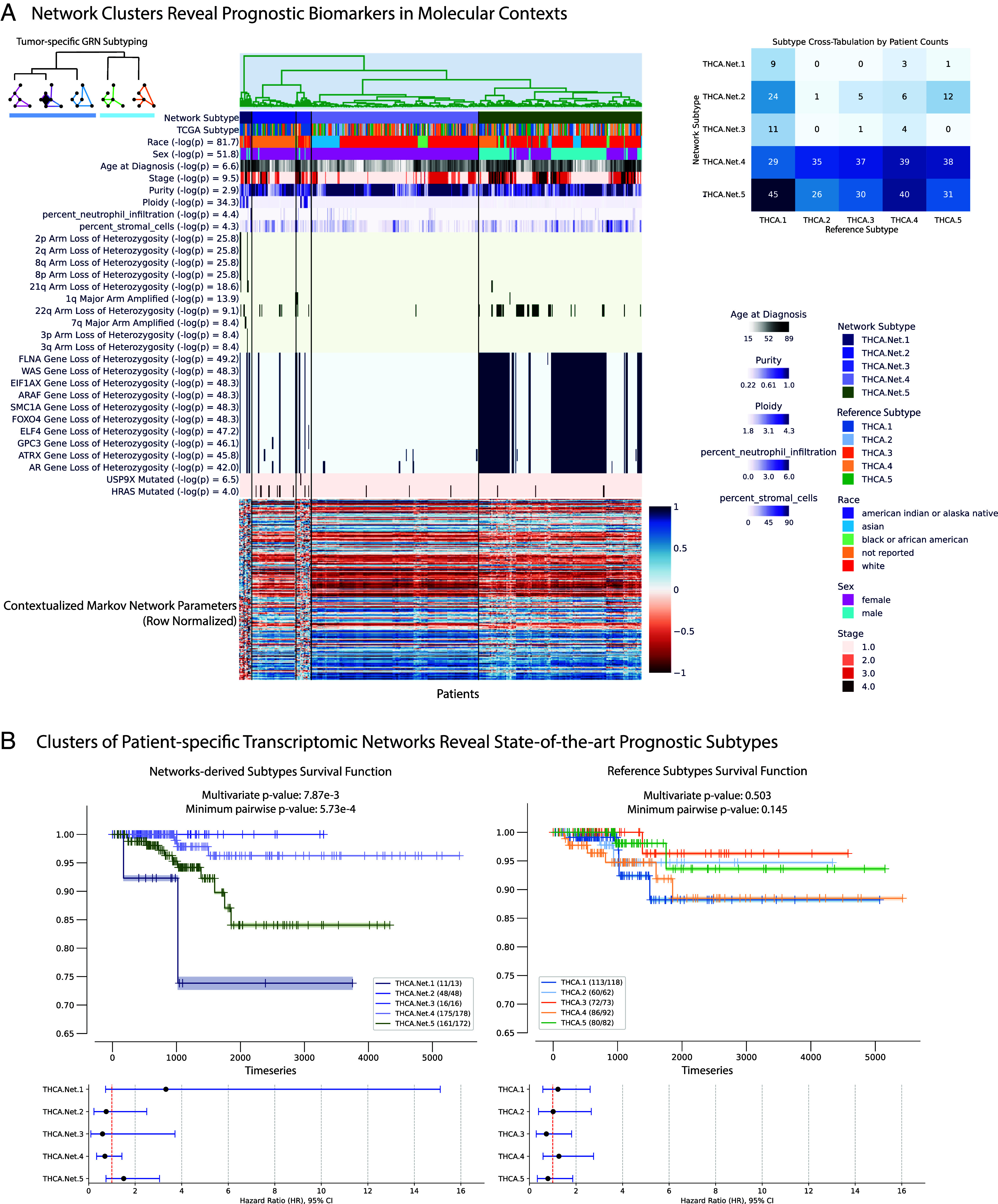 Fig. 5
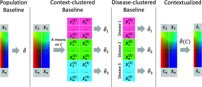 Fig. 6
| Markov | Neighborhood | Correlation | |
|---|---|---|---|
| Population |
|
|
|
| Cluster-specific |
|
|
|
| Disease-specific |
|
|
|
|
|
|
|
|
| Error Reduction |
|
|
|
| Average | Expression | Reference | Networks |
|---|---|---|---|
| Multivariate log-rank test | 8.53 | 9.65 |
|
| Minimum Pairwise log-rank test | 8.27 | 9.55 |
|
| Concordance Index | Expression | Reference | Networks |
|---|---|---|---|
| Patient average | 0.620 | 0.598 |
|
| Tissue average | 0.565 | 0.569 |
|
- —HHS | National Institutes of Health (NIH)100000002
Peer Reviews
No public reviews on file for this paper yet. If you reviewed it on a platform where reviews are public (OpenReview, ICLR, NeurIPS, ICML), you can paste yours below so the community can read it here.
Videos
No videos yet. Explain this paper in a talk, walkthrough, or lecture? Add one.
Taxonomy
TopicsGene expression and cancer classification · Bioinformatics and Genomic Networks · Cancer Genomics and Diagnostics
Tumors are heterogeneous, developing through clonal evolution that accumulates mutations, including cancer-driving single-nucleotide variants (SNVs) and somatic copy number alterations (SCNAs). In addition to tumor cell-intrinsic changes, tumors develop in and are shaped by a microenvironment that includes immune cells, the extracellular matrix, blood vessels, and surrounding cells. This extensive heterogeneity necessitates heterogeneous treatments targeted to individual patients. However, estimating treatment effects and patient prognosis at patient-specific resolution implies an n-of-1 approach to treatment that is technically and temporally infeasible. Instead, methods have historically sought to identify prognostic biomarkers that stratify patients into tumor subtype cohorts, and predictive biomarkers that identify patients who often respond to treatment. The Cancer Genome Atlas* (TCGA) derives prognostic subtypes via cluster analysis on clinical and molecular data, including cancer-driving SNVs, SCNAs, DNA methylation, mitochondrial DNA, RNA-seq, miRNA, protein abundance arrays, histology images, patient demographics, and/or immunological data, and further identifies prognostic biomarkers as features that differentiate these clusters (1???????????????????????–25). While clusters can be analyzed in terms of feature stratification, clustering ignores the latent feature interactions and hierarchical feature relationships that define biological systems. Biomarkers identified by cluster analysis have no mechanistic interpretation and require further experimentation to validate their role in tumorigenesis and tumor pathology. Consequently, the identification of biomarkers using somatic DNA alterations or gene expression patterns has proved challenging (26). Addressing the shortcomings of cluster analysis, we focus on three questions: 1) how do we model the mechanisms of molecular interactions as they relate to tumorigenesis and treatment efficacy, 2) how do we identify prognostic biomarkers for rare diseases and outlier patients that are too sparsely sampled to cluster, and 3) how can we quantify the heterogeneity of tumor pathology, which is widely acknowledged but poorly understood, and utilize multiview phenotypic, molecular, and environmental data to understand the forces driving heterogeneity?
GRNs help us to investigate these questions simultaneously. GRNs represent cellular circuitry, both responding to biomolecular stimulus and driving tumorigenesis. Interactions between disparate biomolecular entities can be identified at the cellular level through transcriptomic regulation, both directly and indirectly. In theory, tumor-specific GRNs capture regulatory redundancy and fragility in individual cancers. Relating tumor-specific GRNs to phenotypic, environmental, and multiomic features can reveal how these features relate to tumor pathology and the robustness of therapeutic targets GRN restructuring and reorganization. Single-cell and multiomic profiling have advanced the potential for studying highly context-specific regulatory relationships in GRNs, but computational methods of inferring GRNs continue to rely on partitioning samples into homogeneous sets of samples (27??–30). Partition-based modeling is insufficient to capture high-resolution or continuously rewiring GRNs, which is a problem for precision oncology because some types of cancer neither form discrete clusters (31) nor cluster by tissue of origin (32).
More generally, the increase of dataset complexity, heterogeneity, and size, has motivated the development of methods of “personalized” models across several application areas (33??–36). Personalized models seek to represent heterogeneous distributions as sample-specific distributions , where indexes a sample and corresponds to the sample-specific distribution. In the most difficult case of sample-specific inference, each is observed only a single time and hence information must be shared across samples.
Toward this aim of sharing information across samples, most personalized models make the simplifying assumption that all belong to the same family; i.e., . Through this lens of personalized modeling, understanding sample heterogeneity is reframed as estimating data distributions with sample-specific parameters. Some methods provide sample-specific estimators without additional information by imposing strong biological priors (37) or using a sample-left-out approach (38, 39), but these lack desirable properties such as the ability to generalize to new samples or even test model performance on held-out data. Due to the difficulty of estimating sample-specific parameters, most methods make use of side information (e.g., sample metadata) as a contextual representation of sample-to-sample variation (40???–44).
Given observations and contextual metadata , we have
where defines the context-specific model, and defines a context-specific density of model parameters , which we call the context encoder. One of the earliest ways to apply context encoding toward sample-specific parameter inference was the linear varying-coefficient (VC) model (44) in which linear regression parameters are predicted from context using a learned linear mapping or kernel density estimator. Extensions of this regime have been widespread (40?–42, 45), but typically focus on allowing models to vary over only a few continuous covariates (44?–46), or a small number of groups (40?–42)
Contextualized modeling (47, 48), combines the adaptability of VC models with the power of modern deep learning architectures by implementing the context encoder as a Dirac delta distribution defined by a deterministic deep neural network ,
thus benefiting from a wide range of architectures targeting high-dimensional and complex data types. When contexts are unique to each sample, the inferred models are sample-specific.
The contextualization framework also introduces the concept of model archetypes to combat the high-variance and uninterpretability of neural networks (Fig. 1D). All sample-specific models are spanned by the set of model archetypes, constraining and explaining their variation through the context encoding which parameterizes this space (Materials and Methods). These archetypes, also learned from data, link the heterogeneity of sample-specific models to variation in the context encoding and enable the sharing of information between sample-specific model inference tasks. This framework has been applied to estimating heterogeneous linear effects (47, 49?–51), but contextualized models have yet to be extended to the more general graphical modeling regime.
To infer tumor-specific GRNs that account for patient-to-patient heterogeneity, we propose to reframe GRN inference within the contextualized modeling paradigm (48), thereby sharing information among tumor-specific inference tasks by relating these tasks through their clinical and molecular contexts (Fig. 1). By recasting networks as the output of a learnable context encoder , our approach shares statistical power between samples while also permitting fine-grained variation to capture the complexity of sample-specific contexts such as tissue-of-origin, somatic mutation landscape, tumor microenvironment, and clinical measurements. We formulate three differentiable objectives for three types of GRNs (Markov, Neighborhood, and Correlation networks) under the contextualized modeling paradigm, and estimate sample-specific GRNs which enable sample-specific analyses of latent regulatory processes. We apply this computational framework to 7,997 tissue samples from TCGA, using bulk gene expression data as network samples , and immune cell infiltration metrics, patient demographics, and cancer-driver SCNAs and SNVs as context . We find that contextualized networks improve prediction of held-out expression data and reveal latent heterogeneity which has previously been obscured by partition-based methods of network inference.
Results
We introduce contextualized networks, which learn to personalize parametric network models based on context. This approach to network modeling enjoys two benefits over traditional network estimators: it scales across contexts to improve the accuracy of all networks as unique contexts are included, and it allows the incorporation of multiview context information to personalize the model. In studies on both simulated and real data, contextualized networks achieve high accuracy with as few as one training sample per context, while also generalizing to entirely unseen contexts. On real data, we apply contextualized networks to infer tumor-specific GRNs for 7,997 tumors, which learn to model the effect of individual clinical and molecular contexts on GRN structure and parameters, revealing latent GRN-based drivers of GRN dysregulation and tumor heterogeneity. We evaluate our 7997 tumor-specific GRNs for clinical and biological insights, identifying robust state-of-the-art prognostic subtypes for thyroid carcinoma. Finally, patient-specific networks relate prognostic biomarkers to changes in specific regulatory modules and gross GRN organization and identify candidate biomarkers for further investigation.
Unification of Markov, Correlation, and Neighborhood Network Objectives.
Statistical models for GRN inference can often be categorized as variants of four probabilistic models: Markov networks, which represent pairwise dependencies, Pearson’s correlation networks, which represent pairwise correlations, neighborhood selection networks, which represent each node as a linear combination of its neighbors, and Bayesian networks, and which represent directed and acyclic interactions. We focus on Markov, correlation, and neighborhood networks, unifying these models through linear reparameterization (Materials and Methods), thus enabling them to be contextualized uniformly with no change to the underlying contextualization framework.
Furthermore, linear parameterization gives a differentiable objective for optimizing each model, where the linear residual errors define mean-squared errors (MSEs) for measuring goodness-of-fit, which are also proportional to the negative log-likelihood of the data under the chosen network model (Materials and Methods). Beyond the modularity of this approach and its alignment with gradient-based optimization methods, MSEs enable benchmarking model performance in the absence of gold-standard networks with known structures. Thus, we enable quantitative comparison against baseline methods for network modeling even when tumor networks are too heterogeneous and individualized to determine gold-standard network structures.
Simulations.
The convergence rate of traditional network estimators is based on the number of experimental replicates, i.e., independent and identically distributed (i.i.d.) data draws. However, scaling within an i.i.d. domain is orthogonal to the goals of sample-specific modeling in heterogeneous regimes. Contextualization addresses this by providing a mechanism to scale model performance across data domains. In addition to the traditional route of increasing domain-specific or context-specific data collection, contextualization also scales performance with the total contexts available to the model, improving with the addition of unique experimental conditions. Arranged as axes, we describe these as “vertical” and “horizontal” scaling, respectively. We compare vertical and horizontal scaling properties of contextualized, context-grouped, and population model estimators by simulating known networks. We simulate a context-varying Gaussian, which allows us to control the number of samples per context and total contexts available to the model. Simulating Gaussians also allows us to evaluate the recovery of true parameters with our Gaussian-based network models.
Contextualized models are the only method capable of horizontal scaling, which drastically reduces the burden of vertical scaling (Fig. 2). With sufficient horizontal scaling, contextualized networks remain accurate even in sample-specific regimes and converge to true network parameters by learning to relate heterogeneous data through contextual metadata. However, with insufficient horizontal scaling, contextualized networks can be inferior to context-grouped or population modeling methods. For data domains with sample scarcity, contextualization presents an approach for improving model performance by sharing information across different contexts.
Error contours of Markov network estimators measured across experimental conditions (contexts) and experimental replicates (samples per context). Traditional estimators only scale vertically, improving error with experimental replicates or i.i.d. data draws. Modeling with heterogeneous or observational data requires estimators to scale horizontally, improving with more conditions or contexts. Contextualized modeling achieves this by learning to encode contextual information into model parameters. Population estimates a single model for all contexts, Grouped estimates a model for each context separately. Parameter MSE is taken between the predicted and ground truth precision matrices of the Markov networks and averaged over five bootstrapped runs.
Contextualized Networks Improve Likelihood of Held-Out Expression Profiles.
Contextualization improves the fit of network models to gene expression data (Table 1). We benchmark the contextualized networks by comparing them against several granularities of partition-based models: 1) a population network model that estimates the same network for all samples, 2) cluster-specific networks that are estimated independently for each cluster of contextual information, and 3) disease-specific networks that are estimated independently for each cancer type. For all three network models, we evaluate the fit of the network model to actual expression data. These predictive performances are measured as MSEs between predicted and observed expression data, a convenient result of our linearization and unification of correlation, Markov, and neighborhood selection objectives (Materials and Methods). Relative to disease-specific model inference (the best baseline method), contextualized networks reduce modeling error on average by 14.6% for Markov networks, 18.1% for neighborhood selection, and 20.2% for correlation networks. Contextualized networks achieve this improved predictive performance by accounting for contextual dependencies in model parameters without imposing prior assumptions on the form of these dependencies. As a result, contextualized graphical models capture highly localized and context-specific effects that can be overlooked by group-level modeling approaches (e.g., cluster-specific, disease-specific models).
Contextualized Networks Share Power Between All Cancer Types and Infer Models for Unseen Diseases.
Contextualization relates transcriptional regulation to genomic variation through a context encoder. During training, the encoder learns to modify the parameters of a downstream network model in response to contextual signals. At test time, the encoder uses learned context signals to generalize between sparsely sampled contexts. Splitting model performance by disease, contextualization sets a state-of-the-art on 22 of 25 disease types (Fig. 3A). Rare or undersampled diseases like kidney chromophobe and glioblastoma multiforme can especially benefit from contextual signals learned from well-sampled diseases in similar tissues. In disease-specific modeling, these smaller subpopulations must either be lumped within a larger tissue group, ignoring subpopulation heterogeneity, or modeled individually, sacrificing statistical power in a “large small ” regime. For example, there are training samples from kidney chromophobe patients, while each disease-specific network has edges, or parameters; estimating a disease-specific network from such limited data would be prohibitively high-variance for disease-specific modeling but is straightforward for contextualized networks.
Performance of Contextualized Markov Networks broken down by disease type. (A) Testing on a random split of held-out patients. MSE for Markov networks is defined in Materials and Methods. Relative MSE scales the MSEs of all models against the Disease-specific MSEs. (B) Disease-fold cross-validation, in which each of the 25 disease types is held out from training and evaluated only at testing time. We evaluate in terms of absolute MSEs, as Disease-specific network inference cannot be applied in this regime. Results are from 30 bootstrapped runs for each hold-out disease type and the hold-out patient set. Bar height is the disease-averaged error metric of the bootstrap-averaged network models. Error bars are the SD over bootstraps of the disease-averaged error metric of the network models.
Furthermore, contextualization adapts models to unseen contexts at test time, responding to even extreme distribution shift (Fig. 3B). For completely unseen contexts, the context encoder can still leverage learned relationships between contexts and models to infer zero-shot network models on demand. We evaluate model performance through a disease-fold cross-validation, where we hold out each of the 25 disease types in turn and learn to contextualize networks on the remaining 24. Notably, disease-specific modeling cannot be applied in this regime. In contrast, contextualized networks improve model performance and reduce error on 22 of 25 hold-out diseases, even when generalizing to an entirely new disease type.
Contextualized Networks Reveal Tissue-Specific Regulatory Modules.
Contextualization produces context-specific network models, resulting in patient-specific networks for all 7,997 patients in our TCGA dataset. Organizing patients according to their network models reveals that tissue type is a primary driver, but not the sole factor in determining gene–gene interactions (Fig. 4). In particular, diseased networks differ drastically from healthy networks, while gene and PCA-derived metagene expression profiles are still largely tissue-derived. Additionally, intradisease and interdisease subtypes are visible even at pan-cancer resolution, making obvious common tumorigenesis mechanisms that underly noisy gene expression dynamics. These subtypes are further explored in Fig. 5 and in SI Appendix. We also provide tools for on-demand and interactive plotting from population-level to disease-level to sample-specific at https://github.com/cnellington/CancerContextualized.
UMAP embeddings, colored by disease type, reveal the organization of different data views with respect to known disease types. Context views are used as input for the context encoder. Transcriptomic views recapitulate disease types, relating to known cell-of-origin patterns (32). Contextualized networks reorganize patients to refine and separate disease types into subtypes based on tumor-specific GRNs. Refined network-based subtypes are further explored in Fig. 5 and SI Appendix.
Exploration of network subtypes for thyroid carcinoma (A) looking at correlated clinical information, arm-level copy alterations, gene-level copy alterations, and gene-level single nucleotide variations, and (B) comparing against state-of-the-art reference subtypes (52). An interactive version of this plot can be produced on-demand with tools at https://github.com/cnellington/CancerContextualized, and replotted for other diseases or cohorts.
Contextualized Networks Identify Additional Prognostic Subtypes for Thyroid Carcinoma.
Contextualized GRNs identify significantly prognostic molecular subtypes for thyroid carcinomas (THCAs) (Fig. 5). We produce GRN-based subtypes by clustering samples according to the sample-specific parameters of Contextualized GRNs. To benchmark their prognostic ability, we compare our GRN-based subtypes against state-of-the-art reference subtypes (52), evaluating the survival splits of both subtyping methods while ensuring the number of clusters are the same (Fig. 5B). Previous state-of-the-art molecular subtypes are highly consistent across studies, but not prognostic (52, 53). Contextualized GRN-based subtyping reveals several clinically meaningful subtypes: one with extremely poor survival prognosis (THCA.Net.1) and two with no recorded deaths (THCA.Net.2 and THCA.Net.3). These three GRN-based subtypes stratify the previous state-of-the-art “RAS-like” molecular subtype (52). Contextualization allows us to relate these GRN clusters to clinical and molecular contexts associated with each subtype (Fig. 5A). THCA.Net.1’s poor prognosis is defined by chromosomal instability and tumor ploidy. THCA.Net.2 and THCA.Net.3 both show enrichment for HRAS mutations. THCA.Net.2 and THCA.Net.3 are mainly differentiated by patient demographic reports, with THCA.Net.2 containing almost exclusively patients with no race reported. This split, as well as the race and sex-related subgroups in THCA.Net.4 and THCA.Net.5, are supported by known gender and race disparities related to thyroid cancer presentation (54, 55). Contextualized networks combine both clinical and molecular data sources toward a cohesive molecular representation of tumor state, and relate the resulting tumor-specific GRNs back to contexts to identify stratifying biomarkers in all contextual data types.
Contextualized Networks Unify Pan-cancer Subtypes and Improve Survival Prediction.
We repeat the same procedure for all 25 tumor types in our dataset and compare against reference molecular subtypes, keeping the number of clusters matched to each study (1??????????????????????–24). For diseases where no reference subtypes exist or can be mapped to our dataset, we select the number of network subtypes based on the silhouette score of the network subtype clusters. We find that network-based subtypes are more prognostic on average than both expression-derived subtypes and state-of-the-art reference subtypes (Table 2). Previous molecular subtypes also exclude demographic and immune data, which contextualization naturally incorporates alongside molecular features, learning to relate these disparate feature sets as they relate to GRN restructuring. Subtype comparisons by disease can be plotted on-demand with tools at https://github.com/cnellington/CancerContextualized. In the majority of other tumor types, contextualized modeling does not identify sex or race as significant factors driving GRN variation. However, the ones that do include breast invasive carcinoma, esophageal carcinoma, and kidney renal clear cell carcinoma, which have known race and sex disparities (25, 56, 57).
In addition to comparing the benefit of organizing patients using transcriptional network similarities through subtyping, we also run a survival regression based on different patient representations (Table 3). We find that tumor-specific networks lead to more accurate survival predictors than previous molecular subtypes on both a per-patient and per-tissue basis.
Discussion
In spite of the evidence for functional convergence (58, 59), it is challenging with current statistical methods to identify biomarkers that define similar phenotypes in genetically diverse contexts in order to guide treatment. In this study, we propose contextualized GRNs as cohesive sample-specific representations of latent tumor states underlying disease progression and patient survival. Our models reveal insights into cancer heterogeneity by relating transcriptomic, genetic, immune, and clinical factors to tumor regulatory network topology. In Figs. 4 and 5, contextualized GRNs provide an intuitive way of identifying both subpopulations with differential transcriptomic regulation and the pathway-level modules of genes that should be studied as potential biomarkers, as well as the likely effect size of pathway dysregulation. Contextualized GRNs further identify contextual signals differentiating these subpopulations, exploiting these signals for predictive accuracy (Fig. 3) and providing leads for traditional classes of genomic biomarkers (Fig. 5).
More broadly, contextualized modeling seeks to estimate context-specific models beyond context-specific sampling constraints that currently prohibit individualized and independent analysis of patients. By sharing information among samples while also allowing sample-specific variation, our framework models complex and dynamic distributions despite physical and technical barriers that prohibit sample-specific inference. For instance, observational patient data are often heterogeneous, suffering from complex confounders relating to environment, genetics, and individual histories. However, controlling for all conditions and contexts simultaneously leads to subpopulations with as few as just one sample—too small to infer accurate context-specific models. We explore this tradeoff in a simulation study, showing how both group-specific models and population-level models fail in heterogeneous and sample-specific regimes which require horizontal scaling across data domains (Fig. 2). Contextualized models naturally account for nonidentically distributed data and even improve performance by incorporating multiple data views as contexts for model estimation, providing a principled method for performing statistical inference on heterogeneous, observational, and multiview data.
Finally, contextualized modeling raises questions about how to interpret and apply populations of sample-specific models, which we leave partially open to future work. In this study, we show that a measure defined by model parameters can be used to traverse the sample-specific model space. Another route for future work is to interpret the archetypes themselves. In this study, archetypes serve to regularize sample-specific model generation, but this same mechanism also defines a polytope for all possible sample-specific models (60). New statistical tests are also needed to quantify the degree of heterogeneity in data and the effects of contextual features on model parameter variation (61).
Materials and Methods
Contextualization is based on two simple concepts: a context encoder which translates sample context into model parameters and a sample-specific model which represents the latent context-specific mechanisms of data generation. This view conveniently unifies both varying-coefficient models (44), and subpopulation and partition-based approaches, such as cluster analysis and cohort analysis (62). By learning how models change in response to context, contextualization enables powerful control over high-dimensional and continuously varying contexts, identifying dynamic latent structures underlying data generation in heterogeneous populations and permitting GRN model inference at even sample-specific resolution.
Contextualized Networks.
We seek a context-specific density of network parameters such that
is maximized, where is the probability of gene expression under network model class with parameters , and is sample context which can contain both multivariate and real features. To overcome being a high-dimensional, structured latent variable, we assume that all contextualized networks lie on a subspace spanned by a set of network archetypes , i.e., . We further introduce a latent variable (the "subtype," not to be confused with medical subtypes used in analysis) which coordinates the archetypes such that
The context-specific network model , and subsequently the gene expression observations , are also assumed independent of context given , i.e., . Finally, to enable efficient gradient-based optimization, we assume is a deterministic function of context . In this way, we constrain as a convex combination of network archetypes via latent mixing.
where the context encoder is parameterized by a differentiable context-to-subtype mapping and the set of archetypes . This architecture is shown in Fig. 1D and is learned end-to-end with backpropagation. While the archetypal networks provide an obvious way to incorporate prior knowledge of network structures for initialization or regularization, no prior knowledge is required. In all experiments reported here, we do not use any prior knowledge of network structure or parameters.
This framework unites three different perspectives of GRNs: 1) correlation networks, in which network edges are the pairwise Pearson’s correlation between nodes, 2) Markov networks, in which edges are the pairwise precision values representing conditional dependencies between nodes, and 3) Neighborhood selection networks, in which edges represent directed linear relationships between nodes. The key challenge for each network class is to define a differentiable loss function that is proportional to the negative log probability of our contextualized network model.
The loss objective can be used in the end-to-end optimization, solving for the context encoder and the network archetypes simultaneously, to infer the context-specific parameters . Below, we outline a unifying linear parameterization of each network loss. Implementation details are discussed in SI Appendix.
Contextualized Neighborhood Selection.
We first apply contextualization to the neighborhood selection algorithm proposed by Meinhausen and Buhlmann (63). The direct relationship of this model to lasso regression (64) links contextualized neighborhood selection to original works on contextualized linear models (47) as well as earlier works on time-varying networks (41) and tree-varying networks (42), making it a convenient stepping stone toward the graphical models in the sequel. The model is a Gaussian graphical model where and precision matrix is the inverse of the covariance matrix and has sparse off-diagonal entries. Based on an equivalence between precision, partial correlations, and multivariate regression coefficients (65, 66), we have that
where is the correlation between features and conditioned on all other features , is the coefficient for in a multivariate regression onto from all other genes , and are elements of the precision matrix. The dependency structure defined by the Markov random field of the model above emerges as
In the population setting, this dependency structure is identified by solving the lasso regression for every feature given every other feature . This regression maximizes via the loss
resulting in edges between and for every where , or no edge if . Equivalently, we parameterize the neighborhood selection objective using the square matrix of regression parameters .
To contextualize this network objective, we replace for each sample with a context-specific . Finally, we define a function to mask the diagonal of , presenting the loss function for contextualized neighborhood selection networks
where is the Hadamard product. In previous works on time-varying and tree-varying networks (41, 42), minimizing this loss has depended on the convexity of the objective with respect to , and subsequently the parameters and here. While we note that this is guaranteed convex for linear , in practice, we utilize a neural network as our choice of which are highly performant despite their nonconvexity.
Contextualized Markov Networks.
Following ref. 45, we can make further assumptions to improve the alignment of the neighborhood selection objective with the underlying Gaussian graphical model, and even recover exact precision. Assuming a constant diagonal precision , the neighborhood selection objective results in proportionality between the regression and the precision matrix
Assuming unit diagonal precisions , the proportionality becomes exact equivalence. Furthermore, this proportionality induces symmetry in the regression, i.e., . We encode this in the objective by requiring our estimate for to be a symmetrically augmented matrix based on , i.e.,
If is sparse, we can again apply lasso regularization to the multivariate regression objective (63). Given the similarity between this differential Markov network objective and the neighborhood selection objective, we follow the exact contextualization procedure from above to contextualize and arrive at a loss function
where is defined identically for masking the diagonal. The resulting contextualized precision matrix estimate is . In practice, we do not threshold the estimated precision as we did in neighborhood selection. We represent the Markov network using the full precision matrix, retaining information about the dependency structure as well as the dependency strength based on the equivalence to partial correlation above.
Contextualized Correlation Networks.
Correlation networks are simple to estimate and often state-of-the-art for gene regulatory network inference (29); contextualized correlation expands this utility to the granularity of sample-specific network inferences. To estimate sample-specific correlation networks, we assume the data were drawn from and use the well-known univariable regression view of Pearson’s marginal correlation coefficient:
where the covariance matrix has elements , and . This form converts correlation into two separable univariate least-squares regressions that maximize the marginal conditional probabilities and . Contextualizing this differentiable objective, we get the contextualized correlation network loss
where the context-specific correlation matrix is reconstructed as .
Baselines.
We compare contextualized modeling with several traditional approaches for context-controlled and context-agnostic inference, including population modeling, cluster modeling, and cohort modeling (Fig. 6). A population model assumes that the entire sample population is identically distributed. As a result, population modeling infers a single model representing all observations. In reality, sample populations often contain two or more uniquely distributed subpopulations. If we expect that there are several subpopulations with many observations each, and that these subpopulations can be stratified by context, it may be appropriate to cluster the data by context to identify these subpopulations and then infer a model for each context-clustered subpopulation. This assumes that all context features are equally important and therefore does not tolerate noise features well. Alternatively, when subpopulation groupings are known to be determined by a few important features, cohort modeling is more appropriate. Sample cohorts can be identified based on prior knowledge about important context features (e.g., disease type).
Modeling regimes for personalized inference.
The baseline modeling regimes enjoy the benefits of traditional inference methods (i.e., identifiability, convergence) by relying on the assumption that there are a discrete number of subpopulations underlying the observed data that are each defined by a latent model, and each of these subpopulations is well sampled. This assumption is rarely, if ever, satisfied in a real-world setting. We develop contextualized modeling as a synthesis between traditional statistical inference and modern deep learning to enable model-based analysis of heterogeneous real data. Contextualized modeling assumes a functional dependency between models, but unlike prior methods makes no assumption about the form or complexity of this dependency. As such, contextualized models permit context-informed inference even when contexts are sparsely sampled and high dimensional.
Data.
Our dataset is constructed from The Cancer Genome Atlas† (TCGA) and related studies, covering 7,997 samples from 7,648 patients with 6,397 samples for training and validation and 1,600 as testing. For context, we use clinical information, biopsy composition, SCNAs, and cancer-driving SNVs (SI Appendix).
Gene expression.
We gathered samples with open access TPM-normalized expression data from TCGA. From the gene expression panel, we selected known oncogenes and tumor suppressor genes annotated by COSMIC (67). Afterward, the data were transformed. Finally, the data were compressed into metagenes using a PCA transformation learned on the training set. Networks were learned to model the metagene expression data.
Network models also provide an opportunity for dealing with batch effects in expression data. Most batch-effect correction methods make strict assumptions about homogeneity between groups, which is mutually exclusive with our study design. Luckily, network optimization objectives play nicely with batch effects. If batch effects can be isolated, these can be treated as noise features where distribution shifts cannot be predicted or explained by covariate shifts or other features. Network modeling objectives learn to ignore noise features which are not predictive of others in the network. Thus, network modeling only requires batch effect isolation, not correction. PCA is convenient for isolating these effects due to the feature orthogonality and its preference for global effects over local effects. The main downside of leaving batch PCs in the metagene data is that noise features inflate all model errors by a constant amount, but this is unimportant for relative performance comparisons.
We used 50 metagenes due to hardware limitations (SI Appendix). These 50 metagenes captured 79.47% of the variance in the pre-PCA data.
Subtyping.
To benchmark their prognostic ability, we compare our GRN-based subtypes against state-of-the-art reference subtypes gathered using TCGAbiolinks (68). Network subtypes are inferred by clustering on network parameters, where networks are organized by hierarchical clustering with ward linkage. When reference subtypes are available, the number of clusters is matched to the number of known reference subtypes for fair comparison. When reference subtypes are unavailable, the number of clusters is selected by the best silhouette score from . We identify some contextual features as drivers of heterogeneity, having a significant association with one network subtype compared to the rest by using a two-sided t-test on the subtype vs. remaining samples. Features with universal importance within each disease type will therefore not be associated. For each feature, we take the minimum p-value from all subtype t-tests and display the most significant features. We provide an interactive demo for subtyping with network and expression data, and comparison with reference subtypes at https://github.com/cnellington/CancerContextualized.
Code Availability.
All methods are available in Contextualized, an open-source SKLearn-style Python library for contextualized modeling (62). Contextualized graphical models, as well as contextualized regressors, can be estimated using an intuitive import-fit-predict workflow.
from contextualized.easy import (
ContextualizedCorrelationNetworks
)
model = ContextualizedCorrelationNetworks()
model.fit(C_train, X_train)
err = model.measure_mses(C_test, X_test)
r = model.predict_correlation(C_test)
We provide demos and tutorials for network inference at contextualized.ml. Our code for generating the figures in this manuscript is available at https://github.com/cnellington/CancerContextualized.
Supplementary Material
Appendix 01 (PDF)
The reference list from the paper itself. Each links out to its DOI / PubMed record.
- 1D. M. Muzny , Comprehensive molecular characterization of human colon and rectal cancer. Nature 487, 330–337 (2012).22810696 10.1038/nature 11252 PMC 3401966 · doi ↗ · pubmed ↗
- 2A. C. Berger , A comprehensive pan-cancer molecular study of gynecologic and breast cancers. Cancer Cell 33, 690–705.e 9 (2018).29622464 10.1016/j.ccell.2018.03.014PMC 5959730 · doi ↗ · pubmed ↗
- 3M. S. Lawrence , Comprehensive genomic characterization of head and neck squamous cell carcinomas. Nature 517, 576–582 (2015).25631445 10.1038/nature 14129 PMC 4311405 · doi ↗ · pubmed ↗
- 4Cancer Genome Atlas Research Network , Comprehensive molecular characterization of papillary renal-cell carcinoma. N. Engl. J. Med. 374, 135–145 (2016).26536169 10.1056/NEJ Moa 1505917 PMC 4775252 · doi ↗ · pubmed ↗
- 5E. A. Collisson , Comprehensive molecular profiling of lung adenocarcinoma. Nature 511, 543–550 (2014).25079552 10.1038/nature 13385 PMC 4231481 · doi ↗ · pubmed ↗
- 6C. J. Creighton , Comprehensive molecular characterization of clear cell renal cell carcinoma. Nature 499, 43–49 (2013).23792563 10.1038/nature 12222 PMC 3771322 · doi ↗ · pubmed ↗
- 7P. S. Hammerman , Comprehensive genomic characterization of squamous cell lung cancers. Nature 489, 519–525 (2012).22960745 10.1038/nature 11404 PMC 3466113 · doi ↗ · pubmed ↗
- 8A. G. Robertson , Comprehensive molecular characterization of muscle-invasive bladder cancer. Cell 171, 540–556.e 25 (2017).28988769 10.1016/j.cell.2017.09.007PMC 5687509 · doi ↗ · pubmed ↗