Producing Proofs of Unsatisfiability with Distributed Clause-Sharing SAT Solvers
Dawn Michaelson, Dominik Schreiber, Marijn J. H. Heule, Benjamin Kiesl-Reiter, Michael W. Whalen

TL;DR
This paper introduces a scalable method for distributed SAT solvers to produce proofs of unsatisfiability, enabling their use in critical applications.
Contribution
A novel distributed algorithm for composing linear unsatisfiability proofs from multiple sequential solvers is introduced.
Findings
A sequential algorithm for proof composition is described and validated.
A distributed proof composition algorithm is shown to be more scalable and general than prior approaches.
Empirical results show proof composition and checking can occur within around 3× the solving time.
Abstract
Distributed clause-sharing SAT solvers can solve challenging problems hundreds of times faster than sequential SAT solvers by sharing derived information among multiple sequential solvers. Unlike sequential solvers, however, distributed solvers have not been able to produce proofs of unsatisfiability in a scalable manner, which limits their use in critical applications. In this work, we present a method to produce unsatisfiability proofs for distributed SAT solvers by combining the partial proofs produced by each sequential solver into a single, linear proof. We first describe a simple sequential algorithm and then present a fully distributed algorithm for proof composition, which is substantially more scalable and general than prior works. Our empirical evaluation with over 1500 solver threads shows that our distributed approach allows proof composition and checking within around…
Genes, proteins, chemicals, diseases, species, mutations and cell lines named across the full text — each resolved to its canonical identifier and authoritative record.
Click any figure to enlarge with its caption.
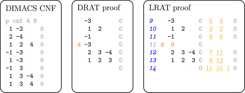 Figure 1
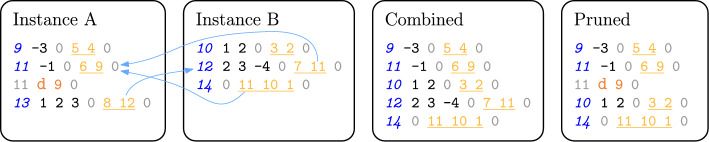 Figure 2
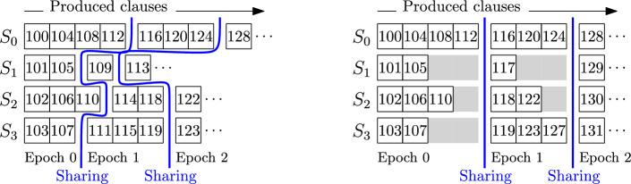 Figure 3
 Figure 4
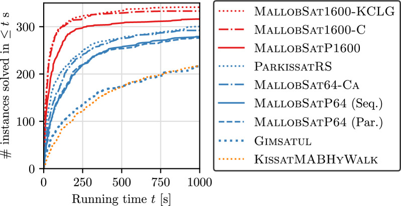 Figure 5
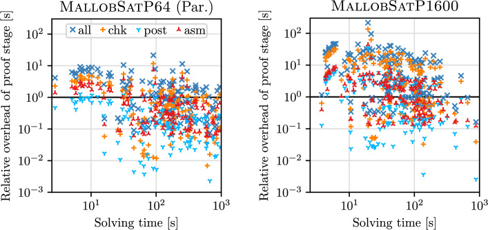 Figure 6
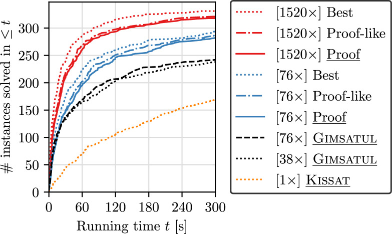 Figure 7
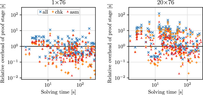 Figure 8
 Figure 9
- —http://dx.doi.org/10.13039/100010663H2020 European Research Council
- —National Science Foundation
- —Karlsruher Institut für Technologie (KIT) (4220)
Peer Reviews
No public reviews on file for this paper yet. If you reviewed it on a platform where reviews are public (OpenReview, ICLR, NeurIPS, ICML), you can paste yours below so the community can read it here.
Videos
No videos yet. Explain this paper in a talk, walkthrough, or lecture? Add one.
Taxonomy
TopicsFormal Methods in Verification · Logic, programming, and type systems · Model-Driven Software Engineering Techniques
Introduction
SAT solvers are general-purpose tools for solving complex computational problems. By encoding domain problems into propositional logic, users have successfully applied SAT solvers in a plethora of relevant fields such as formal verification [49], electronic design automation [33], and mathematics [12]. The list of applications has grown significantly over the years, mainly because algorithmic improvements have led to orders of magnitude improvement in the performance of the best sequential solvers [9].
Despite all this progress, there are still many problems that cannot be solved quickly with even the best sequential solvers, pushing researchers to explore ways of parallelizing SAT solving. One approach that has worked well for specific problem instances is Cube-and-Conquer [25, 28], which can achieve near-linear speedups for thousands of cores but requires domain knowledge about how effectively to split a problem into subproblems. An alternative approach that does not require such knowledge is clause-sharing portfolio solving [21], which has recently led to distributed solvers [44] achieving impressive speedups (e.g., 40–400 \documentclass[12pt]{minimal} \usepackage{amsmath} \usepackage{wasysym} \usepackage{amsfonts} \usepackage{amssymb} \usepackage{amsbsy} \usepackage{mathrsfs} \usepackage{upgreek} \setlength{\oddsidemargin}{-69pt} \begin{document}$$\times $$\end{document} at 3000 cores, depending on problem difficulty [45]) over the best sequential solvers across broad sets of benchmarks [19].
Today, distributed clause-sharing SAT solvers are some of the most powerful tools available for solving hard SAT problems. However, there is an important caveat: unlike sequential solvers, current distributed clause-sharing solvers cannot produce proofs of unsatisfiability. A direct consequence is that these distributed solvers cannot be used for proving theorems [23, 28, 46]. Even in cases where proofs are not strictly required, it is important to be able to trust the output of an algorithm.1 For instance, in bounded model checking [14]—a crucial verification tool and one of the most prominent applications of SAT solving—a formula’s reported unsatisfiability is interpreted as a system behaving correctly up to the considered bound. Therefore, the safety and reliability of crucial systems may depend on a SAT solver answering correctly.
In this sense, we argue that distributed clause-sharing solvers are lacking compared to sequential SAT solvers in terms of general trustworthiness. The latter, while complex pieces of software, not only generate verifiable proofs but are also being rigorously tested (e.g., [6, 13]) and feature limited external interfaces. Distributed clause-sharing solvers, on the other hand,
- are more costly (and thus more difficult) to test rigorously;
- make use of several different SAT solvers configured in many different ways [3];
- run many execution threads concurrently; and
- make use of non-trivial interfaces for data transfer such as message passing [3] and inter-process communication [44]. All of these properties have some potential to introduce faults or correctness issues in certain corner cases, which makes it all the more critical to be able to verify the system’s output independently.
Although there has been foundational work in producing proofs for shared-memory clause-sharing SAT solvers [7, 27], existing approaches are not general enough for large-scale distributed portfolio solvers. In this work, we address this issue and present the first scalable approach for generating proofs for such solvers. To construct proofs, we maintain provenance information about shared clauses in order to track how they are used in the global solving process, and we use the recently-developed LRAT proof format [16] to track dependencies among partial proofs produced by solver instances. By exploiting these dependencies, we are then able to reconstruct a single linear proof from all the partial proofs produced by the sequential solvers. We first outline a simple sequential algorithm for proof reconstruction before devising a parallel algorithm that we implement in a fully distributed way. Both algorithms produce independently-verifiable proofs in the LRAT format. We demonstrate our approaches using an LRAT-producing version of the sequential SAT solver CaDiCaL [8] to turn it into a clause-sharing solver, and then modify MallobSat to orchestrate a portfolio of such CaDiCaL instances while tracking the IDs of all shared clauses.
We evaluate our approaches from the perspective of efficiency, benchmarking the performance of our clause-sharing portfolio solver against the winners of the cloud, parallel, and sequential tracks from ISC 2022. Our approach introduces overhead in terms of solving, proof reconstruction, and proof checking. We examine this overhead in detail and show that our approach is still considerably faster than sequential approaches. We also demonstrate that our approach substantially outperforms prior work on proof production for clause-sharing portfolios [27].
Finally, we discuss the latest advances in this area. Most notably, our initial work served as a motivation for Pollitt et al. to implement a sequential solver with full, efficient LRAT support [37]. Integrating this solver and dropping the previously required pre- and postprocessing stages now results in even better scaling behavior.
Context The article at hand is a significantly extended version of our TACAS 2023 conference publication [35]. We integrated supplementary content from the corresponding author’s dissertation [42], notably a proof of correctness for our distributed proof production approach and a more detailed analysis of experiments. Furthermore, we describe important recent developments in this topic and are able to present significantly improved results in follow-up experiments. Since these latest results complement our original results, which feature a less developed setup but more competitors and analyses, we include both of them as important stages in our line of work.
This article is structured as follows. In Sect. 2, we provide the relevant background for our discussion. In Sect. 3, we outline the general problem of producing proofs for distributed SAT solving and a first sequential algorithm for proof combination. In Sect. 4, we describe a more general algorithm for distributed-memory setups. We discuss our original implementation in Sect. 5 and the according empirical evaluation in Sect. 6, then we describe and assess our latest advances on the topic in Sect. 7. We conclude with a summary and an outlook in Sect. 8.
Background
In this section, we introduce relevant preliminaries for the paper, including SAT, proofs of unsatisfiability, and parallel and distributed SAT solving.
The SAT Problem
A Boolean variable can only be true or false. A literal is a Boolean variable or its negation. A clause is a disjunction of literals, i.e., a logical expression that evaluates to true if and only if at least one of the literals in the clause is true. A Conjunctive Normal Form (CNF) formula is a conjunction of clauses, i.e., a logical expression that evaluates to true if and only if each of the clauses evaluates to true.
An assignment \documentclass[12pt]{minimal} \usepackage{amsmath} \usepackage{wasysym} \usepackage{amsfonts} \usepackage{amssymb} \usepackage{amsbsy} \usepackage{mathrsfs} \usepackage{upgreek} \setlength{\oddsidemargin}{-69pt} \begin{document}$$\alpha $$\end{document} for a logical expression F assigns values to some of the variables occurring in F. \documentclass[12pt]{minimal} \usepackage{amsmath} \usepackage{wasysym} \usepackage{amsfonts} \usepackage{amssymb} \usepackage{amsbsy} \usepackage{mathrsfs} \usepackage{upgreek} \setlength{\oddsidemargin}{-69pt} \begin{document}$$\alpha $$\end{document} is partial if some variables in F are left unassigned, and \documentclass[12pt]{minimal} \usepackage{amsmath} \usepackage{wasysym} \usepackage{amsfonts} \usepackage{amssymb} \usepackage{amsbsy} \usepackage{mathrsfs} \usepackage{upgreek} \setlength{\oddsidemargin}{-69pt} \begin{document}$$\alpha $$\end{document} is total otherwise. If \documentclass[12pt]{minimal} \usepackage{amsmath} \usepackage{wasysym} \usepackage{amsfonts} \usepackage{amssymb} \usepackage{amsbsy} \usepackage{mathrsfs} \usepackage{upgreek} \setlength{\oddsidemargin}{-69pt} \begin{document}$$\alpha $$\end{document} is total and F evaluates to true under \documentclass[12pt]{minimal} \usepackage{amsmath} \usepackage{wasysym} \usepackage{amsfonts} \usepackage{amssymb} \usepackage{amsbsy} \usepackage{mathrsfs} \usepackage{upgreek} \setlength{\oddsidemargin}{-69pt} \begin{document}$$\alpha $$\end{document} , then we write \documentclass[12pt]{minimal} \usepackage{amsmath} \usepackage{wasysym} \usepackage{amsfonts} \usepackage{amssymb} \usepackage{amsbsy} \usepackage{mathrsfs} \usepackage{upgreek} \setlength{\oddsidemargin}{-69pt} \begin{document}$$\alpha \models F$$\end{document} and say that \documentclass[12pt]{minimal} \usepackage{amsmath} \usepackage{wasysym} \usepackage{amsfonts} \usepackage{amssymb} \usepackage{amsbsy} \usepackage{mathrsfs} \usepackage{upgreek} \setlength{\oddsidemargin}{-69pt} \begin{document}$$\alpha $$\end{document} is a model for F or that \documentclass[12pt]{minimal} \usepackage{amsmath} \usepackage{wasysym} \usepackage{amsfonts} \usepackage{amssymb} \usepackage{amsbsy} \usepackage{mathrsfs} \usepackage{upgreek} \setlength{\oddsidemargin}{-69pt} \begin{document}$$\alpha $$\end{document} satisfies F. We refer to such an assignment as a satisfying assignment (for F). A CNF formula F is satisfiable if and only if a satisfying assignment to F exists. Otherwise, F is unsatisfiable.
An instance of the SAT decision problem is given as a CNF formula F. The task is to decide whether F is satisfiable. A common extension of the SAT decision problem, which we refer to as the constructive SAT problem, additionally requires outputting a satisfying assignment \documentclass[12pt]{minimal} \usepackage{amsmath} \usepackage{wasysym} \usepackage{amsfonts} \usepackage{amssymb} \usepackage{amsbsy} \usepackage{mathrsfs} \usepackage{upgreek} \setlength{\oddsidemargin}{-69pt} \begin{document}$$\alpha $$\end{document} if F was found to be satisfiable. Likewise, we consider the certified SAT problem as an extension of the constructive SAT problem which additionally requires outputting an unsatisfiability certificate \documentclass[12pt]{minimal} \usepackage{amsmath} \usepackage{wasysym} \usepackage{amsfonts} \usepackage{amssymb} \usepackage{amsbsy} \usepackage{mathrsfs} \usepackage{upgreek} \setlength{\oddsidemargin}{-69pt} \begin{document}$${\mathcal {C}}$$\end{document} if F was found to be unsatisfiable. Intuitively, an unsatisfiability certificate is a chain of logical reasoning that the solver used to derive unsatisfiability and that others can verify independently.
Today’s most efficient sequential SAT solvers commonly build upon the Conflict-Driven Clause Learning (CDCL) approach [34]. Intuitively, the solver carefully searches the space of partial variable assignments and derives conflict clauses from encountered logical conflicts. These clauses can be useful to prune the search for a satisfying assignment on the one hand and to derive the empty clause, demonstrating unsatisfiability, on the other hand. Maintaining and garbage-collecting learned clauses in a sensible manner is an important line of research in SAT solving [1, 36].
Proofs of Unsatisfiability
In contrast to the pure decision problem, the certified SAT problem requires a justification for the produced result. For the satisfiable case, this is straightforward. All common SAT solving approaches conclude the satisfiability of a formula by constructing a satisfying assignment. This assignment serves as a justification since it can be verified in linear time by evaluating the formula on the assignment. For the unsatisfiable case, the usual justification is the solver’s chain of logical reasoning leading to the empty clause, which demonstrates unsatisfiability. This chain is not necessarily linear in the problem input, and, in fact, certain inputs require an exponentially-sized proof when using common reasoning techniques [20, 24].
Consider a formula F and a sequence of clauses \documentclass[12pt]{minimal} \usepackage{amsmath} \usepackage{wasysym} \usepackage{amsfonts} \usepackage{amssymb} \usepackage{amsbsy} \usepackage{mathrsfs} \usepackage{upgreek} \setlength{\oddsidemargin}{-69pt} \begin{document}$$C := \langle c_1, c_2, \ldots , c_n \rangle $$\end{document} learned by a CDCL solver S while processing F. The last clause \documentclass[12pt]{minimal} \usepackage{amsmath} \usepackage{wasysym} \usepackage{amsfonts} \usepackage{amssymb} \usepackage{amsbsy} \usepackage{mathrsfs} \usepackage{upgreek} \setlength{\oddsidemargin}{-69pt} \begin{document}$$c_n$$\end{document} is the empty clause, i.e., the solver has derived unsatisfiability for F. In order to verify that the result is correct, we can check for each \documentclass[12pt]{minimal} \usepackage{amsmath} \usepackage{wasysym} \usepackage{amsfonts} \usepackage{amssymb} \usepackage{amsbsy} \usepackage{mathrsfs} \usepackage{upgreek} \setlength{\oddsidemargin}{-69pt} \begin{document}$$i \in \{1, \ldots , n\}$$\end{document} if \documentclass[12pt]{minimal} \usepackage{amsmath} \usepackage{wasysym} \usepackage{amsfonts} \usepackage{amssymb} \usepackage{amsbsy} \usepackage{mathrsfs} \usepackage{upgreek} \setlength{\oddsidemargin}{-69pt} \begin{document}$$c_i$$\end{document} is indeed a logical implication of the prior formula:
\documentclass[12pt]{minimal} \usepackage{amsmath} \usepackage{wasysym} \usepackage{amsfonts} \usepackage{amssymb} \usepackage{amsbsy} \usepackage{mathrsfs} \usepackage{upgreek} \setlength{\oddsidemargin}{-69pt} \begin{document}$$\begin{aligned} \left( F \cup \bigcup _{j=1}^{i-1} c_j\right) {\mathop {\Rightarrow }\limits ^{?}} c_i \end{aligned}$$\end{document}Many clause learning and preprocessing techniques have a convenient property named the Reverse Unit Propagation (RUP) property [48]. For any clause found with the RUP property, the check above can always be achieved by means of unit propagation: We assert each literal of \documentclass[12pt]{minimal} \usepackage{amsmath} \usepackage{wasysym} \usepackage{amsfonts} \usepackage{amssymb} \usepackage{amsbsy} \usepackage{mathrsfs} \usepackage{upgreek} \setlength{\oddsidemargin}{-69pt} \begin{document}$$c_i$$\end{document} to be false and then check if unit propagation leads to a direct conflict. In this case, we showed that \documentclass[12pt]{minimal} \usepackage{amsmath} \usepackage{wasysym} \usepackage{amsfonts} \usepackage{amssymb} \usepackage{amsbsy} \usepackage{mathrsfs} \usepackage{upgreek} \setlength{\oddsidemargin}{-69pt} \begin{document}$$F \wedge \lnot c_i$$\end{document} is unsatisfiable, hence \documentclass[12pt]{minimal} \usepackage{amsmath} \usepackage{wasysym} \usepackage{amsfonts} \usepackage{amssymb} \usepackage{amsbsy} \usepackage{mathrsfs} \usepackage{upgreek} \setlength{\oddsidemargin}{-69pt} \begin{document}$$c_i$$\end{document} is a logical consequence of F and S was correct to derive it. If no conflict arises from unit propagation, \documentclass[12pt]{minimal} \usepackage{amsmath} \usepackage{wasysym} \usepackage{amsfonts} \usepackage{amssymb} \usepackage{amsbsy} \usepackage{mathrsfs} \usepackage{upgreek} \setlength{\oddsidemargin}{-69pt} \begin{document}$$c_i$$\end{document} is not a sound RUP clause and we reject the proof. Performing this check for the entire sequence C is a means of verifying the result of S.
Propagating each clause in C through F can be expensive, and for large derivations we cannot keep the entirety of \documentclass[12pt]{minimal} \usepackage{amsmath} \usepackage{wasysym} \usepackage{amsfonts} \usepackage{amssymb} \usepackage{amsbsy} \usepackage{mathrsfs} \usepackage{upgreek} \setlength{\oddsidemargin}{-69pt} \begin{document}$$F \cup C$$\end{document} in memory. Therefore, a popular extension of proof formats allows the deletion of clauses [22]. Whenever S deletes a clause, it logs this deletion just like it logs learned clauses. This deletion can then be mirrored by the proof checker traversing the proof. A proof certificate now takes the shape \documentclass[12pt]{minimal} \usepackage{amsmath} \usepackage{wasysym} \usepackage{amsfonts} \usepackage{amssymb} \usepackage{amsbsy} \usepackage{mathrsfs} \usepackage{upgreek} \setlength{\oddsidemargin}{-69pt} \begin{document}$${\mathcal {C}} := \langle a_1, a_2, \ldots , a_{n'} \rangle $$\end{document} where \documentclass[12pt]{minimal} \usepackage{amsmath} \usepackage{wasysym} \usepackage{amsfonts} \usepackage{amssymb} \usepackage{amsbsy} \usepackage{mathrsfs} \usepackage{upgreek} \setlength{\oddsidemargin}{-69pt} \begin{document}$$a_i = (\textit{op}, c_i)$$\end{document} , \documentclass[12pt]{minimal} \usepackage{amsmath} \usepackage{wasysym} \usepackage{amsfonts} \usepackage{amssymb} \usepackage{amsbsy} \usepackage{mathrsfs} \usepackage{upgreek} \setlength{\oddsidemargin}{-69pt} \begin{document}$$\textit{op} \in \{\textit{add}, \textit{delete}\}$$\end{document} , and \documentclass[12pt]{minimal} \usepackage{amsmath} \usepackage{wasysym} \usepackage{amsfonts} \usepackage{amssymb} \usepackage{amsbsy} \usepackage{mathrsfs} \usepackage{upgreek} \setlength{\oddsidemargin}{-69pt} \begin{document}$$c_i$$\end{document} is a clause.
The current standard format for proofs of unsatisfiability in sequential SAT solving is called DRAT [22], which allows for additions and deletions as outlined above. Each added clause must adhere to the so-called RAT criterion [22], a generalization of RUP that we do not detail. The more recent LRAT proof format [16] augments each clause addition with hints, or dependencies, that identify the clauses that were required to derive the current clause. This makes proof checking more efficient, and in fact the usual pipeline for trusted proof checking is first to use a fast unverified tool (e.g., [22]) to transform a DRAT proof into an LRAT proof, and then check the resulting LRAT proof with a formally verified proof checker [16, 29, 31, 47].Fig. 1CNF formula and corresponding DRAT and LRAT proofs of its unsatisfiability. Headers and separators are set in light gray, deletions begin with “d”, leading clause IDs are italicized, and hints are underlined. Clause literals are always colored black
Figure 1 shows a formula (left) and its corresponding DRAT proof (center) and LRAT proof (right). Each proof line in the LRAT proof starts with a clause ID. The numbering starts with ID 9 because the eight clauses of the original formula are assigned the IDs 1 to 8. Each clause addition first lists the literals of the clause and then the clause’s dependencies in the form of clause IDs. Clause deletions only state the ID(s) of the clauses to delete, as in the later deletion of clause |9|. In our work, we exploit the hints of LRAT to determine dependencies among distributed solvers.
Parallel and Distributed SAT Solving
The most common way to parallelize general-purpose SAT solving is to run a portfolio of sequential (mostly CDCL) solvers in parallel and to consider a problem solved as soon as one of the solvers finishes (c.f. [2–4, 17, 21, 32]). Given that the solvers are sufficiently diverse, portfolio solving is effective if all of the sequential solvers work independently but not efficient since only a single thread contributes to the final result. Scalability can be boosted significantly by having the solvers share information in the form of learned clauses [21]. This approach is taken by the distributed solver MallobSat [44, 45], which has dominated the cloud track of the International SAT competition since 2020 [15, 19, 41]. MallobSat relies on a communication-efficient aggregation strategy to collect the globally most useful distinct learned clauses and reliably to filter duplicates as well as previously-shared clauses [44]. This strategy aims to maximize the density and utility of the communicated data. As a matter of fact, MallobSat’s clause sharing was recently shown to be the main driver of its scalability, even if diversification is reduced to an absolute minimum, prompting its authors to use the term clause-sharing solver going forward [45].
Producing proofs of unsatisfiability is trivial for pure portfolio solvers if each of the employed solvers is able to output a proof itself. For clause-sharing portfolios, on the other hand, the derivation of the empty clause can depend on a clause produced by another solver, which may again depend on clauses from other solvers, and so on. The full chain of reasoning for a formula’s unsatisfiability can thus be a dense and interleaved network that features conflict clauses from all participating solvers.
Prior work on generating proofs from clause-sharing portfolio solvers is limited to shared-memory parallelism and cannot be generalized to distributed memory in any obvious manner. The recent shared-memory solver Gimsatul [7] is designed specifically to support outputting DRAT proofs; however, sequential checking of these proofs is “most likely is too slow to be run in practice” [7] and we are not aware of any notable parallel DRAT (or LRAT) checking approaches. In terms of generic clause-sharing portfolios, Heule et al. [27] attempted to generate proofs by having the solver threads emit proof lines concurrently into a single proof. Clause deletion statements can be added to the proof only after all solvers have reported deletion of the clause. Heule et al. obtained mixed results and for the most part were not able to arrive at proofs that are feasible to check, mostly due to the sheer size of the output and the large number of clauses that the checker is required to keep in memory.
Basic Proof Production
Our goal is to produce checkable unsatisfiability proofs for problems solved by distributed clause-sharing SAT solvers. We propose to reuse the work done on proofs for sequential solvers by having each solver produce a partial proof containing the clauses it learned. These partial proofs are invalid in general because each sequential solver can rely on clauses shared by other solvers when learning new clauses. For example, when solver A derives a new clause, it might rely on clauses from solvers B and C, which in turn relied on clauses from solvers D and E, and so on. The justification of A’s clause derivation is thus spread across multiple partial proofs. We need to combine the partial proofs into a single valid proof in which the clauses are in dependency order, meaning that each clause can be derived from previous clauses.
In order to produce efficiently checkable proofs in a scalable manner, we address the following three challenges:
- Provide metadata to identify which solver produced each learned clause.
- Efficiently sort learned clauses in dependency order across all solvers.
- Reduce proof sizes by removing unnecessary clauses. Switching from DRAT to the LRAT proof format provides the mechanism to unlock all three challenges. First, we specialize the clause-numbering scheme used by LRAT in order to distinguish the clauses produced by each solver. Second, we use the dependency information from LRAT to construct a complete proof from the partial proofs produced by each solver. Finally, we determine which clauses are unnecessary (or used only for parts of the proof) to trim the proof where possible.
Partial Proof Production
To combine the partial proofs into a complete proof, we modify the mechanism used to produce LRAT proofs in each of the individual sequential solvers. We assign to each clause an ID that is unique across solvers and identifies which solver originally derived it. The following mapping from clauses to IDs achieves uniqueness across solvers:
Definition 1
Let o be the number of clauses in the original formula and let p be the number of sequential solvers. Then the ID of the k-th derived clause ( \documentclass[12pt]{minimal} \usepackage{amsmath} \usepackage{wasysym} \usepackage{amsfonts} \usepackage{amssymb} \usepackage{amsbsy} \usepackage{mathrsfs} \usepackage{upgreek} \setlength{\oddsidemargin}{-69pt} \begin{document}$$k \ge 0$$\end{document} ) of solver i is defined as \documentclass[12pt]{minimal} \usepackage{amsmath} \usepackage{wasysym} \usepackage{amsfonts} \usepackage{amssymb} \usepackage{amsbsy} \usepackage{mathrsfs} \usepackage{upgreek} \setlength{\oddsidemargin}{-69pt} \begin{document}$$\textit{ID}^{i}_{k} = o + i + pk$$\end{document} .
Given \documentclass[12pt]{minimal} \usepackage{amsmath} \usepackage{wasysym} \usepackage{amsfonts} \usepackage{amssymb} \usepackage{amsbsy} \usepackage{mathrsfs} \usepackage{upgreek} \setlength{\oddsidemargin}{-69pt} \begin{document}$$\textit{ID}^{i}_{k}$$\end{document} , we can easily determine the producing solver i using modular arithmetic.
We extend our clause sharing to send each clause together with its ID. A receiving solver stores the clause with its ID and uses the ID in proof hints when the clause is used locally, as it does with locally-derived clauses. Unlike locally-derived clauses, we add no derivation lines for incoming clauses to the local proof. Instead, these derivations will be added to the final proof when combining the partial proofs.
Partial Proof Combination
Once the distributed solver reports unsatisfiability, we have p partial proofs. The derivations in these proofs can refer to clauses of other partial proofs, but they are locally in dependency order. We can thus combine the partial proofs without reordering their clauses beforehand. We can simply interleave their clauses so the resulting proof is also in dependency order, ignoring any deletions in the partial proofs.
Our combination algorithm traverses the partial proofs round-robin. At each step, we read and output the next clause c from the current partial proof as long as all dependencies of c have already been output. Checking whether a dependency d has already been output is simple: We determine which solver produced d (see Definition 1) and check if the next clause of the corresponding partial proof has an ID higher than d. Our algorithm terminates when it emits the empty clause.Fig. 2. Partial proofs and combined and pruned proof, colored as in Fig. 1. Arrows indicate remote dependencies across the partial proofs
Suppose that two clause-sharing solver instances, A and B, found the formula from Fig. 1 to be unsatisfiable and emitted two partial proofs as shown in Fig. 2. Starting with A, we can emit clause 9 (only depending on original clauses) and 11 (depending on original clauses and clause 9). We cannot emit clause 13 since it depends on clause 12 from B. Proceeding with B, we can now emit the remaining clauses 10, 12, and 14. Since clause 14 is the empty clause, we finish with the complete proof shown in Fig. 2 (middle right). Note that clause 13 was not added to the combined proof as it was not required to satisfy any dependencies of the empty clause.
Proof Pruning
The combined proof our procedure produces is valid but not efficiently checkable because (1) it can contain superfluous clauses and (2) it does not contain deletion lines, meaning that a proof checker must maintain all learned clauses in memory throughout the checking process. To reduce size and improve checking performance, we prune our combined proof to contain only necessary clauses, and we add deletion statements for clauses as soon as they are not needed anymore.
Our pruning algorithm walks the combined proof in reverse to find all transitive dependencies of the empty clause, similar to backward checking of DRAT proofs [26]. We maintain a set R of clause IDs required in the proof, initialized to the ID of the empty clause alone. We then read all clauses in reverse order, including the empty clause. Clauses that are not required are ignored. When encountering a clause derivation whose ID is in R, we check for each of its dependencies whether this is the first time (from the proof’s end) we see this dependency. In such cases, we can emit a deletion line for the dependency since it is the last time the clause is used in the proof. After checking all its dependencies, we output the required clause derivation and add its dependencies (except for original clauses) to R. The final output of the algorithm is a proof in reversed order, where each clause is required for some derivation and deleted as soon as it is no longer required. Reversing this output line by line yields a sound and compact proof.
Consider the combined proof in Fig. 2. Working backward from clause 14, with clause IDs 11 and 10 added to R, we determine that clause 12 is not required, so it is ignored. Additionally, prior to clause 11, clause 9 is not in R, so it can be deleted after the derivation of clause 11. As such, we arrive at the pruned proof in Fig. 2.
On realistic proofs, we show in Sect. 6 that pruning can sometimes reduce the proof size by several orders of magnitude.
Distributed Proof Production
The proof production as described above is sequential and may process huge amounts of data, all of which needs to be accessible from the machine that executes the procedure. In addition, maintaining the required clause IDs during the procedure can require a prohibitive amount of memory for large proofs. In the following, we propose an efficient distributed approach to proof production that addresses these scalability issues by exploiting some key properties of periodic all-to-all clause sharing.
Overview
Our sequential algorithm first combines all partial proofs into a single proof and then prunes unneeded proof lines. In contrast, our distributed algorithm first prunes all partial proofs in parallel and only then merges the required lines into one file.
As our distributed execution environment, let us assume a two-level hierarchy where we have m processes which run \documentclass[12pt]{minimal} \usepackage{amsmath} \usepackage{wasysym} \usepackage{amsfonts} \usepackage{amssymb} \usepackage{amsbsy} \usepackage{mathrsfs} \usepackage{upgreek} \setlength{\oddsidemargin}{-69pt} \begin{document}$$c \ge 1$$\end{document} solver threads each, amounting to a total of \documentclass[12pt]{minimal} \usepackage{amsmath} \usepackage{wasysym} \usepackage{amsfonts} \usepackage{amssymb} \usepackage{amsbsy} \usepackage{mathrsfs} \usepackage{upgreek} \setlength{\oddsidemargin}{-69pt} \begin{document}$$p = mc$$\end{document} solvers. Furthermore, we assume that clauses are shared in an all-to-all fashion (i.e., every solver may receive clauses from every other solver) in periodic intervals. Both of these assumptions hold for the popular distributed systems HordeSat [3] and MallobSat [44]. We refer to the intervals between subsequent sharing operations as epochs. Consider Fig. 3 (left): Clause 118 was produced by \documentclass[12pt]{minimal} \usepackage{amsmath} \usepackage{wasysym} \usepackage{amsfonts} \usepackage{amssymb} \usepackage{amsbsy} \usepackage{mathrsfs} \usepackage{upgreek} \setlength{\oddsidemargin}{-69pt} \begin{document}$$S_2$$\end{document} in epoch 1. Its derivation may depend on local clause 114 and on any of the 11 clauses produced in epoch 0, but it cannot depend on, e.g., clause 109 or 111 since these clauses have been produced after the last clause sharing. More generally, a clause c produced by solver i during epoch e can only depend on (1) earlier clauses by solver i produced during epoch e or earlier, and (2) clauses by solvers \documentclass[12pt]{minimal} \usepackage{amsmath} \usepackage{wasysym} \usepackage{amsfonts} \usepackage{amssymb} \usepackage{amsbsy} \usepackage{mathrsfs} \usepackage{upgreek} \setlength{\oddsidemargin}{-69pt} \begin{document}$$j \ne i$$\end{document} produced before epoch e.
Using this knowledge, we can rewind the solving procedure. Each process reads its partial proofs in reverse, outputs each line that adds a required clause, and adds the line’s dependencies to the required clauses. Required remote clauses produced in epoch e are transferred to their origin before any process begins to read proof lines from epoch e. As such, whenever a process reads a proof line, it knows if the clause is required. We later explain how the outputs of all processes can be merged.Fig. 3. Four solvers work on a formula with 99 original clauses, produce new clauses (depicted by their ID) and share clauses periodically, without (left) and with (right) clause ID alignment
Clause ID Alignment
To synchronize the reading and redistribution of clause IDs in our distributed pruning, we need a way to decide from which epoch a remote clause ID originates. However, solvers generally produce clauses with different speeds, so the IDs by different solvers will likely be in dissimilar ranges within the same epoch over time. For instance, in Fig. 3 (left) solver \documentclass[12pt]{minimal} \usepackage{amsmath} \usepackage{wasysym} \usepackage{amsfonts} \usepackage{amssymb} \usepackage{amsbsy} \usepackage{mathrsfs} \usepackage{upgreek} \setlength{\oddsidemargin}{-69pt} \begin{document}$$S_3$$\end{document} has no way of knowing from which epoch clause 118 originates. To solve this issue, we propose to align all produced clause IDs after each sharing. During solving, we add a certain offset \documentclass[12pt]{minimal} \usepackage{amsmath} \usepackage{wasysym} \usepackage{amsfonts} \usepackage{amssymb} \usepackage{amsbsy} \usepackage{mathrsfs} \usepackage{upgreek} \setlength{\oddsidemargin}{-69pt} \begin{document}$$\delta _i^e$$\end{document} to each ID produced by solver i in epoch e. As such, we can associate each epoch e with a global interval \documentclass[12pt]{minimal} \usepackage{amsmath} \usepackage{wasysym} \usepackage{amsfonts} \usepackage{amssymb} \usepackage{amsbsy} \usepackage{mathrsfs} \usepackage{upgreek} \setlength{\oddsidemargin}{-69pt} \begin{document}$$[ A_e, A_{e+1} )$$\end{document} that contains all clause IDs produced in that epoch. In Fig. 3 (right), \documentclass[12pt]{minimal} \usepackage{amsmath} \usepackage{wasysym} \usepackage{amsfonts} \usepackage{amssymb} \usepackage{amsbsy} \usepackage{mathrsfs} \usepackage{upgreek} \setlength{\oddsidemargin}{-69pt} \begin{document}$$A_0 = 0$$\end{document} , \documentclass[12pt]{minimal} \usepackage{amsmath} \usepackage{wasysym} \usepackage{amsfonts} \usepackage{amssymb} \usepackage{amsbsy} \usepackage{mathrsfs} \usepackage{upgreek} \setlength{\oddsidemargin}{-69pt} \begin{document}$$A_1 = 116$$\end{document} , and \documentclass[12pt]{minimal} \usepackage{amsmath} \usepackage{wasysym} \usepackage{amsfonts} \usepackage{amssymb} \usepackage{amsbsy} \usepackage{mathrsfs} \usepackage{upgreek} \setlength{\oddsidemargin}{-69pt} \begin{document}$$A_2 = 128$$\end{document} . Clause 118 on the left has been aligned to 122 on the right ( \documentclass[12pt]{minimal} \usepackage{amsmath} \usepackage{wasysym} \usepackage{amsfonts} \usepackage{amssymb} \usepackage{amsbsy} \usepackage{mathrsfs} \usepackage{upgreek} \setlength{\oddsidemargin}{-69pt} \begin{document}$$\delta _2^1 = 4$$\end{document} ) and due to \documentclass[12pt]{minimal} \usepackage{amsmath} \usepackage{wasysym} \usepackage{amsfonts} \usepackage{amssymb} \usepackage{amsbsy} \usepackage{mathrsfs} \usepackage{upgreek} \setlength{\oddsidemargin}{-69pt} \begin{document}$$A_1 \le 122 < A_2$$\end{document} all solvers know that this clause originates from epoch 1.
Initially, \documentclass[12pt]{minimal} \usepackage{amsmath} \usepackage{wasysym} \usepackage{amsfonts} \usepackage{amssymb} \usepackage{amsbsy} \usepackage{mathrsfs} \usepackage{upgreek} \setlength{\oddsidemargin}{-69pt} \begin{document}$$\delta _i^0 := 0$$\end{document} for all i. Let \documentclass[12pt]{minimal} \usepackage{amsmath} \usepackage{wasysym} \usepackage{amsfonts} \usepackage{amssymb} \usepackage{amsbsy} \usepackage{mathrsfs} \usepackage{upgreek} \setlength{\oddsidemargin}{-69pt} \begin{document}$$I_i^e$$\end{document} be the first original (unaligned) ID produced by solver i in epoch e. With the sharing that initiates epoch \documentclass[12pt]{minimal} \usepackage{amsmath} \usepackage{wasysym} \usepackage{amsfonts} \usepackage{amssymb} \usepackage{amsbsy} \usepackage{mathrsfs} \usepackage{upgreek} \setlength{\oddsidemargin}{-69pt} \begin{document}$$e>0$$\end{document} , we want to define the common start of epoch e, \documentclass[12pt]{minimal} \usepackage{amsmath} \usepackage{wasysym} \usepackage{amsfonts} \usepackage{amssymb} \usepackage{amsbsy} \usepackage{mathrsfs} \usepackage{upgreek} \setlength{\oddsidemargin}{-69pt} \begin{document}$$A_e$$\end{document} , to be larger than all aligned clause IDs from epoch \documentclass[12pt]{minimal} \usepackage{amsmath} \usepackage{wasysym} \usepackage{amsfonts} \usepackage{amssymb} \usepackage{amsbsy} \usepackage{mathrsfs} \usepackage{upgreek} \setlength{\oddsidemargin}{-69pt} \begin{document}$$e-1$$\end{document} but no larger than any aligned clause ID from epoch e. We align each solver’s first ID from epoch e via the prior offset: \documentclass[12pt]{minimal} \usepackage{amsmath} \usepackage{wasysym} \usepackage{amsfonts} \usepackage{amssymb} \usepackage{amsbsy} \usepackage{mathrsfs} \usepackage{upgreek} \setlength{\oddsidemargin}{-69pt} \begin{document}$$I_{i}^e + \delta _{i}^{e-1}$$\end{document} . We then normalize each such ID by subtracting the solver’s individual offset i. Since two subsequent unaligned clause IDs always differ by p (the total number of solvers) and since \documentclass[12pt]{minimal} \usepackage{amsmath} \usepackage{wasysym} \usepackage{amsfonts} \usepackage{amssymb} \usepackage{amsbsy} \usepackage{mathrsfs} \usepackage{upgreek} \setlength{\oddsidemargin}{-69pt} \begin{document}$$i<p$$\end{document} , we know that \documentclass[12pt]{minimal} \usepackage{amsmath} \usepackage{wasysym} \usepackage{amsfonts} \usepackage{amssymb} \usepackage{amsbsy} \usepackage{mathrsfs} \usepackage{upgreek} \setlength{\oddsidemargin}{-69pt} \begin{document}$$I_{i}^e + \delta _{i}^{e-1} - i$$\end{document} is larger than the last ID solver i produced in epoch \documentclass[12pt]{minimal} \usepackage{amsmath} \usepackage{wasysym} \usepackage{amsfonts} \usepackage{amssymb} \usepackage{amsbsy} \usepackage{mathrsfs} \usepackage{upgreek} \setlength{\oddsidemargin}{-69pt} \begin{document}$$e-1$$\end{document} . We thus compute \documentclass[12pt]{minimal} \usepackage{amsmath} \usepackage{wasysym} \usepackage{amsfonts} \usepackage{amssymb} \usepackage{amsbsy} \usepackage{mathrsfs} \usepackage{upgreek} \setlength{\oddsidemargin}{-69pt} \begin{document}$$A_e$$\end{document} as the maximum of these values: \documentclass[12pt]{minimal} \usepackage{amsmath} \usepackage{wasysym} \usepackage{amsfonts} \usepackage{amssymb} \usepackage{amsbsy} \usepackage{mathrsfs} \usepackage{upgreek} \setlength{\oddsidemargin}{-69pt} \begin{document}$$A_e := \max _{i}\{ I_{i}^e + \delta _{i}^{e-1} - i\}$$\end{document} . Next, we want to compute new offsets \documentclass[12pt]{minimal} \usepackage{amsmath} \usepackage{wasysym} \usepackage{amsfonts} \usepackage{amssymb} \usepackage{amsbsy} \usepackage{mathrsfs} \usepackage{upgreek} \setlength{\oddsidemargin}{-69pt} \begin{document}$$\delta _i^e$$\end{document} in such a way that the first aligned clause ID of solver i in epoch e, \documentclass[12pt]{minimal} \usepackage{amsmath} \usepackage{wasysym} \usepackage{amsfonts} \usepackage{amssymb} \usepackage{amsbsy} \usepackage{mathrsfs} \usepackage{upgreek} \setlength{\oddsidemargin}{-69pt} \begin{document}$$I_i^e + \delta _i^e$$\end{document} , is equal to \documentclass[12pt]{minimal} \usepackage{amsmath} \usepackage{wasysym} \usepackage{amsfonts} \usepackage{amssymb} \usepackage{amsbsy} \usepackage{mathrsfs} \usepackage{upgreek} \setlength{\oddsidemargin}{-69pt} \begin{document}$$A_e + i$$\end{document} . Consequently, we set \documentclass[12pt]{minimal} \usepackage{amsmath} \usepackage{wasysym} \usepackage{amsfonts} \usepackage{amssymb} \usepackage{amsbsy} \usepackage{mathrsfs} \usepackage{upgreek} \setlength{\oddsidemargin}{-69pt} \begin{document}$$\delta _i^e := A_e + i - I_i^e$$\end{document} .
If we export a clause produced in epoch e by solver i, we add \documentclass[12pt]{minimal} \usepackage{amsmath} \usepackage{wasysym} \usepackage{amsfonts} \usepackage{amssymb} \usepackage{amsbsy} \usepackage{mathrsfs} \usepackage{upgreek} \setlength{\oddsidemargin}{-69pt} \begin{document}$$\delta _i^e$$\end{document} to its ID, and if we import shared clauses to i, we filter any clauses produced by i itself. Note that we do not modify the solvers’ internal ID counters nor the proofs they output, and there is no need to block or synchronize the solver threads at any time. Later, when reading the partial proof of solver i at epoch e, we need to add \documentclass[12pt]{minimal} \usepackage{amsmath} \usepackage{wasysym} \usepackage{amsfonts} \usepackage{amssymb} \usepackage{amsbsy} \usepackage{mathrsfs} \usepackage{upgreek} \setlength{\oddsidemargin}{-69pt} \begin{document}$$\delta _i^e$$\end{document} to each ID originating from solver i. All remote clause IDs in the partial proofs are already aligned.
Rewind Algorithm
Assume that solver \documentclass[12pt]{minimal} \usepackage{amsmath} \usepackage{wasysym} \usepackage{amsfonts} \usepackage{amssymb} \usepackage{amsbsy} \usepackage{mathrsfs} \usepackage{upgreek} \setlength{\oddsidemargin}{-69pt} \begin{document}$$u \in \{1,\ldots ,p\}$$\end{document} has derived the empty clause in epoch \documentclass[12pt]{minimal} \usepackage{amsmath} \usepackage{wasysym} \usepackage{amsfonts} \usepackage{amssymb} \usepackage{amsbsy} \usepackage{mathrsfs} \usepackage{upgreek} \setlength{\oddsidemargin}{-69pt} \begin{document}$${\hat{e}}$$\end{document} . Each process has a frontier \documentclass[12pt]{minimal} \usepackage{amsmath} \usepackage{wasysym} \usepackage{amsfonts} \usepackage{amssymb} \usepackage{amsbsy} \usepackage{mathrsfs} \usepackage{upgreek} \setlength{\oddsidemargin}{-69pt} \begin{document}$$R_i$$\end{document} for each process-local solver i. Each \documentclass[12pt]{minimal} \usepackage{amsmath} \usepackage{wasysym} \usepackage{amsfonts} \usepackage{amssymb} \usepackage{amsbsy} \usepackage{mathrsfs} \usepackage{upgreek} \setlength{\oddsidemargin}{-69pt} \begin{document}$$R_i$$\end{document} features the required clauses produced by i. In addition, each process has a backlog B of remote required clauses. B and \documentclass[12pt]{minimal} \usepackage{amsmath} \usepackage{wasysym} \usepackage{amsfonts} \usepackage{amssymb} \usepackage{amsbsy} \usepackage{mathrsfs} \usepackage{upgreek} \setlength{\oddsidemargin}{-69pt} \begin{document}$$R_i$$\end{document} are maximum-first priority queues of clause IDs. Initially, \documentclass[12pt]{minimal} \usepackage{amsmath} \usepackage{wasysym} \usepackage{amsfonts} \usepackage{amssymb} \usepackage{amsbsy} \usepackage{mathrsfs} \usepackage{upgreek} \setlength{\oddsidemargin}{-69pt} \begin{document}$$R_u$$\end{document} contains the ID of the empty clause while all other frontiers and backlogs are empty. Iteration \documentclass[12pt]{minimal} \usepackage{amsmath} \usepackage{wasysym} \usepackage{amsfonts} \usepackage{amssymb} \usepackage{amsbsy} \usepackage{mathrsfs} \usepackage{upgreek} \setlength{\oddsidemargin}{-69pt} \begin{document}$$x \ge 0$$\end{document} of our algorithm processes epoch \documentclass[12pt]{minimal} \usepackage{amsmath} \usepackage{wasysym} \usepackage{amsfonts} \usepackage{amssymb} \usepackage{amsbsy} \usepackage{mathrsfs} \usepackage{upgreek} \setlength{\oddsidemargin}{-69pt} \begin{document}$${\hat{e}}-x$$\end{document} and features two stages:
- Processing: Each process continues to read its partial proofs in reverse order from the final derived clause of the current epoch. If a line from solver i is read whose clause ID is at the top of \documentclass[12pt]{minimal} \usepackage{amsmath} \usepackage{wasysym} \usepackage{amsfonts} \usepackage{amssymb} \usepackage{amsbsy} \usepackage{mathrsfs} \usepackage{upgreek} \setlength{\oddsidemargin}{-69pt} \begin{document}$$R_i$$\end{document} , then the ID is removed from \documentclass[12pt]{minimal} \usepackage{amsmath} \usepackage{wasysym} \usepackage{amsfonts} \usepackage{amssymb} \usepackage{amsbsy} \usepackage{mathrsfs} \usepackage{upgreek} \setlength{\oddsidemargin}{-69pt} \begin{document}$$R_i$$\end{document} , the line is output, and each clause ID hint h in the line is treated as follows:
- h is inserted in \documentclass[12pt]{minimal} \usepackage{amsmath} \usepackage{wasysym} \usepackage{amsfonts} \usepackage{amssymb} \usepackage{amsbsy} \usepackage{mathrsfs} \usepackage{upgreek} \setlength{\oddsidemargin}{-69pt} \begin{document}$$R_{j}$$\end{document} if local solver j (possibly \documentclass[12pt]{minimal} \usepackage{amsmath} \usepackage{wasysym} \usepackage{amsfonts} \usepackage{amssymb} \usepackage{amsbsy} \usepackage{mathrsfs} \usepackage{upgreek} \setlength{\oddsidemargin}{-69pt} \begin{document}$$j=i$$\end{document} ) produced h.
- h is inserted in B if a remote solver produced h.
- h is ignored if h is an ID of an original clause of the problem. Reading stops as soon as a line’s ID precedes epoch \documentclass[12pt]{minimal} \usepackage{amsmath} \usepackage{wasysym} \usepackage{amsfonts} \usepackage{amssymb} \usepackage{amsbsy} \usepackage{mathrsfs} \usepackage{upgreek} \setlength{\oddsidemargin}{-69pt} \begin{document}$$e = {\hat{e}}-x$$\end{document} . Each \documentclass[12pt]{minimal} \usepackage{amsmath} \usepackage{wasysym} \usepackage{amsfonts} \usepackage{amssymb} \usepackage{amsbsy} \usepackage{mathrsfs} \usepackage{upgreek} \setlength{\oddsidemargin}{-69pt} \begin{document}$$R_i$$\end{document} as well as B now only contain clauses produced before e.
- Task redistribution: Each process extracts all clause IDs from B that were produced during \documentclass[12pt]{minimal} \usepackage{amsmath} \usepackage{wasysym} \usepackage{amsfonts} \usepackage{amssymb} \usepackage{amsbsy} \usepackage{mathrsfs} \usepackage{upgreek} \setlength{\oddsidemargin}{-69pt} \begin{document}$${\hat{e}}-x-1$$\end{document} . These clause IDs are aggregated among all processes. In our concrete implementation, we reuse MallobSat’s compact clause exchange operation [45], adjusted to aggregate clause IDs instead of clauses. This also allows us to eliminate duplicates among the redistributed IDs. Each process then traverses the aggregated clause IDs, and each clause produced by a local solver i is added to \documentclass[12pt]{minimal} \usepackage{amsmath} \usepackage{wasysym} \usepackage{amsfonts} \usepackage{amssymb} \usepackage{amsbsy} \usepackage{mathrsfs} \usepackage{upgreek} \setlength{\oddsidemargin}{-69pt} \begin{document}$$R_i$$\end{document} . Our algorithm stops in iteration \documentclass[12pt]{minimal} \usepackage{amsmath} \usepackage{wasysym} \usepackage{amsfonts} \usepackage{amssymb} \usepackage{amsbsy} \usepackage{mathrsfs} \usepackage{upgreek} \setlength{\oddsidemargin}{-69pt} \begin{document}$${\hat{e}}$$\end{document} after the processing stage, at which point all frontiers and backlogs are empty and all relevant proof lines have been output. The result is one partial proof per solver, with each partial proof containing the lines output by the corresponding solver.
Correctness
We now establish the correctness of our proof production. First, we show that our clause ID alignment works as intended:
Lemma 1
The alignment of clause IDs as described above results in a sequence \documentclass[12pt]{minimal} \usepackage{amsmath} \usepackage{wasysym} \usepackage{amsfonts} \usepackage{amssymb} \usepackage{amsbsy} \usepackage{mathrsfs} \usepackage{upgreek} \setlength{\oddsidemargin}{-69pt} \begin{document}$$A_0, A_1, A_2, \ldots , A_{{\hat{e}}}$$\end{document} such that for any clause with unaligned ID j produced by the i-th solver, \documentclass[12pt]{minimal} \usepackage{amsmath} \usepackage{wasysym} \usepackage{amsfonts} \usepackage{amssymb} \usepackage{amsbsy} \usepackage{mathrsfs} \usepackage{upgreek} \setlength{\oddsidemargin}{-69pt} \begin{document}$$A_e \le j+\delta _i^e < A_{e+1}$$\end{document} holds if and only if j was produced in epoch e.
Proof
We perform induction over epoch e in which a clause was produced.
For \documentclass[12pt]{minimal} \usepackage{amsmath} \usepackage{wasysym} \usepackage{amsfonts} \usepackage{amssymb} \usepackage{amsbsy} \usepackage{mathrsfs} \usepackage{upgreek} \setlength{\oddsidemargin}{-69pt} \begin{document}$$e=0$$\end{document} , we set \documentclass[12pt]{minimal} \usepackage{amsmath} \usepackage{wasysym} \usepackage{amsfonts} \usepackage{amssymb} \usepackage{amsbsy} \usepackage{mathrsfs} \usepackage{upgreek} \setlength{\oddsidemargin}{-69pt} \begin{document}$$A_0 = 0$$\end{document} . The first sharing defines \documentclass[12pt]{minimal} \usepackage{amsmath} \usepackage{wasysym} \usepackage{amsfonts} \usepackage{amssymb} \usepackage{amsbsy} \usepackage{mathrsfs} \usepackage{upgreek} \setlength{\oddsidemargin}{-69pt} \begin{document}$$A_1 = \max _{i}\{ I_{i}^1 + \delta _{i}^{0} - i\} = \max _{i}\{ I_{i}^1 - i\}$$\end{document} .
\documentclass[12pt]{minimal} \usepackage{amsmath} \usepackage{wasysym} \usepackage{amsfonts} \usepackage{amssymb} \usepackage{amsbsy} \usepackage{mathrsfs} \usepackage{upgreek} \setlength{\oddsidemargin}{-69pt} \begin{document}$$I_i^1$$\end{document} is the first clause ID the i-th solver produced in epoch 1 and i is smaller than the difference p between two of its subsequent clause IDs. Therefore, \documentclass[12pt]{minimal} \usepackage{amsmath} \usepackage{wasysym} \usepackage{amsfonts} \usepackage{amssymb} \usepackage{amsbsy} \usepackage{mathrsfs} \usepackage{upgreek} \setlength{\oddsidemargin}{-69pt} \begin{document}$$I_i^1 - i$$\end{document} is larger than any ID it produced in epoch 0. Consequently, \documentclass[12pt]{minimal} \usepackage{amsmath} \usepackage{wasysym} \usepackage{amsfonts} \usepackage{amssymb} \usepackage{amsbsy} \usepackage{mathrsfs} \usepackage{upgreek} \setlength{\oddsidemargin}{-69pt} \begin{document}$$A_1$$\end{document} is larger than any ID produced in epoch 0 by any solver. It follows that a clause with ID j was produced in epoch 0 if and only if \documentclass[12pt]{minimal} \usepackage{amsmath} \usepackage{wasysym} \usepackage{amsfonts} \usepackage{amssymb} \usepackage{amsbsy} \usepackage{mathrsfs} \usepackage{upgreek} \setlength{\oddsidemargin}{-69pt} \begin{document}$$A_0 = 0 \le j < A_1$$\end{document} .
Assuming that the lemma holds for clauses produced in epochs \documentclass[12pt]{minimal} \usepackage{amsmath} \usepackage{wasysym} \usepackage{amsfonts} \usepackage{amssymb} \usepackage{amsbsy} \usepackage{mathrsfs} \usepackage{upgreek} \setlength{\oddsidemargin}{-69pt} \begin{document}$$0,\ldots ,e$$\end{document} , we show that the lemma also holds for clauses produced in epoch \documentclass[12pt]{minimal} \usepackage{amsmath} \usepackage{wasysym} \usepackage{amsfonts} \usepackage{amssymb} \usepackage{amsbsy} \usepackage{mathrsfs} \usepackage{upgreek} \setlength{\oddsidemargin}{-69pt} \begin{document}$$e+1$$\end{document} .
Due to induction, a clause from the i-th solver with unaligned ID j was produced in epoch e if and only if \documentclass[12pt]{minimal} \usepackage{amsmath} \usepackage{wasysym} \usepackage{amsfonts} \usepackage{amssymb} \usepackage{amsbsy} \usepackage{mathrsfs} \usepackage{upgreek} \setlength{\oddsidemargin}{-69pt} \begin{document}$$A_e \le j+\delta _i^{e} < A_{e+1}$$\end{document} . We need to show that a clause with unaligned ID j was produced in epoch \documentclass[12pt]{minimal} \usepackage{amsmath} \usepackage{wasysym} \usepackage{amsfonts} \usepackage{amssymb} \usepackage{amsbsy} \usepackage{mathrsfs} \usepackage{upgreek} \setlength{\oddsidemargin}{-69pt} \begin{document}$$e+1$$\end{document} if and only if \documentclass[12pt]{minimal} \usepackage{amsmath} \usepackage{wasysym} \usepackage{amsfonts} \usepackage{amssymb} \usepackage{amsbsy} \usepackage{mathrsfs} \usepackage{upgreek} \setlength{\oddsidemargin}{-69pt} \begin{document}$$A_{e+1} \le j+\delta _i^{e+1} < A_{e+2}$$\end{document} .
The induction prerequisite enforces that \documentclass[12pt]{minimal} \usepackage{amsmath} \usepackage{wasysym} \usepackage{amsfonts} \usepackage{amssymb} \usepackage{amsbsy} \usepackage{mathrsfs} \usepackage{upgreek} \setlength{\oddsidemargin}{-69pt} \begin{document}$$A_{e+1}$$\end{document} exactly separates the aligned clause IDs produced in epoch e from the aligned clause IDs produced in later epochs. Therefore, \documentclass[12pt]{minimal} \usepackage{amsmath} \usepackage{wasysym} \usepackage{amsfonts} \usepackage{amssymb} \usepackage{amsbsy} \usepackage{mathrsfs} \usepackage{upgreek} \setlength{\oddsidemargin}{-69pt} \begin{document}$$A_{e+1} \le j+\delta _i^{e+1}$$\end{document} if and only if j was produced in epoch \documentclass[12pt]{minimal} \usepackage{amsmath} \usepackage{wasysym} \usepackage{amsfonts} \usepackage{amssymb} \usepackage{amsbsy} \usepackage{mathrsfs} \usepackage{upgreek} \setlength{\oddsidemargin}{-69pt} \begin{document}$$e+1$$\end{document} or later.
Concerning the upper bound, our procedure defines \documentclass[12pt]{minimal} \usepackage{amsmath} \usepackage{wasysym} \usepackage{amsfonts} \usepackage{amssymb} \usepackage{amsbsy} \usepackage{mathrsfs} \usepackage{upgreek} \setlength{\oddsidemargin}{-69pt} \begin{document}$$A_{e+2} = \max _{i}\{ I_i^{e+2} + \delta _i^{e+1} - i \} = \max _{i}\{ I_i^{e+2} + (A_{e+1}+i) - I_i^{e+1} - i \} = A_{e+1} + \max _{i}\{ I_i^{e+2} - I_i^{e+1} \}$$\end{document} . Since \documentclass[12pt]{minimal} \usepackage{amsmath} \usepackage{wasysym} \usepackage{amsfonts} \usepackage{amssymb} \usepackage{amsbsy} \usepackage{mathrsfs} \usepackage{upgreek} \setlength{\oddsidemargin}{-69pt} \begin{document}$$\delta _j^{e+1} = A_{e+1} + i - I_i^{e+1}$$\end{document} , it follows that \documentclass[12pt]{minimal} \usepackage{amsmath} \usepackage{wasysym} \usepackage{amsfonts} \usepackage{amssymb} \usepackage{amsbsy} \usepackage{mathrsfs} \usepackage{upgreek} \setlength{\oddsidemargin}{-69pt} \begin{document}$$j+\delta _i^{e+1} < A_{e+2}$$\end{document} holds if and only if \documentclass[12pt]{minimal} \usepackage{amsmath} \usepackage{wasysym} \usepackage{amsfonts} \usepackage{amssymb} \usepackage{amsbsy} \usepackage{mathrsfs} \usepackage{upgreek} \setlength{\oddsidemargin}{-69pt} \begin{document}$$j + i - I_i^{e+1} < \max _{i}\{ I_i^{e+2} - I_i^{e+1} \}$$\end{document} , which is equivalent to (A) \documentclass[12pt]{minimal} \usepackage{amsmath} \usepackage{wasysym} \usepackage{amsfonts} \usepackage{amssymb} \usepackage{amsbsy} \usepackage{mathrsfs} \usepackage{upgreek} \setlength{\oddsidemargin}{-69pt} \begin{document}$$j < I_i^{e+1} + \max _{i}\{ I_i^{e+2} - I_i^{e+1} \} - i$$\end{document} . Since the first clause ID produced by the i-th solver in epoch \documentclass[12pt]{minimal} \usepackage{amsmath} \usepackage{wasysym} \usepackage{amsfonts} \usepackage{amssymb} \usepackage{amsbsy} \usepackage{mathrsfs} \usepackage{upgreek} \setlength{\oddsidemargin}{-69pt} \begin{document}$$e+2$$\end{document} is \documentclass[12pt]{minimal} \usepackage{amsmath} \usepackage{wasysym} \usepackage{amsfonts} \usepackage{amssymb} \usepackage{amsbsy} \usepackage{mathrsfs} \usepackage{upgreek} \setlength{\oddsidemargin}{-69pt} \begin{document}$$I_i^{e+2} \ge I_i^{e+1} + \max _{i}\{ I_i^{e+2} - I_i^{e+1} \} - i$$\end{document} , (A) holds if and only if j was produced before epoch \documentclass[12pt]{minimal} \usepackage{amsmath} \usepackage{wasysym} \usepackage{amsfonts} \usepackage{amssymb} \usepackage{amsbsy} \usepackage{mathrsfs} \usepackage{upgreek} \setlength{\oddsidemargin}{-69pt} \begin{document}$$e+2$$\end{document} . \documentclass[12pt]{minimal} \usepackage{amsmath} \usepackage{wasysym} \usepackage{amsfonts} \usepackage{amssymb} \usepackage{amsbsy} \usepackage{mathrsfs} \usepackage{upgreek} \setlength{\oddsidemargin}{-69pt} \begin{document}$$\square $$\end{document}
Next, we need to formally define a partial proof for an individual solver thread.
Definition 2
Let S be a sequential solver that runs within a distributed clause-sharing solver. A partial proof for CNF formula F is a sequence \documentclass[12pt]{minimal} \usepackage{amsmath} \usepackage{wasysym} \usepackage{amsfonts} \usepackage{amssymb} \usepackage{amsbsy} \usepackage{mathrsfs} \usepackage{upgreek} \setlength{\oddsidemargin}{-69pt} \begin{document}$${\mathcal {P}} = \langle l_1, \ldots , l_n \rangle $$\end{document} of LRAT proof lines output by S without any clause deletions, where for each line \documentclass[12pt]{minimal} \usepackage{amsmath} \usepackage{wasysym} \usepackage{amsfonts} \usepackage{amssymb} \usepackage{amsbsy} \usepackage{mathrsfs} \usepackage{upgreek} \setlength{\oddsidemargin}{-69pt} \begin{document}$$l_i = (j, c, D)$$\end{document} with ID j, clause c, and dependencies D, (i) and (ii) hold:
- (i)Each dependency \documentclass[12pt]{minimal} \usepackage{amsmath} \usepackage{wasysym} \usepackage{amsfonts} \usepackage{amssymb} \usepackage{amsbsy} \usepackage{mathrsfs} \usepackage{upgreek} \setlength{\oddsidemargin}{-69pt} \begin{document}$$d \in D$$\end{document} references either (a) an original clause in F or (b) a clause derived in an earlier line \documentclass[12pt]{minimal} \usepackage{amsmath} \usepackage{wasysym} \usepackage{amsfonts} \usepackage{amssymb} \usepackage{amsbsy} \usepackage{mathrsfs} \usepackage{upgreek} \setlength{\oddsidemargin}{-69pt} \begin{document}$$l_j$$\end{document} ( \documentclass[12pt]{minimal} \usepackage{amsmath} \usepackage{wasysym} \usepackage{amsfonts} \usepackage{amssymb} \usepackage{amsbsy} \usepackage{mathrsfs} \usepackage{upgreek} \setlength{\oddsidemargin}{-69pt} \begin{document}$$j < i$$\end{document} ) or (c) a clause from another partial proof for F. There must not be any cyclic dependencies.
- (ii) \documentclass[12pt]{minimal} \usepackage{amsmath} \usepackage{wasysym} \usepackage{amsfonts} \usepackage{amssymb} \usepackage{amsbsy} \usepackage{mathrsfs} \usepackage{upgreek} \setlength{\oddsidemargin}{-69pt} \begin{document}$$l_i$$\end{document} constitutes a valid LRAT derivation of c if given the referenced dependencies.
The following theorem states the correctness of our proof production under the assumption that the individual solvers output valid partial proofs.
Theorem 1
Let \documentclass[12pt]{minimal} \usepackage{amsmath} \usepackage{wasysym} \usepackage{amsfonts} \usepackage{amssymb} \usepackage{amsbsy} \usepackage{mathrsfs} \usepackage{upgreek} \setlength{\oddsidemargin}{-69pt} \begin{document}$${\mathcal {P}}_1, \ldots , {\mathcal {P}}_m$$\end{document} be the partial proofs for an unsatisfiable CNF formula F of a completed run of a distributed solver that performs all-to-all clause sharing with clause ID alignment as outlined above. Let \documentclass[12pt]{minimal} \usepackage{amsmath} \usepackage{wasysym} \usepackage{amsfonts} \usepackage{amssymb} \usepackage{amsbsy} \usepackage{mathrsfs} \usepackage{upgreek} \setlength{\oddsidemargin}{-69pt} \begin{document}$$O := \langle O_1, \ldots , O_m \rangle $$\end{document} be the proof line output of each solver thread from our rewind procedure, and let \documentclass[12pt]{minimal} \usepackage{amsmath} \usepackage{wasysym} \usepackage{amsfonts} \usepackage{amssymb} \usepackage{amsbsy} \usepackage{mathrsfs} \usepackage{upgreek} \setlength{\oddsidemargin}{-69pt} \begin{document}$${\tilde{O}}$$\end{document} be a flat sequence of all proof lines in O sorted by ID in ascending order. Then \documentclass[12pt]{minimal} \usepackage{amsmath} \usepackage{wasysym} \usepackage{amsfonts} \usepackage{amssymb} \usepackage{amsbsy} \usepackage{mathrsfs} \usepackage{upgreek} \setlength{\oddsidemargin}{-69pt} \begin{document}$${\tilde{O}}$$\end{document} constitutes a sound LRAT proof for F.
Proof
First, we state that \documentclass[12pt]{minimal} \usepackage{amsmath} \usepackage{wasysym} \usepackage{amsfonts} \usepackage{amssymb} \usepackage{amsbsy} \usepackage{mathrsfs} \usepackage{upgreek} \setlength{\oddsidemargin}{-69pt} \begin{document}$${\tilde{O}}$$\end{document} contains the empty clause due to construction: Since F is unsatisfiable and the distributed solver’s run completed, the empty clause has been found by at least one solver and is consequently output by some solver at the beginning of the rewind procedure.
Next, we show for any line \documentclass[12pt]{minimal} \usepackage{amsmath} \usepackage{wasysym} \usepackage{amsfonts} \usepackage{amssymb} \usepackage{amsbsy} \usepackage{mathrsfs} \usepackage{upgreek} \setlength{\oddsidemargin}{-69pt} \begin{document}$$l = (j, c, D) \in {\tilde{O}}$$\end{document} that a linear pass through \documentclass[12pt]{minimal} \usepackage{amsmath} \usepackage{wasysym} \usepackage{amsfonts} \usepackage{amssymb} \usepackage{amsbsy} \usepackage{mathrsfs} \usepackage{upgreek} \setlength{\oddsidemargin}{-69pt} \begin{document}$${\tilde{O}}$$\end{document} establishes all dependencies \documentclass[12pt]{minimal} \usepackage{amsmath} \usepackage{wasysym} \usepackage{amsfonts} \usepackage{amssymb} \usepackage{amsbsy} \usepackage{mathrsfs} \usepackage{upgreek} \setlength{\oddsidemargin}{-69pt} \begin{document}$$d \in D$$\end{document} before l itself is reached. Since \documentclass[12pt]{minimal} \usepackage{amsmath} \usepackage{wasysym} \usepackage{amsfonts} \usepackage{amssymb} \usepackage{amsbsy} \usepackage{mathrsfs} \usepackage{upgreek} \setlength{\oddsidemargin}{-69pt} \begin{document}$$l \in {\tilde{O}}$$\end{document} , there is a solver i whose partial proof \documentclass[12pt]{minimal} \usepackage{amsmath} \usepackage{wasysym} \usepackage{amsfonts} \usepackage{amssymb} \usepackage{amsbsy} \usepackage{mathrsfs} \usepackage{upgreek} \setlength{\oddsidemargin}{-69pt} \begin{document}$${\mathcal {P}}_i$$\end{document} contains l in epoch e and where j is considered required such that l is output. We distinguish three cases:
- If d references an original clause in F, the dependency is trivially established.
- If d references an earlier clause derived in \documentclass[12pt]{minimal} \usepackage{amsmath} \usepackage{wasysym} \usepackage{amsfonts} \usepackage{amssymb} \usepackage{amsbsy} \usepackage{mathrsfs} \usepackage{upgreek} \setlength{\oddsidemargin}{-69pt} \begin{document}$${\mathcal {P}}_i$$\end{document} , then dependency d is inserted in \documentclass[12pt]{minimal} \usepackage{amsmath} \usepackage{wasysym} \usepackage{amsfonts} \usepackage{amssymb} \usepackage{amsbsy} \usepackage{mathrsfs} \usepackage{upgreek} \setlength{\oddsidemargin}{-69pt} \begin{document}$$R_i$$\end{document} as l is read from \documentclass[12pt]{minimal} \usepackage{amsmath} \usepackage{wasysym} \usepackage{amsfonts} \usepackage{amssymb} \usepackage{amsbsy} \usepackage{mathrsfs} \usepackage{upgreek} \setlength{\oddsidemargin}{-69pt} \begin{document}$${\mathcal {P}}_i$$\end{document} . We know that \documentclass[12pt]{minimal} \usepackage{amsmath} \usepackage{wasysym} \usepackage{amsfonts} \usepackage{amssymb} \usepackage{amsbsy} \usepackage{mathrsfs} \usepackage{upgreek} \setlength{\oddsidemargin}{-69pt} \begin{document}$$d < j$$\end{document} : Each solver assigns clause IDs in a strictly monotonic manner and the alignment of clause IDs preserves this property. Since the derivation of d is contained in \documentclass[12pt]{minimal} \usepackage{amsmath} \usepackage{wasysym} \usepackage{amsfonts} \usepackage{amssymb} \usepackage{amsbsy} \usepackage{mathrsfs} \usepackage{upgreek} \setlength{\oddsidemargin}{-69pt} \begin{document}$${\mathcal {P}}_i$$\end{document} and since the IDs in \documentclass[12pt]{minimal} \usepackage{amsmath} \usepackage{wasysym} \usepackage{amsfonts} \usepackage{amssymb} \usepackage{amsbsy} \usepackage{mathrsfs} \usepackage{upgreek} \setlength{\oddsidemargin}{-69pt} \begin{document}$${\mathcal {P}}_i$$\end{document} are processed in decreasing order, the line deriving d is read from \documentclass[12pt]{minimal} \usepackage{amsmath} \usepackage{wasysym} \usepackage{amsfonts} \usepackage{amssymb} \usepackage{amsbsy} \usepackage{mathrsfs} \usepackage{upgreek} \setlength{\oddsidemargin}{-69pt} \begin{document}$${\mathcal {P}}_i$$\end{document} at some later point in time. At this point, d must be at the top of \documentclass[12pt]{minimal} \usepackage{amsmath} \usepackage{wasysym} \usepackage{amsfonts} \usepackage{amssymb} \usepackage{amsbsy} \usepackage{mathrsfs} \usepackage{upgreek} \setlength{\oddsidemargin}{-69pt} \begin{document}$$R_i$$\end{document} for the following arguments. IDs extracted from \documentclass[12pt]{minimal} \usepackage{amsmath} \usepackage{wasysym} \usepackage{amsfonts} \usepackage{amssymb} \usepackage{amsbsy} \usepackage{mathrsfs} \usepackage{upgreek} \setlength{\oddsidemargin}{-69pt} \begin{document}$$R_i$$\end{document} are monotonically decreasing because \documentclass[12pt]{minimal} \usepackage{amsmath} \usepackage{wasysym} \usepackage{amsfonts} \usepackage{amssymb} \usepackage{amsbsy} \usepackage{mathrsfs} \usepackage{upgreek} \setlength{\oddsidemargin}{-69pt} \begin{document}$$R_i$$\end{document} functions as a maximum-first priority queue and because each ID inserted in \documentclass[12pt]{minimal} \usepackage{amsmath} \usepackage{wasysym} \usepackage{amsfonts} \usepackage{amssymb} \usepackage{amsbsy} \usepackage{mathrsfs} \usepackage{upgreek} \setlength{\oddsidemargin}{-69pt} \begin{document}$$R_i$$\end{document} is necessarily smaller than the last ID extracted from \documentclass[12pt]{minimal} \usepackage{amsmath} \usepackage{wasysym} \usepackage{amsfonts} \usepackage{amssymb} \usepackage{amsbsy} \usepackage{mathrsfs} \usepackage{upgreek} \setlength{\oddsidemargin}{-69pt} \begin{document}$$R_i$$\end{document} . If a higher ID \documentclass[12pt]{minimal} \usepackage{amsmath} \usepackage{wasysym} \usepackage{amsfonts} \usepackage{amssymb} \usepackage{amsbsy} \usepackage{mathrsfs} \usepackage{upgreek} \setlength{\oddsidemargin}{-69pt} \begin{document}$$d' > d$$\end{document} is at the top of \documentclass[12pt]{minimal} \usepackage{amsmath} \usepackage{wasysym} \usepackage{amsfonts} \usepackage{amssymb} \usepackage{amsbsy} \usepackage{mathrsfs} \usepackage{upgreek} \setlength{\oddsidemargin}{-69pt} \begin{document}$$R_i$$\end{document} , then the required dependency \documentclass[12pt]{minimal} \usepackage{amsmath} \usepackage{wasysym} \usepackage{amsfonts} \usepackage{amssymb} \usepackage{amsbsy} \usepackage{mathrsfs} \usepackage{upgreek} \setlength{\oddsidemargin}{-69pt} \begin{document}$$d'$$\end{document} was not matched with any former line in \documentclass[12pt]{minimal} \usepackage{amsmath} \usepackage{wasysym} \usepackage{amsfonts} \usepackage{amssymb} \usepackage{amsbsy} \usepackage{mathrsfs} \usepackage{upgreek} \setlength{\oddsidemargin}{-69pt} \begin{document}$${\mathcal {P}}_i$$\end{document} and, due to the processing order of IDs in \documentclass[12pt]{minimal} \usepackage{amsmath} \usepackage{wasysym} \usepackage{amsfonts} \usepackage{amssymb} \usepackage{amsbsy} \usepackage{mathrsfs} \usepackage{upgreek} \setlength{\oddsidemargin}{-69pt} \begin{document}$${\mathcal {P}}_i$$\end{document} , is not matched with any later line either. As our procedure ensures that \documentclass[12pt]{minimal} \usepackage{amsmath} \usepackage{wasysym} \usepackage{amsfonts} \usepackage{amssymb} \usepackage{amsbsy} \usepackage{mathrsfs} \usepackage{upgreek} \setlength{\oddsidemargin}{-69pt} \begin{document}$$R_i$$\end{document} only contains IDs produced by solver i, this constitutes a contradiction to \documentclass[12pt]{minimal} \usepackage{amsmath} \usepackage{wasysym} \usepackage{amsfonts} \usepackage{amssymb} \usepackage{amsbsy} \usepackage{mathrsfs} \usepackage{upgreek} \setlength{\oddsidemargin}{-69pt} \begin{document}$${\mathcal {P}}_i$$\end{document} being a valid partial proof. If a lower ID is at the top of \documentclass[12pt]{minimal} \usepackage{amsmath} \usepackage{wasysym} \usepackage{amsfonts} \usepackage{amssymb} \usepackage{amsbsy} \usepackage{mathrsfs} \usepackage{upgreek} \setlength{\oddsidemargin}{-69pt} \begin{document}$$R_i$$\end{document} or if \documentclass[12pt]{minimal} \usepackage{amsmath} \usepackage{wasysym} \usepackage{amsfonts} \usepackage{amssymb} \usepackage{amsbsy} \usepackage{mathrsfs} \usepackage{upgreek} \setlength{\oddsidemargin}{-69pt} \begin{document}$$R_i$$\end{document} is empty, then d was removed from \documentclass[12pt]{minimal} \usepackage{amsmath} \usepackage{wasysym} \usepackage{amsfonts} \usepackage{amssymb} \usepackage{amsbsy} \usepackage{mathrsfs} \usepackage{upgreek} \setlength{\oddsidemargin}{-69pt} \begin{document}$$R_i$$\end{document} earlier, which means that d can be matched with several lines from \documentclass[12pt]{minimal} \usepackage{amsmath} \usepackage{wasysym} \usepackage{amsfonts} \usepackage{amssymb} \usepackage{amsbsy} \usepackage{mathrsfs} \usepackage{upgreek} \setlength{\oddsidemargin}{-69pt} \begin{document}$${\mathcal {P}}_i$$\end{document} —a contradiction to the uniqueness of derived clause IDs in \documentclass[12pt]{minimal} \usepackage{amsmath} \usepackage{wasysym} \usepackage{amsfonts} \usepackage{amssymb} \usepackage{amsbsy} \usepackage{mathrsfs} \usepackage{upgreek} \setlength{\oddsidemargin}{-69pt} \begin{document}$${\mathcal {P}}_i$$\end{document} . Since d is at the top of \documentclass[12pt]{minimal} \usepackage{amsmath} \usepackage{wasysym} \usepackage{amsfonts} \usepackage{amssymb} \usepackage{amsbsy} \usepackage{mathrsfs} \usepackage{upgreek} \setlength{\oddsidemargin}{-69pt} \begin{document}$$R_i$$\end{document} as its derivation is read from \documentclass[12pt]{minimal} \usepackage{amsmath} \usepackage{wasysym} \usepackage{amsfonts} \usepackage{amssymb} \usepackage{amsbsy} \usepackage{mathrsfs} \usepackage{upgreek} \setlength{\oddsidemargin}{-69pt} \begin{document}$${\mathcal {P}}_i$$\end{document} , d is considered required and thus output. Due to \documentclass[12pt]{minimal} \usepackage{amsmath} \usepackage{wasysym} \usepackage{amsfonts} \usepackage{amssymb} \usepackage{amsbsy} \usepackage{mathrsfs} \usepackage{upgreek} \setlength{\oddsidemargin}{-69pt} \begin{document}$$d<j$$\end{document} , dependency d is in fact established before l is reached.
- In the third case, d references a clause \documentclass[12pt]{minimal} \usepackage{amsmath} \usepackage{wasysym} \usepackage{amsfonts} \usepackage{amssymb} \usepackage{amsbsy} \usepackage{mathrsfs} \usepackage{upgreek} \setlength{\oddsidemargin}{-69pt} \begin{document}$$c'$$\end{document} from another solver’s partial proof \documentclass[12pt]{minimal} \usepackage{amsmath} \usepackage{wasysym} \usepackage{amsfonts} \usepackage{amssymb} \usepackage{amsbsy} \usepackage{mathrsfs} \usepackage{upgreek} \setlength{\oddsidemargin}{-69pt} \begin{document}$${\mathcal {P}}'$$\end{document} . Due to the structure of clause sharing, any such remote clause \documentclass[12pt]{minimal} \usepackage{amsmath} \usepackage{wasysym} \usepackage{amsfonts} \usepackage{amssymb} \usepackage{amsbsy} \usepackage{mathrsfs} \usepackage{upgreek} \setlength{\oddsidemargin}{-69pt} \begin{document}$$c'$$\end{document} originates from a strictly smaller epoch \documentclass[12pt]{minimal} \usepackage{amsmath} \usepackage{wasysym} \usepackage{amsfonts} \usepackage{amssymb} \usepackage{amsbsy} \usepackage{mathrsfs} \usepackage{upgreek} \setlength{\oddsidemargin}{-69pt} \begin{document}$$e'$$\end{document} than the epoch e from which l itself originates. Our clause ID alignment (Lemma 1) hence ensures that the ID d of \documentclass[12pt]{minimal} \usepackage{amsmath} \usepackage{wasysym} \usepackage{amsfonts} \usepackage{amssymb} \usepackage{amsbsy} \usepackage{mathrsfs} \usepackage{upgreek} \setlength{\oddsidemargin}{-69pt} \begin{document}$$c'$$\end{document} is strictly smaller than j and that d would be featured in \documentclass[12pt]{minimal} \usepackage{amsmath} \usepackage{wasysym} \usepackage{amsfonts} \usepackage{amssymb} \usepackage{amsbsy} \usepackage{mathrsfs} \usepackage{upgreek} \setlength{\oddsidemargin}{-69pt} \begin{document}$${\tilde{O}}$$\end{document} earlier than l. It remains to be shown that \documentclass[12pt]{minimal} \usepackage{amsmath} \usepackage{wasysym} \usepackage{amsfonts} \usepackage{amssymb} \usepackage{amsbsy} \usepackage{mathrsfs} \usepackage{upgreek} \setlength{\oddsidemargin}{-69pt} \begin{document}$${\tilde{O}}$$\end{document} does contain d. Since l is output, the remote dependency d is inserted either in backlog \documentclass[12pt]{minimal} \usepackage{amsmath} \usepackage{wasysym} \usepackage{amsfonts} \usepackage{amssymb} \usepackage{amsbsy} \usepackage{mathrsfs} \usepackage{upgreek} \setlength{\oddsidemargin}{-69pt} \begin{document}$$B_i$$\end{document} (if d originates from a different process) or directly in the producing solver’s frontier \documentclass[12pt]{minimal} \usepackage{amsmath} \usepackage{wasysym} \usepackage{amsfonts} \usepackage{amssymb} \usepackage{amsbsy} \usepackage{mathrsfs} \usepackage{upgreek} \setlength{\oddsidemargin}{-69pt} \begin{document}$$R'$$\end{document} . In the former case, before epoch \documentclass[12pt]{minimal} \usepackage{amsmath} \usepackage{wasysym} \usepackage{amsfonts} \usepackage{amssymb} \usepackage{amsbsy} \usepackage{mathrsfs} \usepackage{upgreek} \setlength{\oddsidemargin}{-69pt} \begin{document}$$e'$$\end{document} is processed, d is extracted from \documentclass[12pt]{minimal} \usepackage{amsmath} \usepackage{wasysym} \usepackage{amsfonts} \usepackage{amssymb} \usepackage{amsbsy} \usepackage{mathrsfs} \usepackage{upgreek} \setlength{\oddsidemargin}{-69pt} \begin{document}$$B_i$$\end{document} , redistributed to the producing solver, and then inserted in that solver’s frontier \documentclass[12pt]{minimal} \usepackage{amsmath} \usepackage{wasysym} \usepackage{amsfonts} \usepackage{amssymb} \usepackage{amsbsy} \usepackage{mathrsfs} \usepackage{upgreek} \setlength{\oddsidemargin}{-69pt} \begin{document}$$R'$$\end{document} . During the processing of epoch \documentclass[12pt]{minimal} \usepackage{amsmath} \usepackage{wasysym} \usepackage{amsfonts} \usepackage{amssymb} \usepackage{amsbsy} \usepackage{mathrsfs} \usepackage{upgreek} \setlength{\oddsidemargin}{-69pt} \begin{document}$$e'$$\end{document} , the derivation of d is read from \documentclass[12pt]{minimal} \usepackage{amsmath} \usepackage{wasysym} \usepackage{amsfonts} \usepackage{amssymb} \usepackage{amsbsy} \usepackage{mathrsfs} \usepackage{upgreek} \setlength{\oddsidemargin}{-69pt} \begin{document}$${\mathcal {P}}'$$\end{document} . At this point in time, the ID d must be at the top of \documentclass[12pt]{minimal} \usepackage{amsmath} \usepackage{wasysym} \usepackage{amsfonts} \usepackage{amssymb} \usepackage{amsbsy} \usepackage{mathrsfs} \usepackage{upgreek} \setlength{\oddsidemargin}{-69pt} \begin{document}$$R'$$\end{document} for exactly the same arguments as in case (b) for \documentclass[12pt]{minimal} \usepackage{amsmath} \usepackage{wasysym} \usepackage{amsfonts} \usepackage{amssymb} \usepackage{amsbsy} \usepackage{mathrsfs} \usepackage{upgreek} \setlength{\oddsidemargin}{-69pt} \begin{document}$$R_i$$\end{document} . Since d is at the top of \documentclass[12pt]{minimal} \usepackage{amsmath} \usepackage{wasysym} \usepackage{amsfonts} \usepackage{amssymb} \usepackage{amsbsy} \usepackage{mathrsfs} \usepackage{upgreek} \setlength{\oddsidemargin}{-69pt} \begin{document}$$R'$$\end{document} , d is considered required and therefore output as well. All in all, \documentclass[12pt]{minimal} \usepackage{amsmath} \usepackage{wasysym} \usepackage{amsfonts} \usepackage{amssymb} \usepackage{amsbsy} \usepackage{mathrsfs} \usepackage{upgreek} \setlength{\oddsidemargin}{-69pt} \begin{document}$${\tilde{O}}$$\end{document} is a sequence of valid LRAT derivations in dependency order that eventually features the empty clause. Therefore, \documentclass[12pt]{minimal} \usepackage{amsmath} \usepackage{wasysym} \usepackage{amsfonts} \usepackage{amssymb} \usepackage{amsbsy} \usepackage{mathrsfs} \usepackage{upgreek} \setlength{\oddsidemargin}{-69pt} \begin{document}$${\tilde{O}}$$\end{document} constitutes a sound LRAT proof of unsatisfiability for F. \documentclass[12pt]{minimal} \usepackage{amsmath} \usepackage{wasysym} \usepackage{amsfonts} \usepackage{amssymb} \usepackage{amsbsy} \usepackage{mathrsfs} \usepackage{upgreek} \setlength{\oddsidemargin}{-69pt} \begin{document}$$\square $$\end{document}
To complement Theorem 1, we can also argue that any proof line \documentclass[12pt]{minimal} \usepackage{amsmath} \usepackage{wasysym} \usepackage{amsfonts} \usepackage{amssymb} \usepackage{amsbsy} \usepackage{mathrsfs} \usepackage{upgreek} \setlength{\oddsidemargin}{-69pt} \begin{document}$$l \in {\tilde{O}}$$\end{document} is necessarily a transitive requirement of the empty clause and that, therefore, \documentclass[12pt]{minimal} \usepackage{amsmath} \usepackage{wasysym} \usepackage{amsfonts} \usepackage{amssymb} \usepackage{amsbsy} \usepackage{mathrsfs} \usepackage{upgreek} \setlength{\oddsidemargin}{-69pt} \begin{document}$${\tilde{O}}$$\end{document} is minimal in the sense that all lines in \documentclass[12pt]{minimal} \usepackage{amsmath} \usepackage{wasysym} \usepackage{amsfonts} \usepackage{amssymb} \usepackage{amsbsy} \usepackage{mathrsfs} \usepackage{upgreek} \setlength{\oddsidemargin}{-69pt} \begin{document}$${\tilde{O}}$$\end{document} are in some way required for the proof at hand. There can still be ways to achieve smaller proofs for F. For instance, the same clause c may be featured multiple times with different IDs in \documentclass[12pt]{minimal} \usepackage{amsmath} \usepackage{wasysym} \usepackage{amsfonts} \usepackage{amssymb} \usepackage{amsbsy} \usepackage{mathrsfs} \usepackage{upgreek} \setlength{\oddsidemargin}{-69pt} \begin{document}$${\tilde{O}}$$\end{document} or there may be an entirely different, shorter chain of reasoning leading to the empty clause.
Analysis
In terms of total work performed, all partial proofs are read completely. For each required clause we may perform an insertion into some B, a deletion from said B, an insertion into some \documentclass[12pt]{minimal} \usepackage{amsmath} \usepackage{wasysym} \usepackage{amsfonts} \usepackage{amssymb} \usepackage{amsbsy} \usepackage{mathrsfs} \usepackage{upgreek} \setlength{\oddsidemargin}{-69pt} \begin{document}$$R_i$$\end{document} , and a deletion from said \documentclass[12pt]{minimal} \usepackage{amsmath} \usepackage{wasysym} \usepackage{amsfonts} \usepackage{amssymb} \usepackage{amsbsy} \usepackage{mathrsfs} \usepackage{upgreek} \setlength{\oddsidemargin}{-69pt} \begin{document}$$R_i$$\end{document} . If \documentclass[12pt]{minimal} \usepackage{amsmath} \usepackage{wasysym} \usepackage{amsfonts} \usepackage{amssymb} \usepackage{amsbsy} \usepackage{mathrsfs} \usepackage{upgreek} \setlength{\oddsidemargin}{-69pt} \begin{document}$$V_{in}$$\end{document} is the combined size of all partial proofs, \documentclass[12pt]{minimal} \usepackage{amsmath} \usepackage{wasysym} \usepackage{amsfonts} \usepackage{amssymb} \usepackage{amsbsy} \usepackage{mathrsfs} \usepackage{upgreek} \setlength{\oddsidemargin}{-69pt} \begin{document}$$V_{out}$$\end{document} is the size of the output proof, and we assume logarithmic work for each insertion and deletion, then the work for these operations is in \documentclass[12pt]{minimal} \usepackage{amsmath} \usepackage{wasysym} \usepackage{amsfonts} \usepackage{amssymb} \usepackage{amsbsy} \usepackage{mathrsfs} \usepackage{upgreek} \setlength{\oddsidemargin}{-69pt} \begin{document}$${\mathcal {O}}(V_{in} + V_{out} \log V_{out})$$\end{document} . In addition, due to the redistribution of clause IDs we have \documentclass[12pt]{minimal} \usepackage{amsmath} \usepackage{wasysym} \usepackage{amsfonts} \usepackage{amssymb} \usepackage{amsbsy} \usepackage{mathrsfs} \usepackage{upgreek} \setlength{\oddsidemargin}{-69pt} \begin{document}$${\hat{e}}$$\end{document} iterations of communication whose overall cost is bounded by the communication done during solving. In fact, since only a subset of shared clauses is required and we only share 64 bits per clause, we expect strictly less communication than during solving. In addition, \documentclass[12pt]{minimal} \usepackage{amsmath} \usepackage{wasysym} \usepackage{amsfonts} \usepackage{amssymb} \usepackage{amsbsy} \usepackage{mathrsfs} \usepackage{upgreek} \setlength{\oddsidemargin}{-69pt} \begin{document}$$A_e$$\end{document} must be computed for each epoch e during solving, each of which requires the aggregation and broadcast of \documentclass[12pt]{minimal} \usepackage{amsmath} \usepackage{wasysym} \usepackage{amsfonts} \usepackage{amssymb} \usepackage{amsbsy} \usepackage{mathrsfs} \usepackage{upgreek} \setlength{\oddsidemargin}{-69pt} \begin{document}$${\mathcal {O}}(1)$$\end{document} data. For the case of MallobSat, this computation can be integrated into the all-reduction of the clause filtering bitset [45] and is therefore fully negligible.
In terms of memory usage, the size of each B and each \documentclass[12pt]{minimal} \usepackage{amsmath} \usepackage{wasysym} \usepackage{amsfonts} \usepackage{amssymb} \usepackage{amsbsy} \usepackage{mathrsfs} \usepackage{upgreek} \setlength{\oddsidemargin}{-69pt} \begin{document}$$R_i$$\end{document} can be proportional to the combined size of all required lines of the according partial proofs. This memory requirement may become problematic for large-scale runs. We thus suggest to employ external-memory priority queues (e.g., [38]) which keep most of their data on disk.
Merging Step
For each partial proof processed during the pruning step, we have a stream of proof lines sorted in reverse chronological order, i.e., starting with the highest clause ID. The remaining task is to merge all these lines into a single, sorted proof file.
We arrange all processes in a k-ary tree as shown in Fig. 4 (left) for \documentclass[12pt]{minimal} \usepackage{amsmath} \usepackage{wasysym} \usepackage{amsfonts} \usepackage{amssymb} \usepackage{amsbsy} \usepackage{mathrsfs} \usepackage{upgreek} \setlength{\oddsidemargin}{-69pt} \begin{document}$$k=2$$\end{document} . At each node of this tree, we can easily merge a number of sorted input streams into a single sorted output stream by repeatedly outputting the line with the highest ID among all inputs (Fig. 4 right). This way, we can hierarchically merge all streams along the tree. At the tree’s root, the output stream is directed into a file. This is a sequential I/O task that limits the speed of merging. Finally, since the produced file is in reverse order, a buffered operation reverses the file’s content.Fig. 4. Left: Proof merging with seven processes and 14 solvers. Each box represents a process with two local proof sources. Dashed arrows denote communication. Right: Example of merging three streams of LRAT lines into a single stream. Each number i represents an LRAT line describing a clause of ID i
In general, there may be more scalable ways to sort the available proof information (e.g., [30]), especially if we allow several processes to output slices of the final sorted proof in parallel. However, our algorithm assumes that (a) we require a single proof file on a single process and (b) the proof volume is so large that we need to stream it from disk memory. Moreover, since other steps in our pipeline (postprocessing and proof checking, see Sect. 6.1) process the final proof sequentially, our merging approach does not constitute a bottleneck in and of itself.
A final challenge is to add clause deletion statements to the final proof. Before a line is written to the combined proof file, we can scan its hints and output a deletion line for each hint we did not encounter before (see Sect. 3.3). However, implementing this in an exact manner requires maintaining a set of clause IDs which scales with the final proof size. Since clause deletions are inserted for efficiency and do not affect soundness, we can use an approximate membership query (AMQ) structure with fixed size and a small false positive rate, e.g., a Bloom filter [11].
Base Implementation
We now outline our implementation as in our original conference paper [35].
We employ a solver portfolio based on the sequential SAT solver CaDiCaL [8]. We modified CaDiCaL to output LRAT proof lines and to assign clause IDs as described in Sect. 3.1. To ensure sound LRAT proof logging, we need to turn off some features of CaDiCaL, such as bounded variable elimination, hyper-ternary resolution, and vivification. Similarly, MallobSat’s original portfolio of CaDiCaL configurations features several options that are incompatible with our CaDiCaL as of yet. We thus created a smaller portfolio of “safe” configurations that include shuffling variable priorities, adjusted restart intervals, and disabled inprocessing. We also use different random seeds and sparse random variable phases.
Throughout this work, we use the distributed clause-sharing solver MallobSat [45] (see Sect. 2.3) both as a basis for our approach and also as a primary competitor for experiments involving non-proof-producing approaches. We modified MallobSat [40] to associate each clause with a 64-bit clause ID. For consistent bookkeeping of sharing epochs, we defer clause sharing until all processes have fully initialized their solvers. While several solvers may derive the empty clause simultaneously , only one of them is chosen as the “winner” whose empty clause will be traced. The distributed proof production features communication epochs similar to MallobSat’s clause sharing. To keep memory requirements of our proof assembly manageable even for huge proofs, we implement the clause ID priority queues \documentclass[12pt]{minimal} \usepackage{amsmath} \usepackage{wasysym} \usepackage{amsfonts} \usepackage{amssymb} \usepackage{amsbsy} \usepackage{mathrsfs} \usepackage{upgreek} \setlength{\oddsidemargin}{-69pt} \begin{document}$$R_i$$\end{document} and B with a simple semi-external data structure based on an in-memory priority queue Q for the current epoch and one external-memory stack \documentclass[12pt]{minimal} \usepackage{amsmath} \usepackage{wasysym} \usepackage{amsfonts} \usepackage{amssymb} \usepackage{amsbsy} \usepackage{mathrsfs} \usepackage{upgreek} \setlength{\oddsidemargin}{-69pt} \begin{document}$$E_e$$\end{document} for each epoch e still to be processed. Upon reaching a new epoch e, all clause IDs from e are read from \documentclass[12pt]{minimal} \usepackage{amsmath} \usepackage{wasysym} \usepackage{amsfonts} \usepackage{amssymb} \usepackage{amsbsy} \usepackage{mathrsfs} \usepackage{upgreek} \setlength{\oddsidemargin}{-69pt} \begin{document}$$E_e$$\end{document} and inserted into Q to allow for efficient polling and insertion.
To merge the pruned partial proofs, we use point-to-point messages to query and send buffers of proof lines between processes. We perform pruning and merging simultaneously to avoid writing the pruned partial proofs to disk. We use a fixed-size Bloom filter to add deletion lines to the final proof.
Base Evaluation
In this section, we present an evaluation of our proof production approaches with our base implementation. We provide all software and experimental data online.2
Experimental Setup
Supporting proofs introduces several kinds of performance overhead for clause-sharing portfolios in terms of solving, proof reconstruction, and proof checking. We wish to examine how well our proof-producing solver performs against (1) state-of-the-art (massively) parallel solvers that do not produce proofs, (2) previous approaches to proof-producing parallel solvers, and (3) state-of-the-art sequential solving with and without proof production. We analyze the overhead introduced by each phase of the process, and we discuss how and where future efforts might improve performance.
We use the following pipeline for our proof-producing solvers: First, the input formula is preprocessed via exhaustive unit propagation—a necessity due to a technical limitation of our LRAT-producing modification of CaDiCaL. Second, we execute our proof-producing variant of MallobSat on the preprocessed formula. Third, we prune and combine all partial proofs, using either our sequential proof production or our distributed proof production. Fourth, we merge the preprocessor’s proof and our produced proof, compressing all clause IDs into a compact domain. Fifth and finally, we run lrat-check3 to check the final proof. Only steps two and three of this pipeline are parallelized (step three depending on the particular experiment). We refer to the first two steps as solving, the third step as assembly, the fourth step as postprocessing, and the fifth step as checking.
To analyze solving performance, we compare our parallel (MallobSatP64) and cloud (MallobSatP1600) solvers with proof production to several other solvers. First, we include the winners of the ISC 2022 cloud track (MallobSat1600-KCLG [40], see Sect. 2.3, using Kissat, CaDiCaL, Lingeling, Glucose), parallel track (ParkissatRS[50], using Kissat), and sequential track (KissatMABHyWalk [51]), as well as the recent shared-memory parallel solver Gimsatul4 which also supports proof production. In addition, we reconfigured MallobSat1600-KCLG to use only CaDiCaL (its original version, i.e., without LRAT capabilities) with the restricted configuration options used by MallobSatP1600 and MallobSatP64. We run this solver on a parallel (MallobSat64-C) and cloud (MallobSat1600-C) scale.
Since prior work on proof production for clause-sharing portfolios [27] is no longer competitive in terms of solving time, we only compare proof-checking times. Specifically, we measure the overhead of checking un-pruned DRAT proofs as produced by the earlier approach [27]. As such, we can get a picture of the performance of the earlier approach if it was realized with today’s solving techniques. We generate un-pruned DRAT proofs from the original (un-pruned) LRAT proof by stripping out dependency information and adding delete lines for the last use of each clause.
We ran our experiments in Amazon Web Services (AWS) infrastructure. Specifically, following the ISC setup, each cloud solver runs on 100 m6i.4xlarge EC2 instances (16 hardware threads, 64 GB RAM), each parallel solver runs on a single m6i.16xlarge EC2 instance (64 hardware threads, 256 GB RAM), and the sequential KissatMABHyWalk runs on a single m6i.4xlarge EC2 instance. We use all 400 benchmark instances from ISC 2022. We set the timeout for the solving step to 1000 s and the timeout for all subsequent steps put together to 4000 s.
Results
First we examine the performance overhead of changing portfolios to enable proof generation (see Sect. 5) regarding solving times only. Fig. 5 and Table 1 show this data. Our CaDiCaL portfolio MallobSat64-C drastically outperforms KissatMABHyWalk as well as Gimsatul and is almost on par with ParkissatRS. Similarly, MallobSat1600-C solves eight instances less than MallobSat1600-KCLG but performs almost equally well otherwise. In both cases, we have constructed solvers that are almost on par with the state of the art.Fig. 5. Solving times of considered solvers (higher is better). MallobSatP1600, MallobSatP64, and KissatMABHyWalk output proof information during solvingTable 1Performance of (S)equential, (P)arallel, and (C)loud solvers in terms of solved instances (#), also divided in satisfiable and unsatisfiable instances, and PAR-2 score, i.e., the arithmetic mean running time where timeouts are counted as solved in twice the time limitTypeSolver## SAT# UNSATPAR-2SKissatMABHyWalk2181181001065.7PParkissatRS300155145603.0Gimsatul216119971058.0MallobSat64-C292145147641.6MallobSatP64 (Seq.)279140139719.8MallobSatP64 (Par.)276141135731.4CMallobSat1600-KCLG341165176344.8MallobSat1600-C333163170378.0MallobSatP1600316159157480.5
For our proof-producing solvers MallobSatP64 and MallobSatP1600, we noticed a more pronounced decline in solving performance. Note that a later version of our system overcomes most of the underlying technical issues, resulting in better performance (Sect. 7). That being said, the proof-producing solvers discussed at this point do already outperform all of the solvers at a lower scale.
Next, we examine statistics on proof reconstruction and checking, showing results in Table 2. Since we want to investigate our approaches’ overhead compared to pure solving, we measure running times as a multiple of the solving time. Table 3 shows results in terms of absolute running times. The suffix “Seq.” denotes MallobSatP64 with sequential proof production, “Par.” denotes MallobSatP64 with distributed proof production run on a single machine, and “Cld.” denotes MallobSatP1600 with distributed proof production.Table 2. Statistics on proof production and checking, considering a prior DRAT-based approach [27] (64 threads), our approach at 64 threads with sequential (Seq.) and parallel (Par.) proof production, and our approach at the cloud scale (Cld., 1600 threads)Property#Minp10MedMeanp90MaxDRAT check810.5121.7257.44210.37067.065169.869Seq. assembly1390.0190.3051.3761.3875.74713.289Seq. postprocessing1390.0010.0120.1310.1120.7902.218Seq. checking1390.0070.0430.5720.4693.97010.980Seq. asm+post+chk1390.0370.4122.1102.12910.83426.487Par. assembly1350.0590.0800.3650.4082.2277.475Par. postprocessing1350.0010.0160.1560.1280.8612.300Par. checking1350.0070.0420.6220.4713.54011.645Par. asm+post+chk1350.0670.1671.0971.0626.61121.420Cld. assembly1570.1210.1941.6801.2045.34843.853Cld. postprocessing1570.0030.0510.7440.6344.74435.667Cld. checking1570.0320.2153.3912.49921.908135.737Cld. asm+post+chk1570.1620.5795.1744.81931.968215.257DRAT proof size (GB)1390.0120.3661.2363.2468.39529.308Seq. proof size (GB)1390.0160.2232.3795.38416.08246.986Par. proof size (GB)1350.0060.1732.0345.34513.16457.739Cld. proof size (GB)1570.0160.2694.59511.13834.45792.276Cld. pruning factor1572.0805.31216.47228.319299.8588415.070All properties except for file sizes and pruning factor are given as a multiple of the solving time. We list minima, maxima, medians, means, and the 10th and 90th percentiles—using the arithmetic mean for proof sizes and the geometric mean for all ratiosTable 3Statistics on proof production and checking given in seconds#Minp10MedMeanp90MaxDRAT check8124.564161.947636.0531025.7712675.8483399.476Seq. assembly1396.14137.998158.011277.023747.6141571.190Seq. postprocessing1390.1201.69513.77631.37687.583231.958Seq. checking1390.7167.62760.587140.934368.0821200.319Seq. asm+post+chk1397.92462.542242.040449.3341208.3502831.480Par. assembly1352.19610.76341.78196.167231.3831054.070Par. postprocessing1350.2021.55216.70834.58782.215338.245Par. checking1350.8675.15759.240148.206377.0401469.763Par. asm+post+chk1353.40618.492113.739278.960697.3532862.080Cld. assembly1571.47411.00861.019108.122277.119848.708Cld. postprocessing1570.2492.94431.70387.176266.439690.279Cld. checking1571.1419.564130.755347.4301006.6362626.983Cld. asm+post+chk1573.62636.400217.736542.7281526.2704165.970
DRAT checking succeeded in 81 out of 139 cases and timed out in 58 cases. For the successful cases, DRAT checking took 10.4 \documentclass[12pt]{minimal} \usepackage{amsmath} \usepackage{wasysym} \usepackage{amsfonts} \usepackage{amssymb} \usepackage{amsbsy} \usepackage{mathrsfs} \usepackage{upgreek} \setlength{\oddsidemargin}{-69pt} \begin{document}$$\times $$\end{document} the solving time5 whereas our sequential assembly, postprocessing and checking combined succeeded in 139 cases and only took 2.1 \documentclass[12pt]{minimal} \usepackage{amsmath} \usepackage{wasysym} \usepackage{amsfonts} \usepackage{amssymb} \usepackage{amsbsy} \usepackage{mathrsfs} \usepackage{upgreek} \setlength{\oddsidemargin}{-69pt} \begin{document}$$\times $$\end{document} the solving time. This result confirms that our approach successfully overcomes the major scalability problems of earlier work [27]. In terms of uncompressed proof sizes, our LRAT proofs can be about twice as large as the DRAT proofs, which seems more than acceptable considering the dramatic difference in performance. Given that DRAT-based checking was ineffective at the scale of parallel solvers, we decided to omit it in our distributed experiments that feature even larger proofs.
The parallel proof production of MallobSatP64 reduces proof assembly times from 1.4 \documentclass[12pt]{minimal} \usepackage{amsmath} \usepackage{wasysym} \usepackage{amsfonts} \usepackage{amssymb} \usepackage{amsbsy} \usepackage{mathrsfs} \usepackage{upgreek} \setlength{\oddsidemargin}{-69pt} \begin{document}$$\times $$\end{document} down to 0.4 \documentclass[12pt]{minimal} \usepackage{amsmath} \usepackage{wasysym} \usepackage{amsfonts} \usepackage{amssymb} \usepackage{amsbsy} \usepackage{mathrsfs} \usepackage{upgreek} \setlength{\oddsidemargin}{-69pt} \begin{document}$$\times $$\end{document} the solving time, which also significantly reduces the overall overhead of proof production and checking (2.13 \documentclass[12pt]{minimal} \usepackage{amsmath} \usepackage{wasysym} \usepackage{amsfonts} \usepackage{amssymb} \usepackage{amsbsy} \usepackage{mathrsfs} \usepackage{upgreek} \setlength{\oddsidemargin}{-69pt} \begin{document}$$\times $$\end{document} down to 1.06 \documentclass[12pt]{minimal} \usepackage{amsmath} \usepackage{wasysym} \usepackage{amsfonts} \usepackage{amssymb} \usepackage{amsbsy} \usepackage{mathrsfs} \usepackage{upgreek} \setlength{\oddsidemargin}{-69pt} \begin{document}$$\times $$\end{document} the solving time). Figure 6 (left) illustrates these relative overheads (y direction, as multiples of solving time) in relation to the actual solving time (x direction).Fig. 6. Overhead of proof-related stages (assembly, postprocessing, checking, and overall) relative to solving time, for MallobSatP64 with parallel proof production (left) and for MallobSatP1600 (right). Note the logarithmic scaling
The results for MallobSatP1600 demonstrate that our proof assembly is feasible, still taking only around 1.2 \documentclass[12pt]{minimal} \usepackage{amsmath} \usepackage{wasysym} \usepackage{amsfonts} \usepackage{amssymb} \usepackage{amsbsy} \usepackage{mathrsfs} \usepackage{upgreek} \setlength{\oddsidemargin}{-69pt} \begin{document}$$\times $$\end{document} the solving time on average. In contrast, the sequential stages of postprocessing and checking do not scale and therefore become more noticeable relative to the solving time (see Fig. 6 right). The proofs produced are about twice as large as for MallobSatP64. Considering that the proofs originate from 25 times as many solvers, this increase in size is quite modest, which is partly due to our proof pruning. We captured the pruning factor—the number of clauses in all partial proofs divided by the number of clauses in the combined proof—for each instance. Our pruning reduces the derived clauses by a mean factor of 28.3 (median 16.4) and by a factor of 300 or more for 10% of all instances. This underlines that our pruning is a crucial technique feasibly to combine and check proofs. We also managed to produce and check a proof of unsatisfiability for a formula whose unsatisfiability has not been verified before to our knowledge (PancakeVsInsertSort_8_7.cnf).
To compare our approaches with the state of the art in sequential solving, we analyzed drat-trim checking times of KissatMABHyWalk (Table 4), kindly provided by the competition organizers, and arrived at a mean overhead of 1.2 \documentclass[12pt]{minimal} \usepackage{amsmath} \usepackage{wasysym} \usepackage{amsfonts} \usepackage{amssymb} \usepackage{amsbsy} \usepackage{mathrsfs} \usepackage{upgreek} \setlength{\oddsidemargin}{-69pt} \begin{document}$$\times $$\end{document} its own solving time. Using this data, we computed the speedups of our parallel trusted approaches over KissatMABHyWalk—once where both the sequential and the parallel approach perform solving only and once where both approaches perform solving, proof production, and checking. To compute speedups, note that we use a conservative but clean approach where we only consider instances which both the sequential and the parallel solver were able to solve [45]. Also note that the sequential solvers in the ISC are executed on different hardware than the parallel solvers; as such, these speedup measures are not fully reliable and only meant to give a rough impression.Table 4DRAT-trim proof checking overhead of KissatMABHyWalk as recorded in the SAT Competition 2022, in terms of multiples of its solving time (“Ratio”) and in terms of absolute running times (“Time”)#Minp10Med(g/a)meanp90MaxRatio1460.1370.2691.1091.2086.39466.494Time1468.97859.325576.4002675.8135246.770(Timeout)Table 5. Speedups of our approach over KissatMABHyWalk when only considering their solving times (top) and when considering their entire trusted solving and checking pipelines (bottom)#Minp10Medgmeanp90MaxTotalslv onlySeq. (64 \documentclass[12pt]{minimal} \usepackage{amsmath} \usepackage{wasysym} \usepackage{amsfonts} \usepackage{amssymb} \usepackage{amsbsy} \usepackage{mathrsfs} \usepackage{upgreek} \setlength{\oddsidemargin}{-69pt} \begin{document}$$\times $$\end{document} )2630.0280.7423.8693.80623.224122.8544.429Par. (64 \documentclass[12pt]{minimal} \usepackage{amsmath} \usepackage{wasysym} \usepackage{amsfonts} \usepackage{amssymb} \usepackage{amsbsy} \usepackage{mathrsfs} \usepackage{upgreek} \setlength{\oddsidemargin}{-69pt} \begin{document}$$\times $$\end{document} )2600.0510.8653.7863.83121.147901.6534.599Cld. (1600 \documentclass[12pt]{minimal} \usepackage{amsmath} \usepackage{wasysym} \usepackage{amsfonts} \usepackage{amssymb} \usepackage{amsbsy} \usepackage{mathrsfs} \usepackage{upgreek} \setlength{\oddsidemargin}{-69pt} \begin{document}$$\times $$\end{document} )2830.1002.17910.88711.25364.6241235.17013.336slv+chkSeq. (64 \documentclass[12pt]{minimal} \usepackage{amsmath} \usepackage{wasysym} \usepackage{amsfonts} \usepackage{amssymb} \usepackage{amsbsy} \usepackage{mathrsfs} \usepackage{upgreek} \setlength{\oddsidemargin}{-69pt} \begin{document}$$\times $$\end{document} )2630.0280.5723.2753.23421.665127.7075.385Par. (64 \documentclass[12pt]{minimal} \usepackage{amsmath} \usepackage{wasysym} \usepackage{amsfonts} \usepackage{amssymb} \usepackage{amsbsy} \usepackage{mathrsfs} \usepackage{upgreek} \setlength{\oddsidemargin}{-69pt} \begin{document}$$\times $$\end{document} )2600.0510.8664.1203.85121.217901.6546.472Cld. (1600 \documentclass[12pt]{minimal} \usepackage{amsmath} \usepackage{wasysym} \usepackage{amsfonts} \usepackage{amssymb} \usepackage{amsbsy} \usepackage{mathrsfs} \usepackage{upgreek} \setlength{\oddsidemargin}{-69pt} \begin{document}$$\times $$\end{document} )2830.1011.0936.3626.81860.3801235.1707.226
Table 5 shows these speedups. The mean speedup in terms of pure solving times is about 4 with 64 solvers and about 11 with 1600 solvers—still comparable to the speedups which have earlier been reported by MallobSat’s precursor HordeSat (with no proof production capabilities) at similar scales [3]. In terms of the full trusted solving pipeline, our parallel proof production with 64 solvers actually achieves slightly larger speedups than if we consider only pure solving times—indicating that our LRAT-based proof production and checking pipeline is highly efficient and practical when compared to a sequential DRAT-based proof pipeline. The speedup at a distributed scale, by constrast, drops by roughly 40% when also considering the production and checking of proofs. As analyzed above, this is in large part due to the sequential and therefore non-scalable postprocessing and checking steps in our pipeline. While pre- and post-processing is a technical necessity in this setup, large portions of it can be eliminated with further engineering, as we outline in the following section. All in all, while the reported speedups of our base setup are still considerably below speedups achieved without proof production due to different kinds of overhead, they have served as encouraging results towards efficient trusted general-purpose SAT solving in distributed environments.
Follow-Up
Since our original implementation (Sect. 5) and evaluation (Sect. 6), which remain an important point of reference, we have integrated further improvements in our system that we outline and assess in the following.6
Improvements
Motivated by our original publication, Pollitt et al. [37] recently presented a new version of CaDiCaL supporting full LRAT proof output. Updating MallobSat’s CaDiCaL backend accordingly improves general solver performance, allows all of CaDiCaL’s configuration options, and, most importantly, simplifies our proof production pipeline. Specifically, we can remove the previously-required sequential preprocessing step, which exhaustively performs unit propagation on the input, because CaDiCaL is now able to handle this natively. As a consequence, we no longer need to produce and prepend a proof for this preprocessing, and our proof production now directly emits a valid proof for the input formula’s unsatisfiability.
Our original setup featured postprocessing where the inverted combined proof is un-inverted and syntactically transformed to feature a compact domain of IDs. This step was required because of relatively poor tool support for the kind of LRAT proofs our approach emits (albeit perfectly valid in principle). Specifically, lrat-check from the drat-trim toolbox is not able gracefully to handle large gaps between subsequent clause IDs. The more recent checker lrat-trim [37] operates on 32-bit IDs and is hence not suitable either. We believe that formally verified LRAT checkers [31, 47] come with similar practical pitfalls. Our work thus raises demand for a well-engineered verified LRAT checker that is robust, fast, and comes with little opportunity cost over less reliable tools. While devising and verifying such a tool is out of scope for the work at hand, we make a first step by introducing a fast (unverified) LRAT checker that uses a robust hash table to handle arbitrary gaps in between clause IDs and that can be configured to operate directly on the compressed and inverted proof. Using this checker, our pipeline involves three steps: solving the original formula, assembling a combined proof, and checking the combined proof. Disk I/O is consequently reduced to writing and reading the combined proof only once.7 Due to the proof’s reversal, this single buffering step remains a strict requirement unless we assume that the entire proof can fit into main memory.
Lastly, following a suggestion by Peter Sanders, we introduce the notion of SABs (satisfying assignment boosters). In a computation that is expected to yield an independently-verifiable proof of unsatisfiability, solvers are usually made compliant by allowing only proof-producing operations. On satisfiable instances, however, this overhead turns out to be in vain. A SAB is a solver thread in such a computation that does not produce proof information and, consequently, cannot export learned clauses. It can, however, import shared clauses and find satisfiable assignments (and sometimes faster than its proof-producing peers). We include a small number of SABs in our setup (1 in 38 solver threads), mainly running Lingeling’s YalSAT local search solver [5] and occasionally Kissat [10] with SAT presets. In the case where a SAB happens to find unsatisfiability, we discard this result, waiting for a proof-backed result instead.
Setup
We test our updated setup on an HPC cluster named HoreKa. Each compute node we use features two Intel Xeon Platinum 8368 sockets, each with 38 physical cores (76 hardware threads), and 256 GB of RAM. Fast proof writing is enabled by a 960 GB NVMe SSD at each node. Nodes are connected via an InfiniBand interconnect.
We again use the 2022 competition instances and test three different configurations of the latest version of MallobSat: our latest parallel/distributed proof-producing approach including 1/38 SABs and with one sharing per second (as in our base evaluation); the very same configuration except for disabling LRAT output and proof production; and the best currently known configuration (equal parts of Kissat, CaDiCaL, and Lingeling, and two sharings per second). We run each configuration at one (76 cores) and 20 compute nodes (1520 cores)—roughly on the levels of the parallel and distributed scales in our base evaluation. We also test the latest version of Gimsatul, at only one socket (38 cores) and at both sockets at once (76 cores), using drat-trim for proof checking. In order to save computational resources, we limit running times to 300 s for solving and 1500 s for producing and checking a proof across all runs. Lastly, we run sequential solver KissatMABHyWalk for up to 22,800 s ( \documentclass[12pt]{minimal} \usepackage{amsmath} \usepackage{wasysym} \usepackage{amsfonts} \usepackage{amssymb} \usepackage{amsbsy} \usepackage{mathrsfs} \usepackage{upgreek} \setlength{\oddsidemargin}{-69pt} \begin{document}$$6\frac{1}{3}$$\end{document} h, matching the CPU resources of a 300 s 76-core run) to compute speedups. We refrain from storing and checking the DRAT proofs emitted by KissatMABHyWalk, instead directing them to /dev/null and assuming that checking times are similar to solving times (as indicated by the 2022 competition data).Fig. 7. Pure solving times (excluding proof assembly and checking times; higher is better), where “Best” denotes the currently best performing configuration of MallobSat and “Proof-like” is equivalent to our proof-producing configuration (“Proof”) except that LRAT output and proof production themselves are kept disabled. Proof-producing approaches are underlined
Results
As in Sect. 6, we first consider solving times only. Figure 7 and Table 6 show according results. In terms of absolute running times, the MallobSat system (“Best”) performs considerably better than MallobSat1600-KCLG in our original experiments (10.5% PAR-2 improvement and +6 solved instances at a consistent time limit of 300 s), notably on different hardware. More importantly, the margins between the best approach and our proof-producing approach have diminished. The respective mean slowdown of our approach is 38.7% at 76 cores and 53.8% at 1520 cores. Furthermore, we note that most of this overhead is not due to outputting proofs but rather due to the deviating solver and sharing configuration. Compared to the same configuration without emitting proof information (“Proof-like”), the slowdown of our approach is only 7.8% at 76 cores and 14.3% at 1520 cores. Gimsatul also performs better than in 2022 but is still not on par with MallobSat. Our SAB threads were the first and only threads to report satisfiability in 21 cases (both at 76 cores and at 1520 cores). This confirms that SABs can constitute effective accelerators for satisfiable instances, although further experiments would be needed to assess the opportunity cost in terms of UNSAT performance.Table 6. Solver performance within 300 s of running time in terms of solved instances, PAR-2 score, and geom. mean speedup over KissatMABHyWalk w.r.t. commonly solved instancesNodesSolver## SAT# UNSATPAR-2Speedupseq.KissatMABHyWalk16910168390.81.01Gimsatul 38-core238128110275.86.6Gimsatul 76-core241132109268.67.4Proof281144137216.88.4Proof-like287147140207.78.7Best293149144194.910.820Proof318156162152.217.5Proof-like321157164146.820.3Best331162169126.926.9Table 7Statistics on proof production and checking. Ratios are given as a multiple of the solving time. We list minima, maxima, medians, means, and the 10th and 90th percentiles—using the arithmetic mean for absolutes and the geometric mean for ratiosProperty#Minp10MedMeanp90MaxRatio1 node asm1380.0140.1110.3950.4381.9417.0261 node chk1380.0100.0510.4220.3671.8496.5341 node asm+chk1380.0660.2490.7830.8703.58713.56020 nodes asm1620.0180.1960.9711.0855.62035.20220 nodes chk1570.0190.1302.4891.68110.15586.60820 nodes asm+chk1570.1480.4123.5842.90615.872121.81038-c. Gims. checking680.2721.2837.05712.186159.859279.848Absolute1-node proof size (GB)1380.0000.0650.8012.7649.13249.53320-node proof size (GB)1630.0000.2143.12611.64530.957233.88038-c. Gims. proof size (GB)1100.0000.1910.7021.7845.02910.8041-node pruning factor1381.4391.8165.36810.334134.032591.21820-node pruning factor1621.8845.37528.36636.377400.0987124.047
Let us now discuss the relative overheads incurred by proof assembly and checking, shown in Table 7 and Fig. 8. The mean overhead incurred by proof assembly is 43.8% at 76 cores and 108% at 1520 cores—similar to the data in our base experiments (40.8% and 120% respectively). Checking overhead is reduced to 36.7% at 76 cores (from 47%) and 168% at 1520 cores (from 250%). Postprocessing is eliminated completely. As such, our large-scale distributed approach now only takes around 3 \documentclass[12pt]{minimal} \usepackage{amsmath} \usepackage{wasysym} \usepackage{amsfonts} \usepackage{amssymb} \usepackage{amsbsy} \usepackage{mathrsfs} \usepackage{upgreek} \setlength{\oddsidemargin}{-69pt} \begin{document}$$\times $$\end{document} its own solving time to assemble and check a proof, while also achieving much better solving times in the first place. Generously assuming that checking KissatMABHyWalk’s proofs is exactly as fast as solving, the mean speedup of our proof-producing approach including proof assembly and checking is 11.5 at 76 cores and 15.5 at 1520 cores.
Our approach at 1520 cores produced five proofs that our LRAT checker was unable to check within 1500 s (25 min). The largest one among these is 234 GB in size8 and attempting to check it without imposing any limits resulted in an out-of-memory error on the machine with 256 GB of RAM after 1.6 h. The other four proofs, up to 179 GB in size, can be checked successfully in 28–34 min each.9 We believe that proofs of this size degenerate the Bloom filter we use for detecting duplicates, which results in missing deletion statements and thus higher memory requirements than necessary. We experimented with exact techniques for adding deletion statements but found them to degrade proof merging performance. Further research along this direction is needed, as is further improvement to our checker’s memory efficiency.
Since proof size and complexity increases with the number of solver threads (“rings”) of Gimsatul, we only gathered data for the more favorable 38-core configuration. Only 68 out of 110 complete proofs output by Gimsatul were checked successfully within 1500 s. Even for these 68 (relatively simple) checked proofs, the mean overhead of checking over solving is 1220%, which confirms the limited viability of using current DRAT checkers to validate proofs produced by Gimsatul [18].Fig. 8. Overhead of proof-related stages (assembly, checking, and overall) relative to solving time, for our proof-producing approach at one and 20 nodes. Note the logarithmic scaling
Conclusion
Distributed clause-sharing solvers are currently the fastest tools for solving a wide range of difficult SAT problems. However, their inability to produce proofs of unsatisfiability gravely impacts their trustworthiness and renders them unsuitable for critical applications. In the presented work, we examine mechanisms to add efficient support for proof generation to clause-sharing portfolio solvers. We introduce a distributed system with reasonable SAT solving performance that, in its current state, takes about three times its own solving time (at competitive solving performance) to assemble and check a proof of unsatisfiability based on partial proofs generated during solving. As such, our results demonstrate that it is feasible to make distributed clause-sharing solvers fully trustworthy and therefore viable for critical applications.
Following our research, it might be possible to generalize our approach to DRAT-based solvers by adding additional metadata, and this might allow easier retrofitting of the approach onto larger portfolios of solvers. Furthermore, it may be promising to investigate producing proofs in Mallob for the case where several MallobSat instances run concurrently and are rescaled dynamically [39] (cf. [43]). Other directions involve distributed combination and pruning algorithms for solvers that are not epoch-based.
The reference list from the paper itself. Each links out to its DOI / PubMed record.
- 1Audemard, G., Simon, L.: Predicting learnt clauses quality in modern SAT solvers. In: Proc. IJCAI, pp. 399–404 (2009). https://www.ijcai.org/Proceedings/09/Papers/074.pdf
- 2Biere, A., Fleury, M., Froleyks, N., Heule, M.: The SAT museum. In: Proc. Pragmatics of SAT, pp. 72–87 (2023). https://ceur-ws.org/Vol-3545/paper 6.pdf
- 3Cook, B.: Automated Reasoning’s Scientific Frontiers. Amazon Science (2021). https://www.amazon.science/blog/automated-reasonings-scientific-frontiers
- 4Cruz-Filipe, L., Heule, M.J.H., Hunt, W.A., Kaufmann, M., Schneider-Kamp, P.: Efficient certified RAT verification. In: Proc. CADE, 10395, 220–236 (2017). 10.1007/978-3-319-63046-5_14
- 5Fleury, M., Biere, A.: Scalable proof producing multi-threaded SAT solving with Gimsatul through sharing instead of copying clauses. Co RR ar Xiv:abs/2207.13577 (2022)
- 6Heule, M.J.H.: The DRAT format and DRAT-trim checker. Co RR ar Xiv:abs/1610.06229 (2016)
- 7Schreiber, D.: Mallob 32,64,1600 in the SAT competition 2023. In: Proc. SAT Competition, pp. 46–47 (2023)
- 8Van Gelder, A.: Verifying RUP proofs of propositional unsatisfiability. In: ISAIM (2008). http://isaim 2008.unl.edu/PAPERS/Technical Program/ISAIM 2008_0008_60a 1f 9b 2fd 607a 61ec 9e 0feac 3f 438f 8.pdf