A Novel Loosely Coupled Collaborative Localization Method Utilizing Integrated IMU-Aided Cameras for Multiple Autonomous Robots
Cheng Liu, Tao Wang, Zhi Li, Shu Li, Peng Tian

TL;DR
This paper introduces a new method for multiple autonomous robots to accurately estimate their positions using IMU-aided cameras in a collaborative way.
Contribution
The novel CICEKF method enables robust and adaptable collaborative localization for multiple robots using a loosely coupled two-step structure.
Findings
The first step improves robustness by fusing IMU and visual data on the velocity level.
The second step reliably estimates relative robot positions and orientations.
Simulations and experiments confirm the method's effectiveness for standalone and collaborative use.
Abstract
IMUs (inertial measurement units) and cameras are popular sensors for autonomous localization due to their convenient integration. This article proposes a collaborative localization method, the CICEKF (collaborative IMU-aided camera extended Kalman filter), with a loosely coupled and two-step structure for the autonomous locomotion estimation of collaborative robots. The first step is for single-robot localization estimation, fusing and connecting the IMU and visual measurement data on the velocity level, which can improve the robustness and adaptability of different visual measurement approaches without redesigning the visual optimization process. The second step is for estimating the relative configuration of multiple robots, which further fuses the individual motion information to estimate the relative translation and rotation reliably. The simulation and experiment demonstrate that…
Genes, proteins, chemicals, diseases, species, mutations and cell lines named across the full text — each resolved to its canonical identifier and authoritative record.
Click any figure to enlarge with its caption.
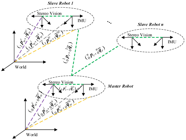 Figure 1
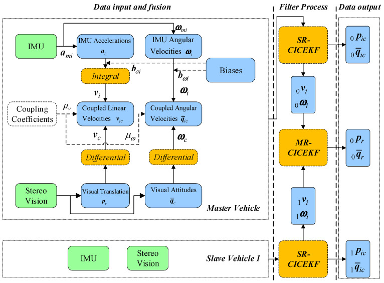 Figure 2
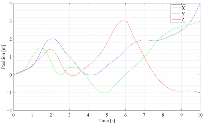 Figure 3
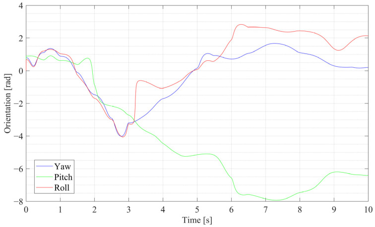 Figure 4
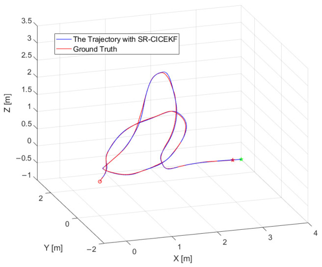 Figure 5
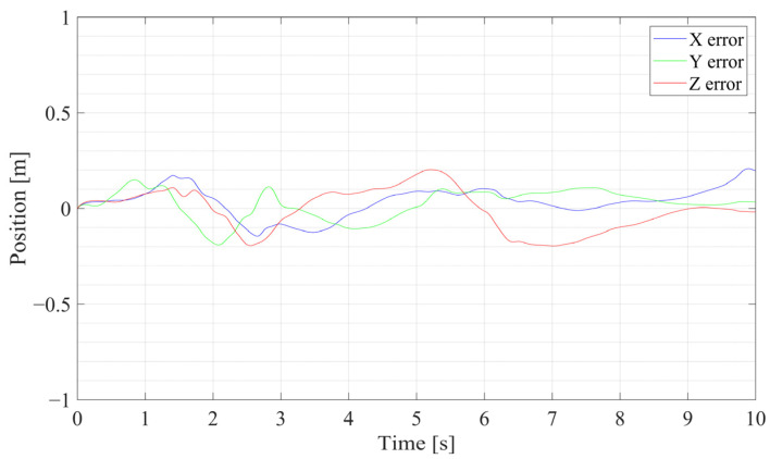 Figure 6
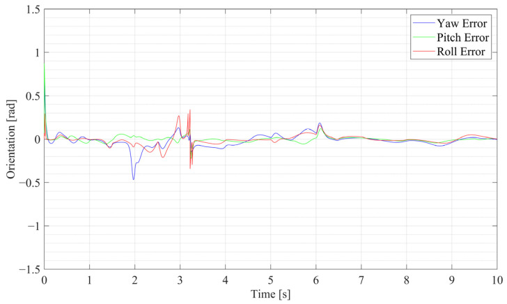 Figure 7
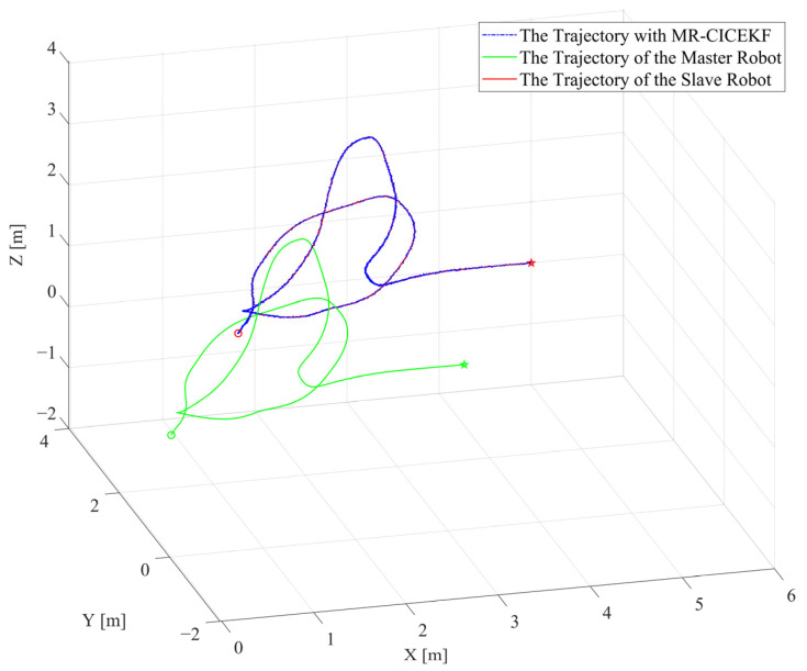 Figure 8
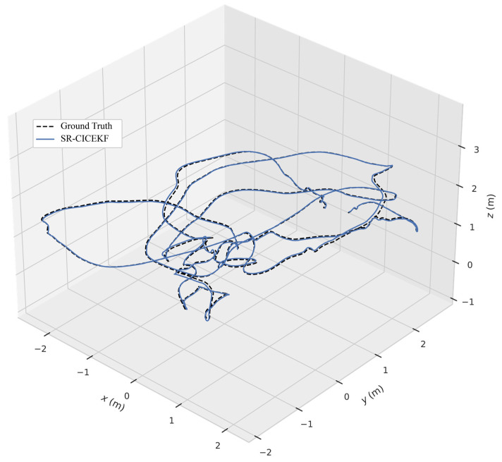 Figure 9
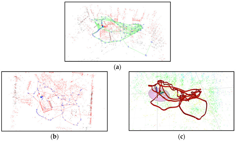 Figure 10
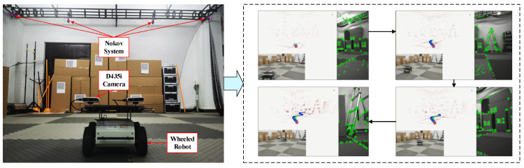 Figure 11
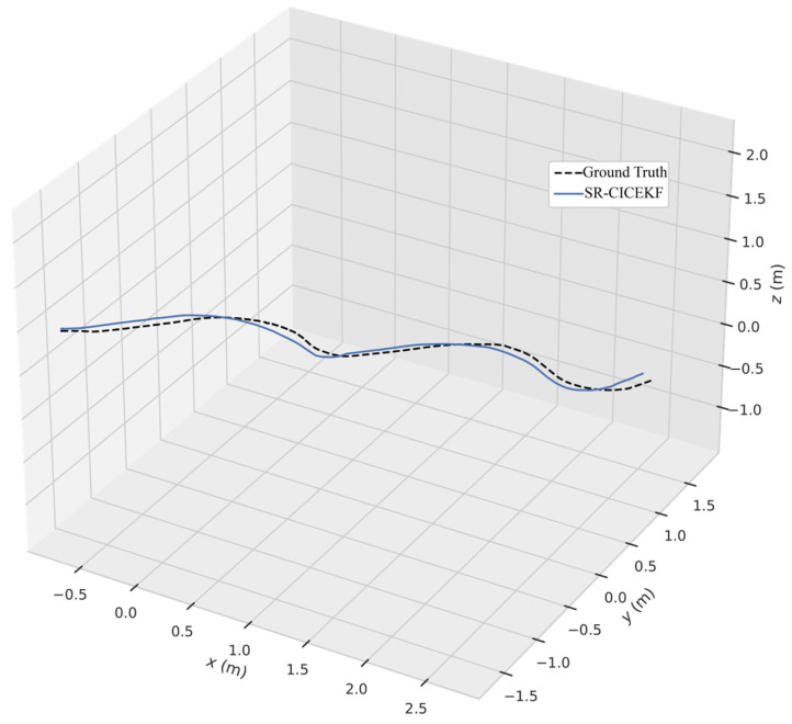 Figure 12
- —National Key Research and Development Program of China
- —Foundation for Innovative Research Groups of the National Natural Science Foundation of China
Peer Reviews
No public reviews on file for this paper yet. If you reviewed it on a platform where reviews are public (OpenReview, ICLR, NeurIPS, ICML), you can paste yours below so the community can read it here.
Videos
No videos yet. Explain this paper in a talk, walkthrough, or lecture? Add one.
Taxonomy
TopicsRobotics and Sensor-Based Localization · Advanced Vision and Imaging · 3D Surveying and Cultural Heritage
1. Introduction
1.1. Motivation
The autonomous localization of multiple robots working on ground and aerial space is well-explored and is achieved with different sensor setups such as visual measurement [1], GNSS (global navigation satellite system) [2], and visual–inertial equipment [3]. However, for search and rescue robots facing emergent or indoor situations [4,5], collaborative autonomous navigation under unknown and GNSS-denied environments [6] aiming for group closed-loop motion control [7,8] is still challenging due to the need for accuracy against environmental uncertainty. Visual–inertial approaches are popular for their robustness and real-time performance against interferences [9,10] to solve localization problems for both individual and group robots. Although the vision-based odometry and SLAM (simultaneous localization and mapping) methods have achieved great accuracy for their batch-optimization capability [11,12,13], the vision-only approaches are genuinely weak in solving the collaborative localization problem owing to the lack of a common world coordinate frame as an anchorage [14,15]. On the other hand, IMUs have good real-time responsiveness, while the inherent drift affects the long-term performance.
Therefore, it is necessary to explore approaches with an open and flexible data fusion framework to improve the accuracy of cooperative group localization, which can balance the instantaneity of the IMU sensors and the accuracy of visual measurement for collaborative agents under GNSS-restricted situations.
1.2. Related Work
The research on autonomous localization based on the data fusion of the IMU and visual measurement mainly focuses on tightly and loosely coupled approaches.
The tightly coupled methods are typically biased towards visual measurement when integrating the IMU’s real-time output from the gyroscope and accelerometer into the batch-optimization process. The state-of-the-art single-robot visual–inertial localization methods, such as ORB-SLAM v3 [16] and MSCKF 2.0 [17], have shown great robustness and accuracy. TH Nguyena et al. [18] proposed a two-step optimization-based collaborative visual–inertial range localization method that separately estimates the relative transformation and single-robot localization. Tian et al. [19] proposed a distributed multi-robot system for robust and dense metric semantic SLAM that detects loop closures and performs distributed trajectory estimation when communication among individuals is available. Though achieving great performance in the tests with the benefits of post-optimization, such tightly coupled methods usually lack both openness due to the fixed optimization structure and low real-time performance due to the high computing power demand. These result in inefficiency in dealing with uncertain topology and different mounted sensors of multi-agents.
Loosely coupled methods are naturally fit to perform relative localization due to their flexible algorithm structure and timeliness by emphasizing the IMU update [20]. The main weakness is their unsatisfactory accuracy owing to the inevitable drift of the IMU measurement, which should be carefully handled.
Kelly and Sukhatme [21] achieved the self-calibration of a monocular visual–inertial system with a specifically designed UKF (unscented Kalman filter). Following a similar approach, Weiss and Siegwart [22] introduced the estimation of the world coordinate frame drift of the visual measurement into a multi-level EKF (extended Kalman filter) for a better trajectory estimation for a single drone. Based on further research, Achtelik and Weiss [23] achieved the estimation of the relative configuration of two drones by utilizing a multi-level EKF to handle the loosely coupled visual–inertial data fusion. Researchers have introduced new filter techniques, such as the invariant EKF based on Lie algebra [24], the multi-state constraint Kalman filter [25], and the equivariant filter [26,27], into the trajectory estimation with visual–inertial equipment.
These loosely coupled methods usually treat visual measurement as a black box, thus achieving a flexible structure with great portability across different sensor setups. However, owing to only considering the update with IMU data on the acceleration and velocity levels, the final correction on the position level with the visual measurement result may lose accuracy when a sudden visual measurement instability is encountered.
1.3. Our Approach
This article presents a loosely coupled filter-based approach, the CICEKF, with two steps aiming for both the autonomous localization of a single robot and the collaborative estimation of relative multi-robot localization. The time complexity of the method is . The SR-CICEKF (single-robot CICEKF) step focuses on the fusion of the data on the stereo vision and IMU velocity levels from the integrated sensors for a robust locomotive estimation. The MR-CICEKF (multi-robot CICEKF) step fuses outcomes of the SR-CICEKF from multiple robots to estimate the real-time relative position and attitude from each slave robot to the master robot. The two steps can run separately as standalone filters or serially as a complete CICEKF. Furthermore, to demonstrate the feasibility of the CICEKF, the observability is proven.
This article is organized as follows: The design of the state vectors of the CICEKF is described in Section 2, a detailed description of the propagation and update processes of the filter is provided in Section 3, the local weak observability of the CICEKF is demonstrated in Section 4, simulation with quintic curves is presented in the Section 5, and real-world experiments were carried out and are analyzed in Section 6. The conclusions of this study are provided in Section 7.
2. Design of the State Vector
2.1. Definition of Variables
To focus the discussion on the filter-based data fusion process, the stereo vision is treated as black-box autonomous locomotion measurement equipment. It is assumed that each robot is equipped with an IMU-aided stereo-vision sensor suite, of which the relative position and attitude of the IMU and the cameras are already calibrated without further drifting. The locomotive variables and relative transformations are defined as shown in Figure 1, and the coordinate frames and the notation of variables used in this study are provided in Table 1.
The fixed index of the master robot is set as 0, and the indexes of the slave robots are numbered from 1 to . and represent the calibrated relative position and attitude, respectively, between the IMU and the stereo-vision coordinate frames of the -th robot. The -th robot’s linear translation and the rotation obtained from the black-box stereo vision are measured by referring to the world coordinate frame. and are the linear translation and the rotation of the IMU inspected in the world coordinate frame, respectively. The coupled position and attitude fusion results of each IMU–camera suite, i.e., and , are attached to its IMU coordinate frame to simplify the filtering process. The raw measurement outputs of the -th IMU are the linear acceleration and angular velocity , which are measured in its body-following coordinate frame. The relative configuration consists of the relative position and attitude between the -th slave robot and the master robot, which are and , respectively. The units used in this article are described in the SI. This design of the master/slave relationship among multiple agents allows for convenient modification of the topology under practical situations.
In this study, the drift of the vision’s world coordinate frame is not considered since it is slow enough to be treated as noise. Furthermore, all noise variables are modeled as a random walk·. The small-angle assumption is applied, which means letting the rotation angle be converted from be , and the error of is written as when [28].
2.2. Construction of the SR-CICEKF State Vector
From this point onwards, for the filter construction considering the IMU-aided stereo-vision suite of any single robot, the left corner markers are omitted for simplification, such as .
Thus, the vector with 29 elements representing the state of the SR-CICEKF is defined as follows:
where is the derivative of ; is integrated from , which possesses a bias ; is the angular velocity of the stereo vision body, which is inspected in the IMU coordinate frame rather than the vision coordinate frame; and is the angular velocity of the IMU body in its own coordinate frame with a bias . Additionally, there are and , where and are the measurement noises, and is the gravity vector with respect to the world coordinate frame.
2.2.1. Coupling Process for the SR-CICEKF
The independent coupling coefficients of the linear and angular velocities are and , respectively, ensuring adjustability while enhancing motion estimation accuracy without affecting observability.
The linear velocity coupling is straightforward and written as follows:
The coupling process of angular velocities cannot be conducted directly since the rotations of the IMU and vision body are inspected in different coordinate frames. Assuming , the following equations are obtained referring to [29]:
where is achieved by inspecting the rotation of the stereo vision body in the IMU coordinate frame, and is the -th power of , which denotes a unit quaternion scaling the rotation angle around the virtual axis with [30].
According to Appendix A, Equations (3) and (4), can thus be derived as follows:
where .
2.2.2. Simplification of the SR-CICEKF State Vector
To simplify the further discussion, the SR-CICEKF state vector in Equation (1) is rewritten as follows:
The corresponding derivatives are as follows:
where .
2.2.3. Error of the SR-CICEKF State Vector
The error state contributes to the propagation matrices and is essential for the filtering process. contains 27 elements, written as follows:
The update rate of this filter-based approach is determined by the IMU refresh rate. Thus, small high-order terms in the process can be omitted, such as , , and since the IMU can usually run faster than 100 Hz.
To build the connection from the state vector to the propagation process, the derivative form of should be inspected.
The derivative of the coupled translation error can be obtained directly as follows:
Let and , and according to achieved by following Appendix A, the equations are as follows:
where the higher-order terms are omitted.
According to Appendix A, the equations are as follows:
By subjecting Equation (11) to Equation (5), there is obtained as follows:
where is applied, and the high-order terms are disregarded.
Following the small-angle assumption, let , and there is as follows:
Similarly, there is as follows:
where and are applied.
Following the small-angle assumption, let , and there is as follows:
For other terms in the error state, there is no change compared to the state vector since they are obtained directly from the measurement. Therefore, there is as follows:
2.3. Construction of the MR-CICEKF State Vector
One primary purpose of this study is to achieve a relative configuration between two robots. Therefore, the IMU coordinate frame, which is inherent and fixed after calibration, is chosen as the anchorage to establish the filter. For the conditions with multiple robots running simultaneously, the relative configuration chain can be easily developed with a convenient adjustment to the topology.
The construction process of the MR-CICEKF state equations is partially similar to SR-CICEKF. The input of the MR-CICEKF is obtained from the output of SR-CICEKF, and the state vector with 19 elements is written as follows:
where and have been described previously, and are the IMU’s linear velocity and angular velocity obtained after applying the SR-CICEKF to the master robot’s sensor suite, respectively; and and are the outputs of the slave robot.
The derivative form of connects the variables in the state vector. The derivative of the relative translation is obtained as follows:
where is the relative linear velocity of the robots.
According to , the derivative of the relative rotation is written as follows:
2.3.1. Simplification of the MR-CICEKF State Vector
To simplify the further discussion, the MR-CICEKF state vector is rewritten as follows:
Additionally, there is . The derivatives of the relative motion variables are written as follows:
2.3.2. Error of the MR-CICEKF State Vector
contains 18 elements and is written as follows:
Following Appendix A, holds. According to , by omitting high-order terms, there is as follows:
where , and are applied.
Resembling the deduction process of Equations (11) and (12), the error of the relative rotation can be obtained as follows:
After applying the small-angle assumption, the result is as follows:
Since the linear and angular velocities are generated from the SR-CICEKF process, which can be seen as a measurement process, there is as follows:
2.4. Relationships Among the Variables in the CICEKF
By analyzing the construction of the state vectors, it can be concluded that the SR-CICEKF and the MR-CICEKF are tightly connected in the inheritance of variables and the synchronous update, which are assembled as an entire CICEKF process. The relationships among the variables in the CICEKF states are shown in Figure 2. The whole filter is divided into three parts: data preparation, filter process, and data output. The data preparation contains the data input and fusion for both the master and slave robots as individuals. The filter process is separated into two steps, which are SR-CICEKF and MR-CICEKF.
3. Propagation and Update of the CICEKF
The propagation process is key to connecting different layers of the filter. The update process introduces measurement data to correct the entire data fusion process.
3.1. Propagation and Measurement of the SR-CICEKF
3.1.1. Propagation of the SR-CICEKF
Let the continuous state transition matrix of the SR-CICEKF be and the continuous noise transition matrix be , which are constant over each integration time step. By linearizing the continuous-time errors of a CICEKF state, there is as follows [31]:
where the state noise vector is .
By applying Taylor’s formula, the discrete form of Equation (27) is as follows [31]:
where is the discrete form of , and the continuous noise covariance matrix is a diagonal matrix with being its discrete form.
By considering the first-order expansion, after computing the Jacobians to obtain , the expression of can be written as follows:
where .
Following Equations (28) and (29), can be obtained from , which is derived according to and written as follows:
3.1.2. Measurement of the SR-CICEKF
For an autonomous robot, the keyframes of the visual measurement can possess high localization accuracy for its post-batch optimization with visual features. Let the measurement vector of the SR-CICEKF at the -th step be with its error form as , where is the error of the linear position, the quaternion is the error of the rotation, is the error of the linear velocity, and is the error of the angular velocity. The measurement noise of the variables is simplified as .
Following and , the entire description of , , and based on variables in the error state vector of the SR-CICEKF can be deducted as follows:
In particular, the angular velocities of both sensors cannot be directly subtracted since they do not share the same coordinate frame. Therefore, is obtained indirectly from Equation (15) as follows:
The measurement matrix can be recovered from , which is written as follows:
where .
3.2. Propagation and Measurement of the MR-CICEKF
The processes of the propagation and measurement of the MR-CICEKF are similar to those of the SR-CICEKF and focus on relative motion estimation.
Following the deduction of the propagation matrix from Equation (27) to (28), let the noise vector of the state variables of the MR-CICEKF be . And the discrete relative state transition matrix is written as follows:
The discrete noise covariance matrix is , where there is as follows:
By defining the measurement noise vector of the MR-CICEKF as , let the measurement error of the MR-CICEKF at the -th step be , then, there is as follows:
After inspecting the relationship between the measurement and the desired output of the filter through , the measurement matrix can be deducted as follows:
3.3. Entire CICEKF Process
From the analysis above, it can be concluded that the CICEKF has two major EKF-based loops to update and correct the relevant states. The first loop, i.e., the SR-CICEKF, is shown in Algorithm 1, and the second loop, i.e., the MR-CICEKF, is shown in Algorithm 2, where and are the measurement noise matrices pre-established as described in [32,33], and are the Kalman gains, and are the prior covariance matrices of error, and and are the posterior covariance matrices of the error.
The first loop governs the propagation, measurement, and update of a single robot’s motion state by fusing the measurement data of the stereo vision and the IMU on the velocity level. The second loop is focused on the estimation of the relative positions and rotations of multiple slave robots with respect to the master robot. This dual-loop design keeps the independence of either algorithm for application in different motion estimation situations. When the two algorithms work serially to yield and successively, the entire algorithm complexity can be restricted to . Algorithm 1: SR-CICEKF Input: , , ;1While true do2Update , according to and ; ( Propagation process in Section 3.1.1)3Update ;4Update ;5Calculate according to ; ( Measurement process in Section 3.1.2)6Update the current state ;7Update ;8 ;9Output: . Algorithm 2: MR-CICEKF Input: , , , , ;1While true do2Update according to and ;3Update , according to and ; ( Propagation process in Section 3.2)4Update ;5Update ;6Calculate according to ; ( Measurement process in Section 3.2)7Update the current state ;8Update ;9 ;10Output: .
When updating each current state, the quaternion error is recovered from the angular errors using the following equations [28]:
4. Nonlinear Observability Analysis
4.1. Observability Analysis of the SR-CICEKF
When treating the filter as a nonlinear multi-input and multi-output system, its prerequisite for the filter to achieve correct estimation is that the system is observable. Researchers have proven that a filter possessing local weak observability can function properly, which is equivalent to the constructed observability matrix having full rank [21,34]. To simplify the discussion, a virtual measured angle velocity and its bias are assumed and partially coupled based on the IMU and visual measurement. Due to being in the filter state, and thus treated as paired with , this assumption does not affect the observability analysis. Thus, following Appendix A, the nonlinear measurement process of the SR-CICEKF can be expressed as follows:
where for a general unit quaternion , there is [21], and
The measurement functions for the SR-CICEKF are designed as , with , , , , , , , and .
Following the Lie derivative rules in Appendix A and in [21], the observability matrix is as follows:
where the matrices with the row and column indexes as subscripts do not contribute to the rank analysis.
To calculate the column rank, block Gaussian elimination can be applied. Once the corresponding block is an identity matrix, the relative column can be eliminated. Thus, only the last two columns are needed for the analysis and can be simplified as follows:
Therefore, if were non-zero, and any axis of the IMU was excited in any direction, has full column rank, and , thus, has full column rank. This means the SR-CICEKF has local weak observability [21,34]. The above conditions of achieving full rank are easily fulfilled during the application.
4.2. Observability Analysis of the MR-CICEKF
Resembling the previous analysis, the nonlinear system representing the measurement results of the MR-CICEKF can be expressed as follows:
The measurement functions for MR-CICEKF are designed as , with , , , , , and .
After applying Lie derivative rules, the observability matrix of the MR-CICEKF system is constructed as follows:
All the block columns in have full column rank when the single-robot measurement yields non-zero outcomes, which means that the system has local weak observability [21,34].
5. Data Test
Two sets of motion simulations were performed to test the feasibility of the CICEKF algorithm. The motion curve was chosen as quintic, which is convenient for calculating the linear accelerations.
5.1. SR-CICEKF Simulation Test
To simplify the simulation for an individual sensor suite, the coordinate frames of the IMU and the stereo vision are assumed to coincide, and the biases are omitted. Once the parameters of the quintic curve are confirmed, the position coordinates of the curve can be treated as the position ground truth. By analyzing the projections of the curve on the three standard planes, the roll, pitch, and yaw orientations of the adjacent points can be achieved by allocating the starting and ending points, which yields the ground truth of the orientation. Thus, the ideal linear acceleration, linear velocity, and angular velocity data can be differentiated from the position and orientations, which are utilized as the filter input after being corrupted with Gaussian noise.
The position and orientation curves of the generated quintic trajectory across all three axes are shown in Figure 3 and Figure 4, respectively. It should be noted that the change in the trajectory is designed in a short time span of 10 s with a 1000 Hz update rate, which means the change in simulation data is quite fast; for example, the maximum angular velocity is over 6 rad/s, and the max linear acceleration is over 11 m^2^/s.
can be asymptotically stable after a complete run with the randomized initial values. By reusing the stabilized in other runs, the initial convergence of the filter process can be greatly boosted. is designed as a skew-symmetric matrix containing small random values. The coefficients are set as and . The initial position and orientation are set as [0, 0, 0].
The three-dimensional position curves of the SR-CICEKF simulation are shown in Figure 5, with the circle mark as the starting point and the star markers as the ending points. The errors between the virtual measurement values and the filtered values of the position and orientation are shown in Figure 6 and Figure 7, respectively. The statistical results of RMSE, mean errors, and STD of the norm errors involving the three axes of the position and the orientation are listed in Table 2.
By inspecting the curves and the statistical values, it can be concluded that the SR-CICEKF quickly converges under severe data changes, while it does not need careful parameter tuning for the first estimation of . This indicates that the filter is robust, and the observability of the fusion process is identified indirectly.
5.2. MR-CICEKF Simulation
The goal of the simulation is to estimate the relative translation and rotation between the master and slave robots. The MR-CICEKF simulation utilizes the same quintic data as the target trajectories of both the master and slave robots. The absolute relative translation of the two robots is set as [1, 1, 1], and the relative rotation is set as [0, 0, 0]. The MR-CICEKF is tested independently of the SR-CICEKF. Thus, the performance of the MR-CICEKF is not affected by the possible inaccuracy produced by the SR-CICEKF process. The configurations of and are similar to the SR-CICEKF simulation, and the simulation input is corrupted with Gaussian noise.
Figure 8 depicts the three-dimensional position curves of the MR-CICEKF simulation, containing the ground truth of the master and slave robots’ trajectories, and the filtered slave robot trajectory, which is achieved by adding the estimated and to the master trajectory. The circle marks are the starting points, and the star markers are the ending points. The statistical values of RMSE, mean errors, and STD of the norm errors involving the three axes of the position and the orientation obtained after comparing the ground truth with the filtered slave robot trajectories are listed in Table 3.
The statistical values indicate that the final error is similar to the small white noise added. Thus, it can be concluded that the MR-CICEKF possesses good estimation accuracy, while the main error is caused by eliminating high-order terms during the state transition. This feature can significantly simplify further application since the MR-CICEKF contributes little error to the entire CICEKF process.
5.3. Dataset Test
To further analyze the performance of the CICEKF in real-world scenarios, a test was performed with the EuRoC dataset. The SR-CICEKF part is tested solely since the MR-CICEKF already showed great performance. The state-of-the-art visual SLAM method, ORB-SLAM V3 [16], was utilized as the visual black box measurement algorithm. The SR-CICEKF runs at 200 Hz, which is synchronous with the IMU update rate of the dataset. By employing EVO tools [35], the RPE features of the trajectories can be directly digitized.
The stereo vision of ORB-SLAM V3 runs at 20 Hz, and all measurement frames were treated as keyframes. The coefficients were set as and . The initial covariance matrix was tuned following the aforementioned strategy. The SR-CICEKF, stereo ORB-SLAM V3, and its variant, along with the stereo MSCKF [17], were carried out with the room dataset of EuRoC under the same computer configuration. Figure 9 shows the comparison of the estimation trajectories of the SR-CICEKF and the ground truth. Figure 10 shows the dataset test scenarios of the algorithms separately. The RPE comparison results between each algorithm with the ground truth achieved by utilizing the EVO tools are listed in Table 4.
From the comparison, it can be concluded that by fusing IMU information and the pure visual black box measurement with the proposed SR-CICEKF algorithm, the accuracy has been greatly improved. Although the accuracy of the approach does not reach that of the optimization-based method, the fusion computational complexity is as low as . This can benefit the fusion with other visual measurement algorithms to improve the performance of trajectory estimation without affecting the computing efficiency. Furthermore, it can be combined with MR-CICEKF for the simultaneous estimation of multiple agents’ trajectories and collaborative configurations.
6. Experiments
Two experiments were designed to focus the discussion on the feasibility of the proposed method. Firstly, the Intel RealSense D435i, which contains a stereo set of cameras and an IMU, was mounted on a wheeled robot that performs locomotion. The SR-CICEKF estimated the locomotive trajectory while the ground truth was measured by the NOKOV motion capture system. Then, the D435i camera data were utilized for collaborative loco-motion estimation. The experimental scenarios (Supplementary Materials) are shown in Figure 11.
For both parts of the CICEKF, the black-box stereo visual algorithm is ORB-SLAM V3 operating at 30 Hz, while the IMU update rate is set to 200 Hz. The calibration of the cameras and IMUs was conducted using Kalibr tools [36] to obtain the intrinsic and extrinsic parameters and the fixed configuration of the integrated sensors.
During the experiment, we noticed that ORB-SLAM V3 and its IMU variant might not be stable under our experimental conditions due to the calibration accuracy and the IMU lacking sufficient excitation, since we used a slow ground vehicle as the motion platform. Therefore, to demonstrate the performance of the SR-CICEKF, the estimated trajectory was compared with that of stereo ORB-SLAM V3 and stereo MSCKF. The coefficients were set as and . The comparison of the measured trajectory and the ground truth is shown in Figure 12. The RPE comparison results between each algorithm with the ground truth in a real scenario are listed in Table 5.
For the MR-CICEKF experiment, the two D435i cameras were calibrated with Kalibr tools to achieve a fixed relative configuration as both the ground truth and the initial guess of the filter. The relative configuration estimation of the MR-CICEKF was compared with the ground truth. The norm errors of the relative configuration estimation are listed in Table 6.
From the experimental results, it can be concluded that the proposed algorithm can not only improve the accuracy of pure visual measurement algorithms but also reliably estimate the relative configuration of multiple robots.
7. Conclusions
This study introduces a novel motion estimation approach with a loosely coupled and dual-step structure for the autonomous and collaborative localization of multiple locomotive robots. Both steps of the algorithm can run standalone, serially, or in parallel while maintaining a computational complexity of , which allows for convenient improvement to pure vision measurement techniques after introducing an IMU. Both the simulations and experiments demonstrate that fusing data on the velocity level without post-optimization greatly contributes to the robot trajectory estimation accuracy. Due to current experimental limitations, further research will be focused on systematically examining how the coupling coefficients affect filter performance and stability across various integrated sensors and high-speed motion units.
The reference list from the paper itself. Each links out to its DOI / PubMed record.
- 1Servières M. Renaudin V. Dupuis A. Antigny N. Visual and Visual-Inertial SLAM: State of the Art, Classification, and Experimental Benchmarking J. Sens.20212021205482810.1155/2021/2054828 · doi ↗
- 2Sun Z. Gao W. Tao X. Pan S. Wu P. Huang H. Semi-tightly coupled robust model for GNSS/UWB/INS integrated positioning in challenging environments Remote Sens.202416210810.3390/rs 16122108 · doi ↗
- 3He M. Zhu C. Huang Q. Ren B. Liu J. A review of monocular visual odometry Vis. Comput.2020361053106510.1007/s 00371-019-01714-6 · doi ↗
- 4Elamin A. El-Rabbany A. Jacob S. Event-Based Visual/Inertial Odometry for UAV Indoor Navigation Sensors 2024256110.3390/s 2501006139796852 PMC 11722967 · doi ↗ · pubmed ↗
- 5Hu C. Huang P. Wang W. Tightly coupled visual-inertial-UWB indoor localization system with multiple position-unknown anchors IEEE Robot. Autom. Lett.2023935135810.1109/LRA.2023.3328367 · doi ↗
- 6Tonini A. Castelli M. Bates J.S. Lin N.N.N. Painho M. Visual-Inertial Method for Localizing Aerial Vehicles in GNSS-Denied Environments Appl. Sci.202414949310.3390/app 14209493 · doi ↗
- 7Nemec D. Šimák V. Janota A. HrubošM. BubeníkováE. Precise localization of the mobile wheeled robot using sensor fusion of odometry, visual artificial landmarks and inertial sensors Robot. Auton. Syst.201911216817710.1016/j.robot.2018.11.019 · doi ↗
- 8Li Z. You B. Ding L. Gao H. Huang F. Trajectory Tracking Control for WM Rs with the Time-Varying Longitudinal Slippage Based on a New Adaptive SMC Method Int. J. Aerosp. Eng.20192019495153810.1155/2019/4951538 · doi ↗