Fall and Winter Temperatures, Together with Spring Temperatures, Determine the First Flowering Date of Prunus armeniaca L
Di Tang, Brady K. Quinn, Yunfeng Yang, Liang Guo, David A. Ratkowsky, Peijian Shi

TL;DR
This study shows that fall and winter temperatures, along with spring temperatures, help predict when apricot trees will first bloom in spring.
Contribution
The study demonstrates that fall and winter temperatures significantly reduce prediction errors in bloom timing when combined with the ADP method.
Findings
The ADP method had the lowest prediction error for apricot first flowering date.
Fall and winter temperatures explained 96% of the remaining prediction error from the ADP method.
Including temperature predictors reduced the root mean square error to 0.6162 days.
Abstract
Chilling and spring temperature accumulation are both considered key factors determining the timing of the spring bloom in many flowering plants. The accumulated developmental progress (ADP) method predicted the first flowering date (FFD) of a species of Rosaceae well in a previous study. However, whether this approach can be applied to other species, and whether the prediction errors in FFD based on the ADP method can be further accounted for by fall and winter temperatures (FWTs), remains unknown. The ADP method and two others were tested using a 39-year apricot FFD data series. The goodness of fit obtained with each method was assessed using the root mean square error (RMSE) between the observed and predicted FFDs. We used the residuals obtained using the ADP method as a response variable to fit generalized additive models (GAMs) including six FWTs as predictors. The GAMs generated…
Genes, proteins, chemicals, diseases, species, mutations and cell lines named across the full text — each resolved to its canonical identifier and authoritative record.
Click any figure to enlarge with its caption.
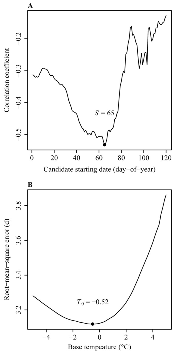 Figure 1
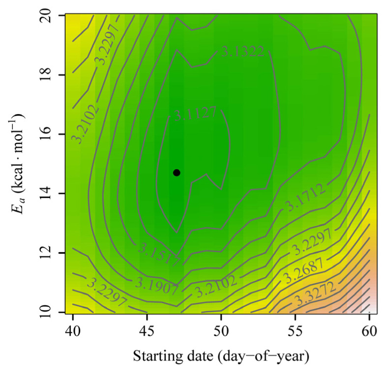 Figure 2
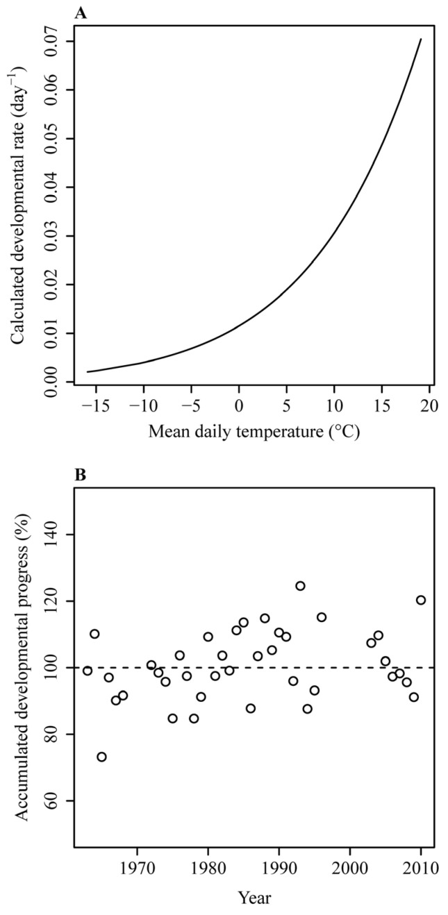 Figure 3
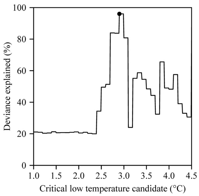 Figure 4
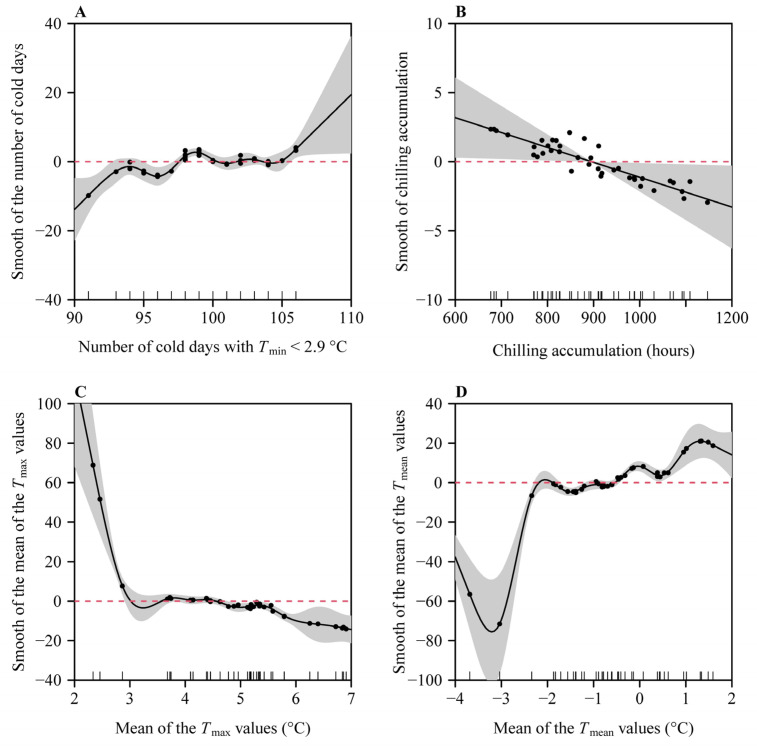 Figure 5
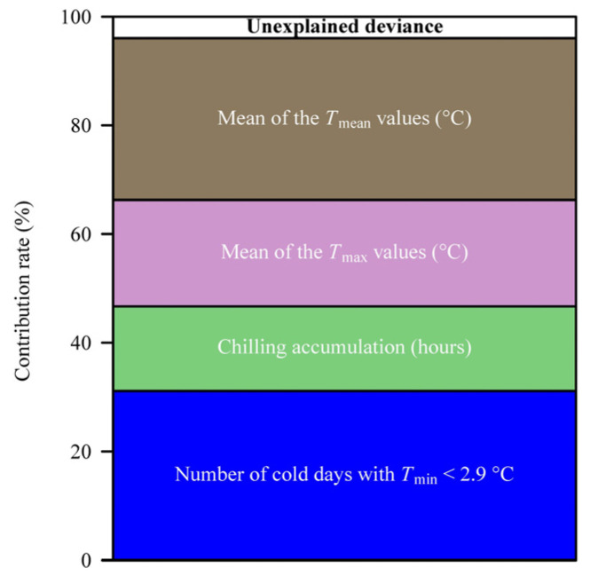 Figure 6
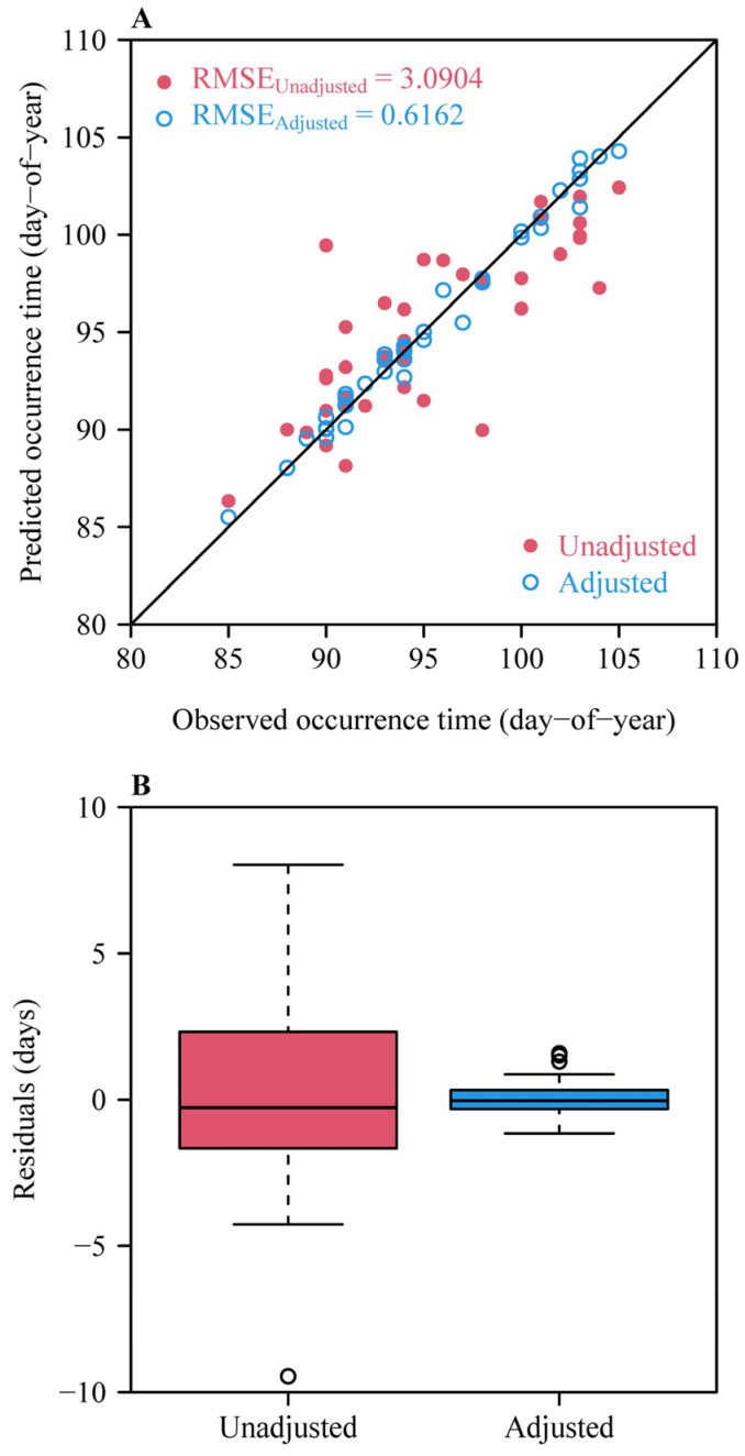 Figure 7
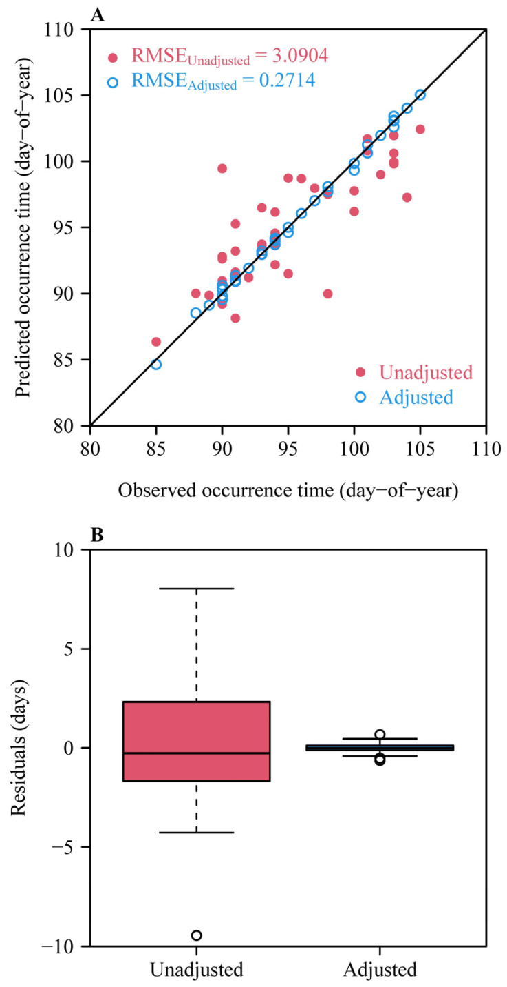 Figure 8
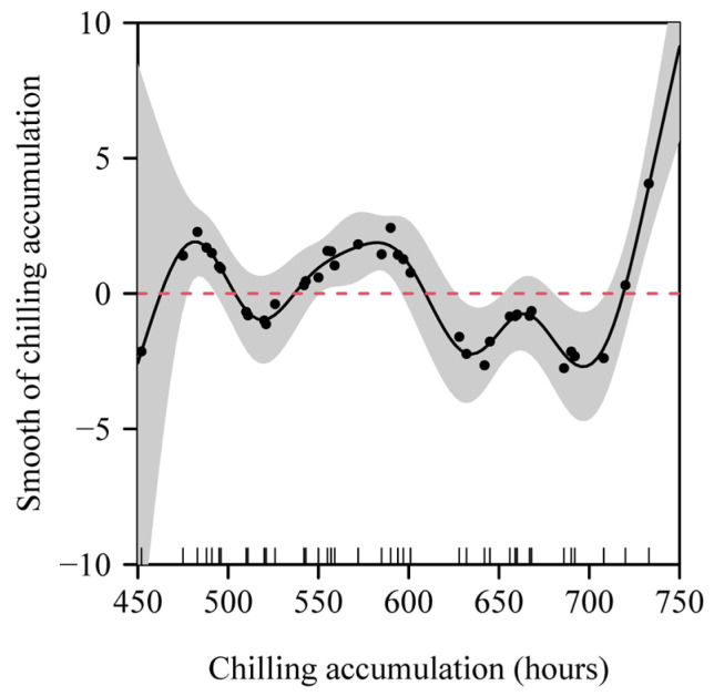 Figure 9
- —National Natural Science Foundation of China
Peer Reviews
No public reviews on file for this paper yet. If you reviewed it on a platform where reviews are public (OpenReview, ICLR, NeurIPS, ICML), you can paste yours below so the community can read it here.
Videos
No videos yet. Explain this paper in a talk, walkthrough, or lecture? Add one.
Taxonomy
TopicsPlant Physiology and Cultivation Studies · Horticultural and Viticultural Research · Plant Reproductive Biology
1. Introduction
Phenology is closely associated with the services and functioning of ecosystems involved in agriculture, fishery, forestry, and horticulture [1,2]. Global climate warming has strongly impacted the timing of many phenological events of animals and plants [3,4,5]. Such shifts can lead to a mismatch between the phenological occurrence of plants and that of herbivores, as well as a subsequent mismatch between herbivores and carnivores [6]. Spring phenology is always a focus of phenological investigation because the growth and development of many poikilotherms and plants are temperature-dependent, and such organisms usually break dormancy and diapause in response to gradually increasing daily air temperatures in this season in the temperate zone of the Northern Hemisphere [3]. The currently popular viewpoint is that the timing of spring phenology is determined both by fall and winter low temperatures and spring mean temperatures [4,7]. The spring phenology of plants can be advanced by increasing spring temperatures but delayed by increasing fall and winter temperatures due to the reduction in fall and winter chilling accumulation [4]. The extent of fall and winter chilling accumulation has always been considered to have a significant influence on the spring phenology of plants, such as the timing of bud sprouting, flowering, and leaf unfolding, and several models of these relationships have been proposed [8,9]. Relative to the influence of spring temperatures, the influence of fall and winter temperatures (FWTs) on the occurrence time of spring phenological events has seldom been tested, with the exception of a few studies [10,11,12,13]. Most prior studies hypothesized that FWTs make a smaller contribution to the occurrence time of spring phenology than that of spring temperatures and that the relative contributions of these predictors are species-specific [10]. However, whether this hypothesis holds true generally remains unknown.
The spring phenology of plants, especially the timing of key developmental events in early spring, is related to the breaking of two stages of dormancy: endo-dormancy that can only be broken by a certain chilling accumulation and eco-dormancy that can only be broken by a certain heat accumulation [14,15]. Chilling accumulation is considered to play a critical role in breaking endo-dormancy, and after the completion of endo-dormancy, the accumulation of spring effective temperatures is considered to play a critical role in breaking eco-dormancy [14,16,17]. Significant interspecific variation in chilling requirements (CRs) and heat requirements (HRs) has been documented in apricot (Prunus armeniaca L.) [18]. Studies quantified CRs across cultivars as ranging from 596 to 1266 chilling units, revealing a negative correlation between CRs and HRs. This variability underscores the necessity of cultivar-specific agroclimatic assessments, particularly under climate change scenarios where incomplete CRs fulfillment may lead to erratic flowering and yield instability [19]. For the latter process (i.e., the breaking of eco-dormancy), the effect of spring temperatures on the time of occurrence can be clearly explained by experimental evidence from thermal biology in arthropods and plants ([20,21,22] and references therein). The effect of temperature (T) on the developmental rate (denoted as r, i.e., the reciprocal of the developmental duration for completing a specific developmental stage, which represents the developmental progression per unit time) is a left-skewed bell-shaped curve. At low temperatures, r exponentially increases with T; at moderate temperatures, r increases approximately linearly with T; at high temperatures, r steeply decreases with T [23,24,25]. There are many mathematical models available that describe the temperature-dependent developmental rate of arthropods and plants [20,21,26,27]. In early spring, daily mean temperature (denoted as Tmean) is usually lower than 20 °C, so the temperature-dependent development rate can be approximated by a linear or exponential equation [23,24,25,28]. Because the developmental rate does not decrease in low and mid-temperature ranges, some investigators even use the logistic equation to describe the effect of temperature on developmental rate [29] and then apply this approach to account for the effect of spring temperatures (referred to as forcing requirement in many studies on phenology) on the breaking of eco-dormancy [30]. Regardless of whether the developmental rate–temperature relationship is thought of as a straight line or a curve, the timing of a particular phenological event can be predicted by calculating the cumulative developmental rates associated with the daily Tmean values in a period from a starting date to the occurrence time, adding up to 100% [11,12,31]. Using some optimization methods to minimize the root mean square error (RMSE) between the observed and predicted occurrence dates, the starting date (in day-of-year) and the parameters of the developmental rate equation can then be determined. This approach is referred to as the accumulated developmental progress (ADP) method [11,12]. The ADP method was found to be better than the traditional accumulated degree-day (ADD) method. However, prior studies have usually reported large prediction errors for both the ADD and ADP methods, reflected by their RMSE ranging between 2 and 5 days between the observed and predicted occurrence times [10,11,12,32,33]. Although some mathematical models have already been proposed to describe the effect of fall and winter low temperatures on the break of endo-dormancy, these methods are usually based on species-specific experiments, and the model parameters lack generalizability to other species [13,14,16,30]. In addition, these models usually require that the parameters of auxiliary models are predetermined, which introduces a certain degree of subjectivity into their determination [13]. It should also be noted that the prediction errors resulting from such models are large, probably because of small sample size (i.e., the number of years for which there are phenological records) or probable problems inherent in these methods themselves.
The main reason that temperature-dependent developmental rate models have large prediction errors is that those models neglect the effect of FWTs on the break of endo-dormancy; further, the main reason that the existing models that consider the effects of fall and winter temperatures and spring temperatures on spring phenology also have large prediction errors is that the mechanisms by which FWTs impact phenology have been not as clearly elucidated as those of spring temperatures have so far [13]. Many models of the effect of FWTs on the break of endo-dormancy lack sufficiently convincing experimental evidence to be used as a general tool [13,14,16,30]. In this context, Shi et al. [11] proposed a method to solve this problem based on the first flowering date (FFD) time series of a species of Rosaceae, the cherry Prunus × yedoensis Matsum. First, the ADP method was used to calculate the predicted occurrence dates (in day-of-year). Second, the residuals calculated between the observed and predicted occurrence dates were further analyzed using three fall and winter low temperature measures: (i) the number of cold days with daily minimum temperature (Tmin) ≤ −5.6 °C; (ii) the mean of the Tmin values from 1 November of the preceding year to the starting date for the ADP method; and (iii) the minimum annual temperature. Using the above protocols, the RMSE value for predicting the FFD of P. yedoensis decreased from 4.29 to 2.80 days. However, two issues were not addressed by this approach. One is whether the protocols proposed by ref. [11] apply to the FFD of other species, and another is whether the prediction error can be further decreased by introducing other measures of FWTs into predictive models; e.g., the daily maximum temperatures (Tmax) in fall and winter that have been largely neglected in prior work. For instance, increased fall and winter Tmax likely leads plants to finish accumulating effective temperatures earlier, which might lead to spring phenological events happening sooner in the year.
In the present study, we used a 39-year FFD time series of P. armeniaca at a representative site to test the validity of the ADP method and examine whether FWTs, including the daily minimum, maximum, and mean temperatures in fall and winter, as well as the number of cold days with Tmin less than a certain low temperature in the fall and winter seasons, can significantly influence the prediction of FFD in this species of Rosaceae.
2. Materials and Methods
2.1. First Flowering Date Records and Climate Data
First flowering date (FFD) data for P. armeniaca came from the Chinese Phenological Observation Network, which were recorded at the Summer Palace of Beijing, China (39°54′38″ N, 116°8′28″ E, 50 m above sea level) from 1963 to 2010, with the exceptions of 1969–1971 and 1997–2002 [34]. In total, there are 39 years of FFD records in the data set. Daily climate data of Beijing from 1962 to 2010 came from the China Meteorological Data Service Centre (https://data.cma.cn/en; accessed on 4 April 2014). The FFD and climate data are included in the R package “spphpr” (v1.1.4) [35].
2.2. Methods for Quantifying the Effect of Spring Temperatures on Phenological Occurrence Date
2.2.1. Accumulated Degree Days (ADD) Method
This method is based on the hypothesis that the development rate, r, increases approximately linearly with temperature, T, which is expressed as a linear equation:
where a and b are constants to be estimated. The temperature associated with r = 0 is defined as the lower developmental threshold temperature (or the “biological zero degree”), denoted as T0, where . When T < T0, r is considered to be zero. Equation (1) can alternatively be written as follows:
where k is the accumulation of effective temperatures (i.e., temperatures greater than the biological zero degree) required for completing a particular developmental stage, and D is the developmental duration, i.e., the reciprocal of r. In this representation, it is apparent that k = 1/b. It must be noted that r and k in Equations (1) and (2) are calculated as functions of constant experimental temperature. However, daily air temperatures in nature are variable. To capture this, Equation (2) can thus be rewritten as follows:
where the subscript i represents ith year, S represents the starting date (in day-of-year) when the accumulation of effective temperatures starts, E_i_ represents the actual occurrence date of a particular phenological event, the subscript j represents the jth day (day-of-year), and T_ij_ represents the daily mean temperature of the jth day of the ith year. If one assumes that there are n-year phenological records, then there is a series of k_i_ values, i.e., k1, k2, k3, …, k_n_.
In theory, the accumulation of effective temperatures required to complete development to a particular stage or phenological event’s occurrence is a constant value across different years. However, the k_i_ values calculated from empirical observations show some variation across different years. The mean of the k_i_ values, denoted as , is regarded as the expected required accumulation of effective temperatures. Here, S and T0 are unknown parameters that need to be estimated. The following protocols for determining the two parameters were recommended by Aono [33]. First, the mean value of the daily mean temperatures between the starting date of observations and the observed occurrence date is hypothesized to be negatively correlated with the observed occurrence date. This means that a higher mean temperature during the developmental period can result in the phenological event occurring at an earlier date. A group of candidate S values are provided, and the value associated with the lowest correlation coefficient between the mean of the daily mean temperatures from the starting date and the observed occurrence date is determined as the estimated value of S. Second, a group of candidate T0 values are provided. Using each candidate T0 value, the predicted occurrence date in the ith year is determined by the following steps. When (where F_i_ > S), F_i_ is the predicted occurrence date in the ith year; when and , the trapezoid method [32,36] is used to determine the predicted occurrence date in the ith year. The root mean square error (RMSE) calculated between the observed and predicted occurrence dates is then used to determine the numerical value of T0, such that the candidate T0 value associated with the lowest RMSE is selected as the estimated value of T0.
2.2.2. Accumulated Days Transferred to a Standardized Temperature (ADTS) Method
This method is based on the hypothesis that r increases approximately exponentially as T (in K) increases, which can be expressed using the Arrhenius equation [11,33,37]:
where A is a pre-exponential constant to be estimated, B = log(A), E_a_ is the activation free energy (in kcal∙mod^−1^) of a biochemical reaction controlling developmental progression, and R is the universal gas constant (=1.987 × 10^−3^ kal∙mol^−1^∙K^−1^). In practice, to reduce the value of B during parameter estimation, the pre-exponential constant is multiplied by 10^12^, i.e., .
According to the definition of r, it represents the developmental progress per unit time (e.g., per day) and is the reciprocal of the developmental duration D, i.e., r = 1/D. Let T_s_ represent a standard temperature (in K, e.g., 25 °C = 298.15 K) and r_s_ represent the developmental rate at this standard temperature. Let r_j_ represent the developmental rate at T_j_, an arbitrary absolute temperature (in K). Given that , it follows that
where is termed the number of days transferred to a standardized temperature (DTS) [33,37]. If one replaces T_j_ in Equation (5) with T_ij_ (i.e., the daily mean temperature of the jth day of the ith year), then the annual accumulated DTS of the ith year (denoted as U_i_) equals
As for the accumulation of effective temperatures described above, in theory, the annual accumulated DTS is a constant value, but calculated U_i_ values exhibit some variation across different years. The mean of the U_i_ values, denoted as , is regarded as the expected value. Here, S and E_a_ are unknown parameters that need to be estimated. The following protocols to determine the two parameters have been recommended in previous studies [33,37]. First, different combinations of the candidate S values and candidate E_a_ values are provided. Using each combination, the predicted occurrence date in the ith year is then determined by the following steps. When (where F_i_ > S), F_i_ is the predicted occurrence date in the ith year; when and , the trapezoid method [32,36] is used to determine the predicted occurrence date in the ith year. The RMSE calculated between the observed and predicted occurrence dates is then used to determine the numerical values of S and E_a_. Specifically, the combination of the candidate S and E_a_ values that is associated with the lowest RMSE is selected as that with the estimated values of S and E_a_. It should be noted that the ADTS method only applies when the temperature-dependent developmental rate equation is expressed as the Arrhenius equation.
2.2.3. Accumulated Developmental Progress (ADP) Method
This method permits the user to predict the occurrence date using any defined temperature-dependent developmental rate equation, denoted as , where P represents the vector of the model parameter(s). In this method, when the annual accumulated developmental progress (i.e., the accumulated developmental rates) reaches 100%, the phenological event is predicted to occur for each year [11,12,31,38]. Let V_i_ represent the annual accumulated developmental progress in the ith year, which equals
In theory, all V_i_ values are a constant value of 100%, although actual calculated V_i_ values do vary somewhat across different years. The following approach is used to determine the predicted occurrence date. When (where F_i_ > S), F_i_ is the predicted occurrence date in the ith year; when and , the trapezoid method [32,36] is used to determine the predicted occurrence date in the ith year. When the starting date (S) and are known, the model parameters can be estimated using the Nelder–Mead optimization method [39] to minimize the RMSE between the observed and predicted occurrence dates, i.e.,
where represents the predicted occurrence date in the ith year. Because S is not determined in the model fitting here, a group of candidate S values (in day-of-year) need to be provided. Assuming that there are m candidate S values, i.e., S1, S2, S3, ∙∙∙, S_m_, then for each S_q_ (where q ranges between 1 and m), a vector of the estimated model parameters, , can be generated by minimizing RMSEq using the Nelder–Mead optimization method [39]. Then, the associated with min{RMSE_1_, RMSE_2_, RMSE_3_, ∙∙∙, RMSEm} is finally the target parameter vector.
2.3. Methods for Quantifying the Effect of Fall and Winter Temperatures (FWTs) on Occurrence Date
As described above, the ADD, ADTS, and ADP methods were used to predict the first flowering dates of apricots, and the method associated with the lowest RMSE between the observed and predicted occurrence dates was selected for use in subsequent analyses. The residuals between the observed and predicted occurrence dates were calculated and then treated as the response variable, y, in analyses of the effects of fall and winter temperatures (FWTs) on occurrence date prediction. The present study tested the following six FWT measures as potential predictors: the number of days with daily minimum temperature ≤ a critical low temperature (x1), the number of chilling hours (x2), the mean value of the daily minimum temperatures (x3), the mean value of the daily maximum temperatures (x4), the mean value of the daily mean temperatures (x5), and the minimum value of the daily minimum temperatures (i.e., the minimum annual temperature, x6); all these predictors were calculated from 1 November of the preceding year to the starting date. Generalized additive models (GAMs) [40,41,42] with different candidate combinations of the above predictors were generated and compared to examine the relationships of y to the above predictors (Table 1).
A GAM is a non-parametric fitting method for multiple predictors, and does not require that the influence of each predictor on the response variable is known in advance. Using the partial residual plots generated during GAM fitting [40,41,42], the influence of each predictor on the response variable can be readily observed. When the mechanisms by which the various FWT measures influence the occurrence date are not known, it is feasible to use GAMs to explore the forms (linear or non-linear performance) of the relationships between those predictors and the occurrence date. We selected the best model among the candidate GAMs that we tested as the one that had the highest percentage of deviance explained (%), provided that all smooth terms were significant at the 0.05 level. In addition, Akaike’s information criterion (AIC) [43,44] was used to compare models. The model with the lowest AIC was selected as the best, as the AIC value calculated for a model reflects the trade-off between its goodness of fit (decreases AIC) and model structural complexity (increases AIC).
The critical low temperature used to calculate the observed x1 was determined by selecting the critical low temperature associated with the largest percentage of deviance explained among a set of candidate critical low temperatures. The accumulated chilling hours (ACH) in the ith year (observed x2) were calculated using the Chilling Hours model [8,45,46]:
where the first term on the right-hand side of Equation (9) represents the ACH from 1 November to 31 December of the preceding year, and the second term on the right-hand side of Equation (9) represents the ACH from 1 January to the starting date. The term is the indicator function, which equals
Here, is the temperature of the wth hour of the jth day of the ith year, which was calculated using the following formula [47]:
where Tmin and Tmax represent the daily minimum and maximum temperatures, respectively, and w ranges from 1 to 24.
To quantify the contribution rate (CR) of each predictor variable to the deviance explained by fitting a GAM with z variables (z ≤ 6) to the data, the following approach was taken [48]:
where CRi represents the contribution rate of the ith variable, DEj represents the proportion of the deviance explained by the GAM dropping the jth variable, and DE_0_ represents the proportion of deviance explained by the GAM using all z variables simultaneously (presumed to have highest predictive power).
All calculations were carried out using R (v4.3.1) [49]. The ADD, ADTS, and ADP methods were carried out with the “spphpr” package (v1.1.4) [35], whilst the GAMs were carried out with the “mgcv” package (v1.9-1) [42,50].
3. Results
For the accumulated degree-days (ADD) method, the estimated starting date (S) was day-of-year (DOY) 65, which was associated with a minimum correlation coefficient (between the occurrence date and the mean of the daily mean temperatures from the candidate starting date to the occurrence date) of −0.53 (Figure 1A). Using this method, the estimated base temperature (i.e., the biological zero degree) was −0.52 °C (Figure 1B), and the root mean square error (RMSE) was 3.1189 days. For the accumulated days transferred to a standardized temperature (ADTS) method, the estimated S was DOY 47, the estimated E_a_ was 14.7 kcal∙mol^−1^, and the RMSE was 3.0932 days (Figure 2). For the accumulated developmental progress (ADP) method, the estimated S was DOY 47, the estimated values of B and E_a_ were −4.38 and 15.04 kcal∙mol^−1^, respectively, and the RMSE was 3.0904 days. The predicted temperature-dependent developmental rate curve in the form of the Arrhenius equation (i.e., Equation (4)) based on the ADP method, and the deviation of the calculated developmental progress from the theoretical prediction of 100% across different phenological years, are shown in Figure 3. Among the three methods, the ADP method had the lowest RMSE value.
When the critical low temperature was equal to 2.9 °C, the percentage of deviance explained by the generalized additive model (GAM) reached the maximum value of 96% (Figure 4). Analyses using GAMs showed that the number of days with a daily minimum temperature ≤ 2.9 °C (x1), the number of chilling hours (x2), the mean value of the daily maximum temperatures (x4), and the mean value of the daily mean temperatures (x5) significantly influenced the residuals between the observed occurrence dates and those predicted by the ADP method (Table 1; Figure 5). As the number of days with a daily minimum temperature ≤ 2.9 °C and the mean value of the daily mean temperatures increased, the magnitude of the residuals overall increased; conversely, as the fall and winter chilling hours and the mean value of the daily maximum temperatures increased, the magnitude of the residuals overall decreased (Figure 5). Figure 6 shows the contribution rates of these four variables to deviance explained by the best GAM.
After fitting GAMs considering the influences of the above four fall and winter temperature measures on the residuals between the observed occurrence dates and those predicted by the ADP method, the residuals were further decreased and the RMSE value decreased from 3.0904 to 0.6162 (Figure 7).
4. Discussion
Prior work recommended using the logistic equation to describe the effect of spring temperatures on the occurrence date of spring phenological events and a triangular or a trapezoidal curve to describe the effect of fall and winter temperatures (FWTs) on the rate of chilling [14,16,30]. However, as we noted above, the temperature-dependent developmental rate of plants could be depicted well by an exponential equation over low and mid-temperature ranges, especially the range of daily mean temperatures in early spring [21]. It also appears feasible to use a three-parameter logistic equation to describe the effect of early spring temperatures on the developmental rate at temperatures below those at which the developmental rate reaches its maximum [30]. Thus, in the Discussion section below, we compare the performance of the logistic equation (representing a typical sigmoidal curve) and Logan equation (representing a typical left-skewed bell-shaped curve) [12,28] with the Arrhenius equation (a typical exponential curve) in phenological prediction based on the ADP method. Compared with the developmental rate model that has been validated by a large amount of temperature-dependent experiments on arthropods and plants [20,21,25,26,27], the temperature-dependent chilling rate model has seldom been supported in experiments because of the difficulty in determining when chilling accumulation has completed, with the exception of several species-specific cases [16,51]. It is apparent that determining whether chilling accumulation has completed requires carrying out an additional temperature-dependent development experiment, which for tree physiology is usually impractical or too expensive, as doing so requires using several greenhouses for growing adult trees at different controlled constant temperatures. After all, branches or seedlings tend to have different physiological and phenological responses to temperatures from those exhibited by adult trees. In addition, in our analysis of the residuals between the observed occurrence dates and those predicted by the ADP method, we used the Chilling Hours model [45,46] to quantify the fall and winter chilling accumulation. In this procedure we directly defined the upper threshold temperature as 7.2 °C, but this was based on an empirical value from other species [45], leading to uncertainty. One wonders whether it is feasible to replace this estimate with another value, such as 4 °C, for example, which was frequently used in prior studies. Emerging evidence reveals dynamic overlaps between chilling fulfillment and heat accumulation during dormancy release [19], challenging the classical paradigm of strictly sequential chilling–forcing phases [15,16]. This conceptual shift advances our understanding of phenological plasticity, particularly in species occupying transitional climate zones. In this section, we will focus on discussion of the above questions.
4.1. Two Other Nonlinear Equations for Describing Temperature-Dependent Developmental Rate
The Logan equation [28] is well-established as a model to describe the effect of temperature on the developmental rate of arthropods, and its form is as follows:
where ψ, ρ, T_u_, and z are parameters to be estimated.
The three-parameter logistic equation [29,30] is a typical sigmoid function, whose form is as follows:
where K is the asymptotic maximum developmental rate, K0 is the theoretical initial developmental rate, and b is the rate of increase; these three parameters are constants to be estimated.
We found that using the ADP method with the logistic equation resulted in the lowest RMSE value (3.0881 days) and using the Logan equation resulted in the highest RMSE value (3.090418) among the three nonlinear equations, i.e., the Arrhenius equation, the Logan equation, and the logistic equation (Table 2). However, although the lowest RMSE was achieved by the ADP method using the logistic equation, the response curve of the developmental rate versus temperature predicted using this equation is not correct over the whole thermal range possibly encountered in nature, as the temperature-dependent developmental rate is expected to be a left-skewed bell-shaped curve overall [23,24,25,26,27]. Fortunately, there were small differences in the RMSE values among the ADD method, the ADTS method, and the three types of the ADP method.
4.2. Influence of the Upper Threshold Temperature in the Chilling Hours Model on Goodness of Fit
In Equation (10), 7.2 °C was set as the upper threshold temperature for counting one chilling hour in the Chilling Hours model [45,46]. When the upper threshold temperature was set to 4 °C, the percentage of deviance explained increased to 99.2% and the RMSE between the observed and predicted residuals was equal to 0.2714 days (Figure 8). However, the partial residual plot of the candidate model shows the probable overfitting of the data in this case, given that the nonlinear undulant effect of the chilling accumulation on the response variable cannot be accounted for (Figure 9). Other numerical values between 0 °C and 7.2 °C could be considered as the potential upper threshold temperature, but we did not test the influence of these values on the prediction error given the lack of knowledge on what values to test objectively. In the present study, we only compared 7.2 °C with 4 °C (below which there is frost on the grass), because the two temperatures have been frequently used in prior studies [45,46]. In addition, 4 °C was found to be valid for use in calculating the chilling accumulation needed for seed germination [21]. Thus, it is more reasonable to use 7.2 °C as the upper threshold temperature for counting chilling hours, at least until future studies investigate this subject further in apricot trees.
4.3. Effect of Daily Maximum Temperatures on Occurrence Date
In a prior study of P. × yedoensis, only the number of cold days, the mean value of the daily mean temperatures, and the annual minimum temperature were considered to account for the residuals between the observed FFD values and those predicted by the ADP method [11]. Daily maximum temperatures from 1 November to the starting date have been largely neglected in past studies on this subject. The present study shows that adding the mean value of the daily maximum temperatures during the development period to the FFD prediction model greatly improved its goodness of fit and decreased its prediction error (Table 1; Figure 7). Most prior studies considered the fall and winter chilling accumulation to occur ahead of the accumulation of effective spring temperatures, and thus, it is likely to have little effect on spring phenology. However, results of the present study imply that the accumulation of effective temperatures tends to begin earlier, in late autumn and winter, and thus the breaking of eco-dormancy may occur in two phases: one occurs in fall and early winter but stops when daily maximum temperatures become too low, and another starts in late winter or early spring from the starting date. The ADTS and ADP methods both predicted that the starting date of the accumulation of effective temperatures for P. armeniaca occurred in late winter (16 February) in the present study. If the starting date was predicted to be earlier (e.g., 1 January), the RMSE would have become larger. Thus, we hypothesized that the accumulation of effective temperatures in fall and winter was probably terminated due to low temperatures in mid-winter but restarted in late winter when daily air temperatures increased, which was referred to as the parallel model in a prior study [16]. This can explain why the mean value of the daily maximum temperatures was found to be a significant predictor, reducing the prediction error for the ADP method herein (Table 1). However, whether the above hypothetical heat accumulation pattern (i.e., the parallel model) is species-specific or universal for spring-flowering plants merits further investigation.
4.4. Overlap Between Chilling and Heat Accumulation: Implications for Phenological Modeling
Recent experimental evidence challenges the traditional assumption of strictly sequential chilling and heat requirements in phenological models. In apricot, Delgado et al. [19] demonstrated that once 75% of cultivar-specific chilling requirements (CRs) are fulfilled, simultaneous accumulation of both chill and heat units can significantly advance flowering dates. This suggests a dynamic overlap between dormancy phases, where partial chilling enables earlier responsiveness to forcing temperatures. This is a phenomenon not captured by classic sequential models (e.g., refs. [16,52]). These findings align with [18], who reported a negative correlation between CRs and heat requirements (HRs) across apricot cultivars, implying that genotypes with higher CRs may require less heat accumulation for flowering, likely due to earlier fulfillment of endo-dormancy release thresholds.
This overlap aligns with the framework proposed by [15], who emphasized that endo-dormancy break timing, denoted as a critical transition point, determines the onset of eco-dormancy and subsequent heat-driven budburst. Their work highlights that models calibrated solely on budbreak dates may fail to account for shifts in endo-dormancy dynamics under warming winters, particularly at species’ equatorial range limits. For instance, insufficient chilling could delay or prevent endo-dormancy break, forcing buds to rely on suboptimal heat accumulation periods. The dynamic interplay between partial chilling and heat responsiveness observed by [19] underscores the need to refine process-based models by incorporating phase overlap mechanisms.
The sequential model, while effective for Fagus sylvatica L. under historical climates [16], assumes strict separation between chilling and heat accumulation phases. However, in warmer climates where chilling thresholds are marginally met, such rigidity may lead to systematic prediction errors. Chuine et al. [15] further demonstrated that models neglecting endo-dormancy break dates produce divergent projections in long-term climate scenarios, particularly those extending beyond 2050. Integrating overlapping chilling–heat interactions, as observed in apricot, could improve model realism by allowing partial chilling efficacy to modulate heat responsiveness, akin to the “competence function” proposed by [30] but with temperature-driven thresholds.
These insights call for re-evaluating the assumption of phase separation in phenological models. Future frameworks should test whether dynamic chilling–heat overlaps are species-specific or a generalizable phenomenon, particularly for crops and trees at climatic margins. Additionally, high-resolution measurements of endo-dormancy break dates [15] combined with controlled experiments on chilling–heat synergies [19] will be critical for parameterizing next-generation models capable of capturing nonlinear climate–phenology feedbacks.
4.5. Strengths and Limitations of the Methods Presented Here
While the physiological interplay between fall–winter temperatures and flowering phenology in fruit trees is well established (e.g., refs. [7,9]), this study advances the field by developing a quantitative framework (ADP-GAM) that dynamically integrates chilling and heat accumulation processes with temperature thresholds. Unlike traditional sequential models, which rigidly separate chilling fulfillment and heat forcing, our approach reveals how intermittent warm spells during fall-winter, captured through the mean value of daily maximum temperatures, can partially mitigate chilling deficits, a critical adaptation mechanism under erratic winter warming. Furthermore, the model’s cultivar-independent design enhances its applicability in regions lacking detailed phenological registries, enabling farmers to predict flowering dates using locally recorded fall-winter temperatures without prior knowledge of cultivar-specific traits. By identifying actionable thresholds (e.g., ≤2.9 °C cold days) and linking temperature variability to residual flowering shifts, the framework supports climate adaptation strategies, such as selecting genotypes resilient to warmer winters or deploying targeted frost protection measures. Thus, while grounded in known physiology, the model’s predictive flexibility and scalability offer novel tools for precision phenology in horticulture, addressing both scientific and practical gaps in climate-resilient crop management.
However, accumulating evidence underscores the multifaceted climatic drivers of spring phenological shifts. For instance, elevated daytime and nighttime temperatures reduce chilling unit accumulation, thereby delaying spring phenology [53], while late spring frost (LSF) further exacerbates delays in Northern Hemisphere tree phenology by impairing photosynthetic carbon assimilation [54]. Importantly, the methodology proposed here may have limited applicability to species governed primarily by photoperiodic cues. For such plants, daylength must be recognized as the dominant regulator of blooming processes [55]. Future investigations should prioritize integrating photoperiodic controls, thermal thresholds, and frost-mediated carbon constraints within the ADP-GAM framework to disentangle their synergistic or antagonistic effects on phenological trajectories—an advancement critical for refining predictive models under climate change.
5. Conclusions
This study demonstrates that the accumulated developmental progress (ADP) method, based on the Arrhenius equation, outperforms traditional models (ADD and ADTS) in predicting apricot first flowering dates (FFDs), achieving the lowest RMSE (3.09 days). By integrating fall and winter temperatures (FWTs) into generalized additive models (GAMs), we identified four critical predictors: the number of cold days (≤2.9 °C), the number of chilling hours, the mean value of daily maximum temperatures, and the mean value of daily mean temperatures from 1 November to the starting date. These predictors collectively explained 96% of the residual variance, emphasizing that chilling accumulation and intermittent warmth jointly regulate dormancy release. These findings challenge the traditional sequential chilling–forcing paradigm and carry significant implications for apricot production under global warming. Rising winter temperatures may reduce chilling fulfillment, necessitating adaptive strategies such as selecting low-chill cultivars or employing artificial chilling to mitigate yield risks. The findings of this study highlight that warmer late winters, by accelerating spring forcing, could advance FFD in apricot. While this research did not explicitly assess frost risks, such phenological shifts may increase susceptibility to late frost events under climate warming scenarios, which is a concern supported by broader agroclimatic studies. To address potential challenges, strategies such as monitoring temperature thresholds and deploying frost-protection measures could be prioritized in regions experiencing rapid warming. Additionally, the observed linkage between chilling requirements and heat responsiveness suggests that breeding programs might benefit from selecting cultivars with reduced chilling demands and enhanced thermal adaptability, aligning with projected climate trajectories.
The reference list from the paper itself. Each links out to its DOI / PubMed record.
- 1Chmielewski F.M. Phenology and agriculture Phenology: An Integrative Environmental Science. Tasks for Vegetation Science Schwartz M.D. Springer Dordrecht, The Netherlands 2003 Volume 39539561
- 2Schwartz M.D. Phenology: An Integrative Environmental Science 3rd ed.Springer Berlin/Heidelberg, Germany 2025
- 3Chuine I. Morin X. Bugmann H. Warming, photoperiods, and tree phenology Science 201032927727810.1126/science.329.5989.277-e 20647448 · doi ↗ · pubmed ↗
- 4Fu Y.H. Zhao H. Piao S. Peaucelle M. Peng S. Zhou G. Ciais P. Huang M. Menzel A. Peñuelas J. Declining global warming effects on the phenology of spring leaf unfolding Nature 201552610410710.1038/nature 1540226416746 · doi ↗ · pubmed ↗
- 5Prevéy J.S. Rixen C. Rüger N. Høye T.T. Bjorkman A.D. Myers-Smith I.H. Elmendorf S.C. Ashton I.W. Cannone N. Chisholm C.L. Warming shortens flowering seasons of tundra plant communities Nat. Ecol. Evol.20193455210.1038/s 41559-018-0745-630532048 · doi ↗ · pubmed ↗
- 6Visser M.E. Gienapp P. Evolutionary and demographic consequences of phenological mismatches Nat. Ecol. Evol.2019387988510.1038/s 41559-019-0880-831011176 PMC 6544530 · doi ↗ · pubmed ↗
- 7Heide O.M. High autumn temperature delays spring bud burst in boreal trees, counterbalancing the effect of climatic warming Tree Physiol.20032393193610.1093/treephys/23.13.93114532017 · doi ↗ · pubmed ↗
- 8Linvill D.E. Calculating chilling hours and chill units from daily maximum and minimum temperature observations Hort Science 199025141610.21273/HORTSCI.25.1.14 · doi ↗