Multi-Strategy-Assisted Hybrid Crayfish-Inspired Optimization Algorithm for Solving Real-World Problems
Wenzhou Lin, Yinghao He, Gang Hu, Chunqiang Zhang

TL;DR
A new hybrid optimization algorithm, ICOA, is proposed to improve the crayfish optimization algorithm by enhancing diversity, convergence accuracy, and solving complex real-world problems.
Contribution
The novel ICOA integrates strategies like differential evolution, chaotic initialization, and adaptive parameters to enhance crayfish-inspired optimization.
Findings
ICOA outperforms original COA and other algorithms on CEC2019, CEC2020, and CEC2022 test sets.
ICOA shows superior performance on engineering optimization and complex constraint problems.
The algorithm balances global search and local mining effectively, avoiding premature convergence.
Abstract
In order to solve problems with the original crayfish optimization algorithm (COA), such as reduced diversity, local optimization, and insufficient convergence accuracy, a multi-strategy optimization algorithm for crayfish based on differential evolution, named the ICOA, is proposed. First, the elite chaotic difference strategy is used for population initialization to generate a more uniform crayfish population and increase the quality and diversity of the population. Secondly, the differential evolution strategy and the dimensional variation strategy are introduced to improve the quality of the crayfish population before its iteration and to improve the accuracy of the optimal solution and the local search ability for crayfish at the same time. To enhance the updating approach to crayfish exploration, the Levy flight strategy is adopted. This strategy aims to improve the algorithm’s…
Genes, proteins, chemicals, diseases, species, mutations and cell lines named across the full text — each resolved to its canonical identifier and authoritative record.
Click any figure to enlarge with its caption.
 Figure 1
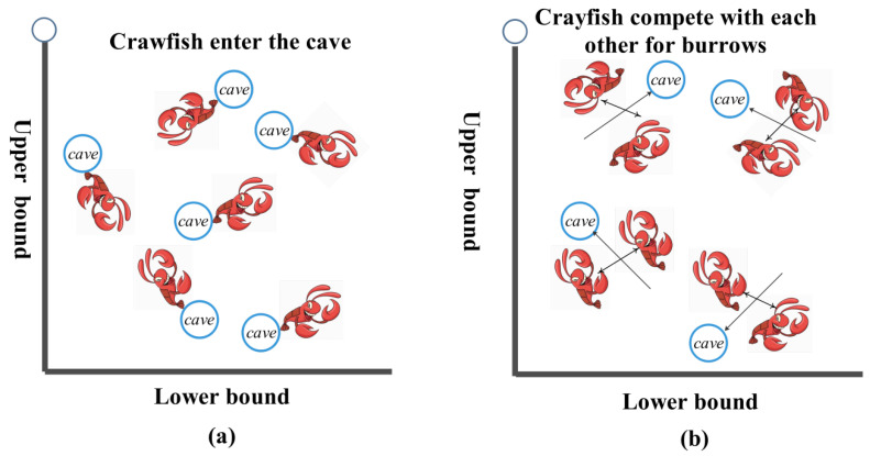 Figure 2
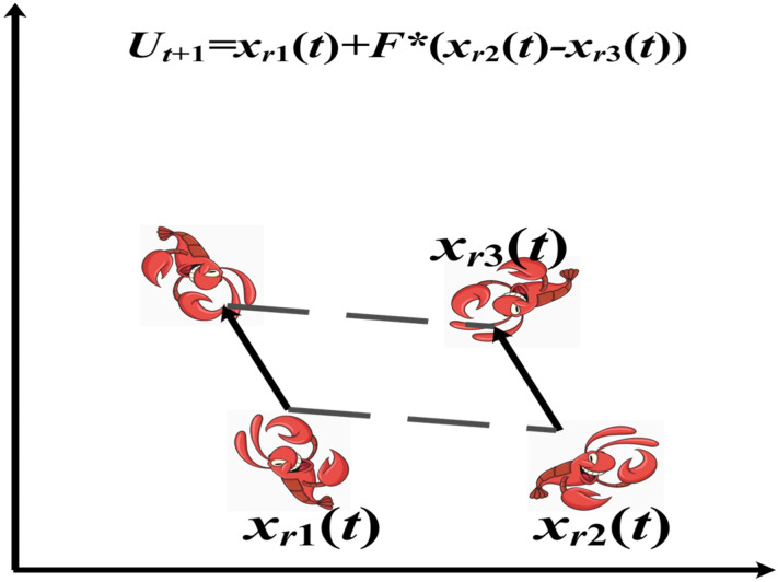 Figure 3
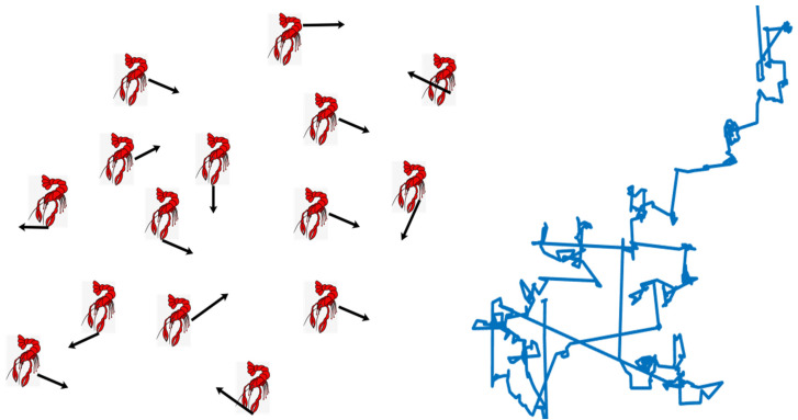 Figure 4
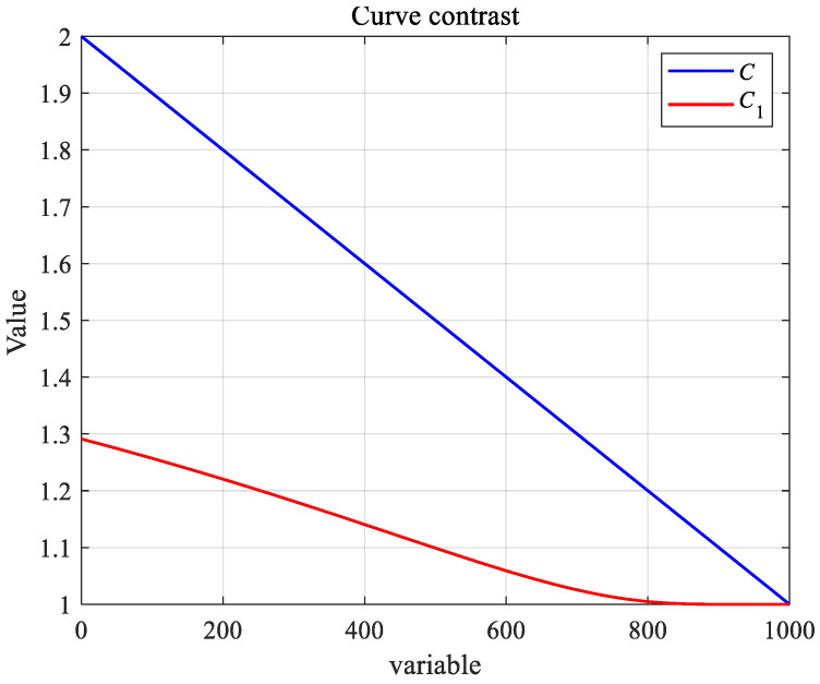 Figure 5
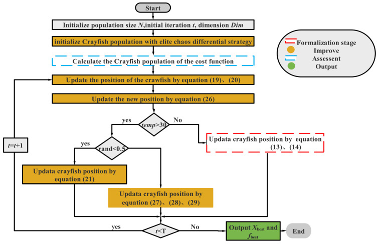 Figure 6
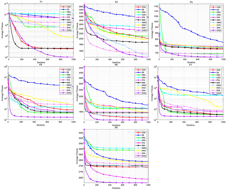 Figure 7
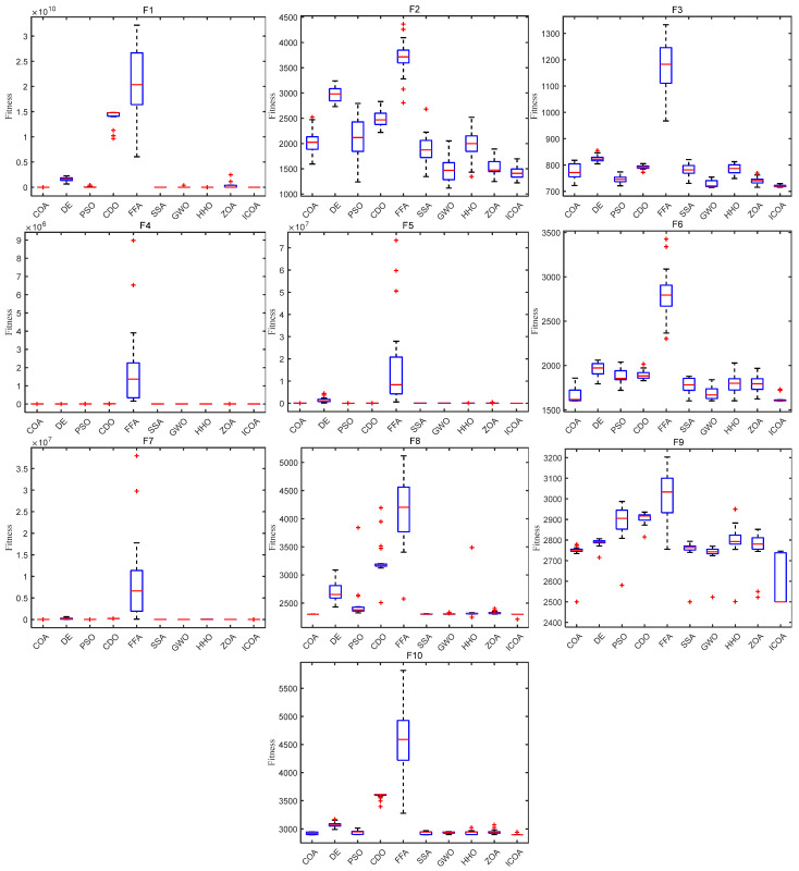 Figure 8
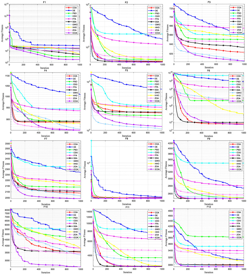 Figure 9
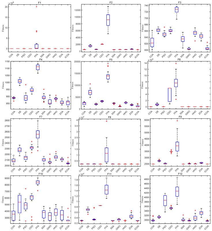 Figure 10
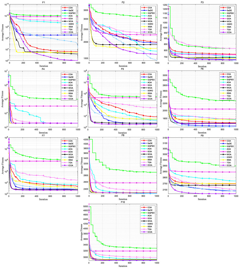 Figure 11
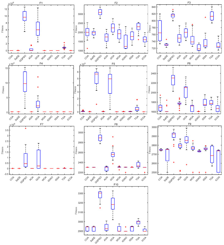 Figure 12
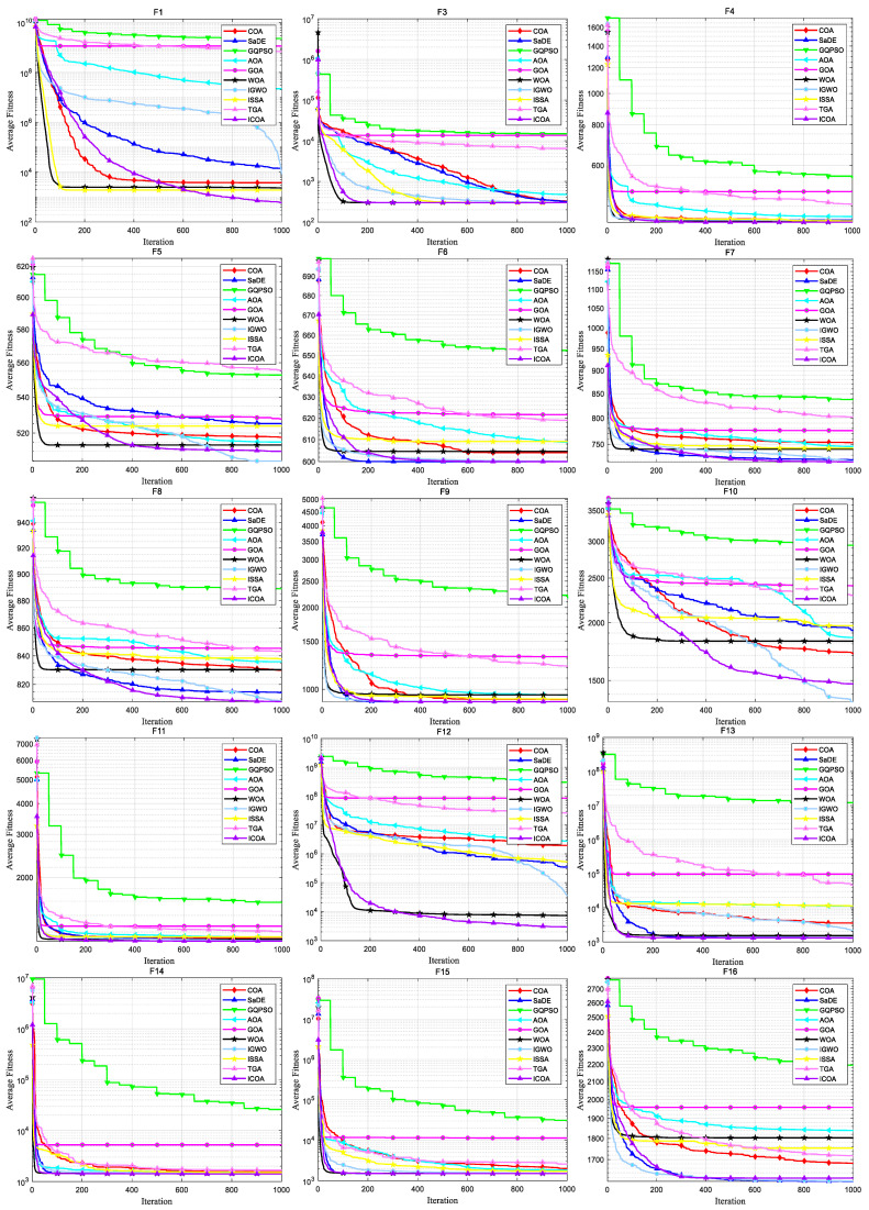 Figure 13
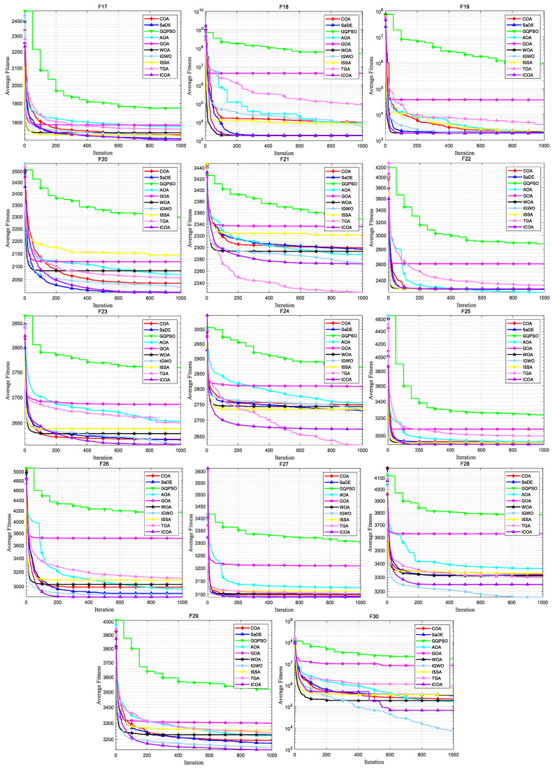 Figure 14
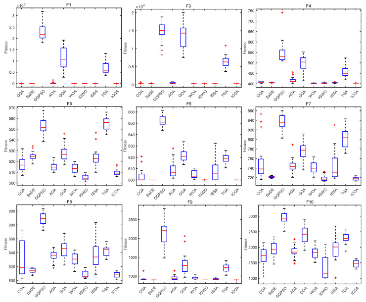 Figure 15
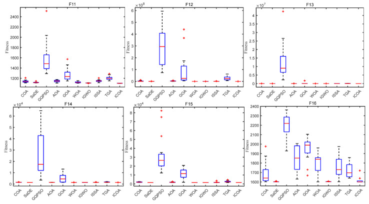 Figure 16
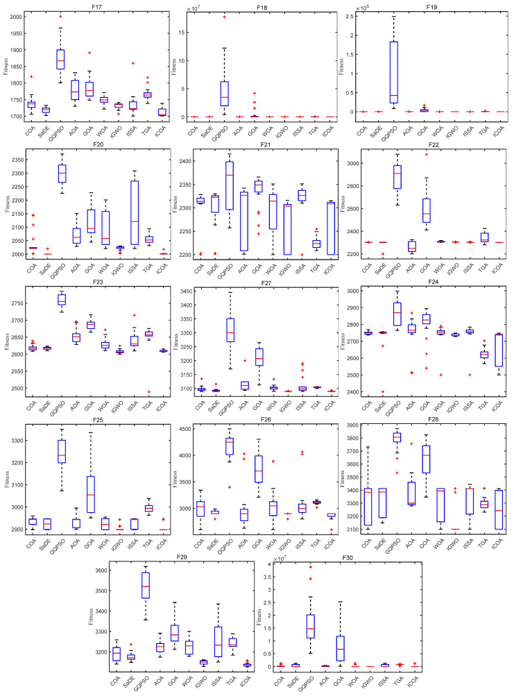 Figure 17
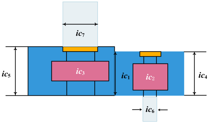 Figure 18
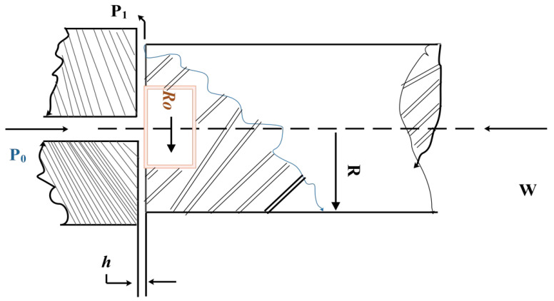 Figure 19
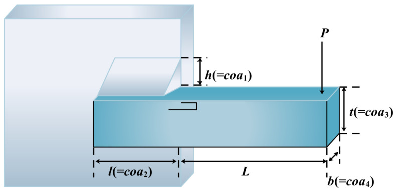 Figure 20
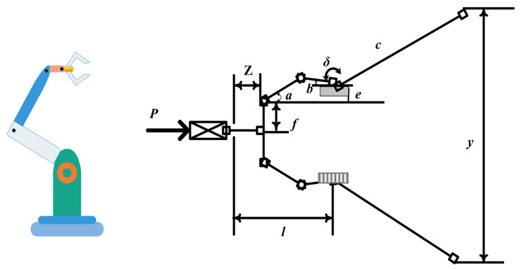 Figure 21
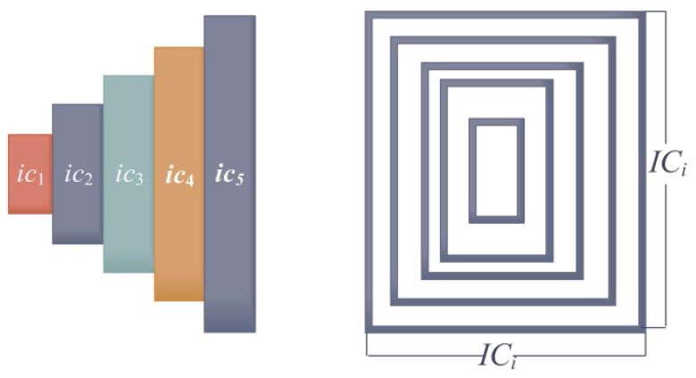 Figure 22
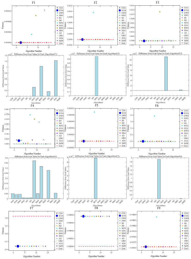 Figure 23
 Figure 24
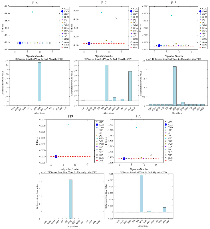 Figure 25
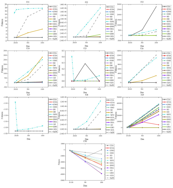 Figure 26
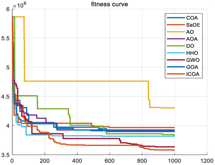 Figure 27
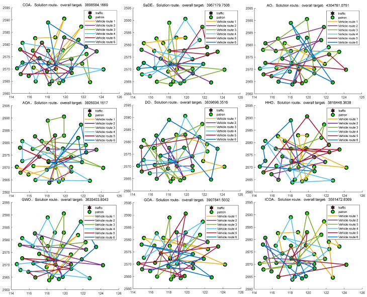 Figure 28
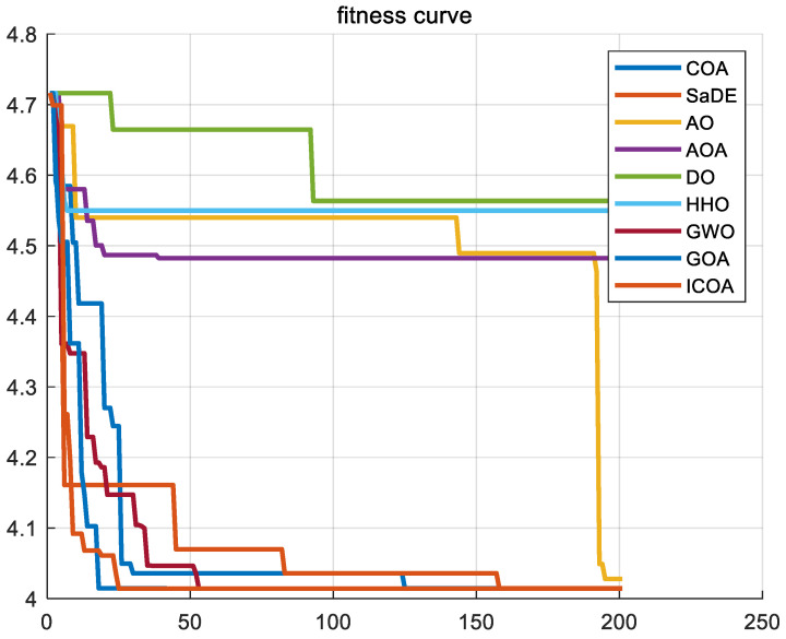 Figure 29
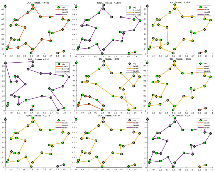 Figure 30
- —Key Research Projects of the Shaanxi Provincial Government Research Office in 2024
- —2024 Shaanxi Provincial Communist Youth League and Youth Work Research Project
Peer Reviews
No public reviews on file for this paper yet. If you reviewed it on a platform where reviews are public (OpenReview, ICLR, NeurIPS, ICML), you can paste yours below so the community can read it here.
Videos
No videos yet. Explain this paper in a talk, walkthrough, or lecture? Add one.
Taxonomy
TopicsMetaheuristic Optimization Algorithms Research
1. Introduction
In recent years, optimization techniques have been increasingly employed to tackle complex problems in various disciplines, including science, engineering, and other relevant fields [1,2,3]. The dimensions and sophistication of these optimization problems have grown exponentially [4]. The traditional gradient descent method and Newton method have been proved to be insufficient to meet evolving engineering needs, and still have many defects in dealing with multi-extremum problems. Therefore, a meta-heuristic algorithm with many advantages, such as randomness, flexibility, ease of implementation, and no need for gradient information [5], comes into being. When it comes to optimizing a given problem, meta-heuristic algorithms can strike a balance between designing efficiently from a local optimum to converging at a point. As a result, they increase the likelihood of finding a global optimum. Meta-heuristic algorithms are extensively utilized, owing to their capacity to efficiently determine the global optimum solution for various optimization problems. These algorithms exhibit several desirable features, including independence from initial conditions and solution domains, robustness, and other exceptional qualities [6,7]. Its practical utility has also been evidenced and employed in various fields, including the multiple traveling salesman problem [8], multilevel threshold image segmentation [9], ship routing and scheduling problems [10], feature selection [11], and multilevel image segmentation [12]. Currently, there are four broad categories.
Group intelligence algorithms are inspired by the effects of animal behavior. Take the PSO [13] algorithm for instance, which draws inspiration from the foraging behavior of birds. In this algorithm, the search space is represented by a collection of particles, each of which embodies a potential solution. To improve efficiency, every particle explores both local and global optima during the search process, aiming to achieve enhanced outcomes. Finally, the velocity and weights of the particles are added to obtain the solution. The Artificial Bee Colony Algorithm (ABC) [14], Ant Colony Optimization (ACO) [15], and Cuckoo Search Optimization (CSO) [16] are the classical algorithms proposed after the PSO algorithm. In recent years, there has been a surge of novel algorithms introduced as a result of extensive research. Consider, for instance, the Snake Optimizer (SO) [17], which finds inspiration from the feeding and reproduction behaviors of snakes. Similarly, the White Shark Optimizer (WSO) [18] draws inspiration from the distinctive navigation and foraging characteristics of white sharks. Alongside these, we also have the Harris Hawk Optimizer (HHO) [19], Artificial Rabbit Optimization (ARO) [20], and Artificial Hummingbird Optimization Algorithm (AHA) [21], and various other algorithms with diverse inspirations and applications.
Algorithms that draw inspiration from various physical phenomena are known as physics-based algorithms. Most famously, Rashedi et al. proposed a physics-based gravitational search algorithm (GSA) [22]. Another renowned physics-based algorithm is the Simulated Annealing Algorithm (SA) [23], which emulates the annealing process of solid matter in the field of physics. These notable examples highlight the application of principles from physics to optimize algorithm design. Evolutionary algorithms are meta-heuristic algorithms that mimic natural evolutionary mechanisms. A prominent example of a physics-based algorithm is the Genetic Algorithm (GA) [24], which simulates the process of biological evolution through natural selection and the hereditary mechanism described in Darwin’s theory. GA uses binary encoding to facilitate interbreeding and mutation in a population of organisms, with each individual representing a candidate solution. Additionally, several new evolutionary algorithms have emerged, including Evolutionary Programming (EP) [25], Differential Evolution (DE) [26], and the Virulence Optimization Algorithm (VOA) [27]. These algorithms draw inspiration from biological and evolutionary principles to optimize their design.
Meta-heuristic algorithms that draw inspiration from human behavioral habits are categorized as human-inspired algorithms [28]. One prominent example in this category is the Harmony Search (HS) algorithm [29]. Other algorithms that share similar principles include Teaching–Learning-Based Optimization (TLBO) [30], Social Group Optimization (SGO) [31], the Group Teaching Optimization Algorithm (GTOA) [32], the Brain Storming Optimization Algorithm (BSO) [33], and the Imperialist Competition Algorithm (ICA) [34]. These algorithms leverage human behavioral patterns to optimize their problem-solving approaches.
In summary, by comparing different features and advantages of meta-heuristic algorithms, the following conclusions can be drawn:
- They are usually inspired by some natural law or mathematical theory [35].
- No theoretical derivation is required to transform the problem into a model that is less dependent on mathematical conditions [36].
- The complexity of the algorithm determines its search rate for finding approximate and suitable solutions [37].
There are two main ways to solve the problem in the meta-heuristic algorithm: (1) a single solution; and (2) A total-based solution. A single-solution-based algorithm that starts its process with a candidate solution and improves on it during iteration. A population-based meta-heuristic algorithm initializes the random solution so that the population tends to the most promising region. Compared to algorithms based on a single solution, population-based meta-heuristics have two advantages: exploration and exploitation [38,39]. The two progress each other, making the algorithm converge faster and improving the global search capability.
According to the No Free Lunch Theory (NFL) [40], there is no perfect algorithm, and there must be a disadvantage to this in some aspect. Based on crawfish’s foraging behavior and summer resort behavior, scholars proposed a new meta-heuristic optimization algorithm, namely the Crawfish Optimization Algorithm (COA) [41]. The COA is a novel way to model the foraging, summer resort, and competitive behaviors of crayfish. By adjusting the temperature, the exploration and development ability of the algorithm are balanced. This algorithm focuses on modeling crayfish behavior and balancing the algorithm by adjusting the temperature. Through a comparative analysis of experimental results, it is observed that the COA demonstrates favorable optimization performance in CEC2014 benchmark functions, as well as in 23 standard benchmark functions and engineering application problems.
However, the COA has its limitations, for instance, low population diversity, poor convergence speed, and low global accuracy of solutions. To address these limitations and improve its optimization capabilities, the paper proposes an enhanced version of the algorithm called the ICOA. The proposed approach includes several improvements. Firstly, an elite chaotic difference strategy is introduced in the initialization stage to promote a more even distribution of crayfish and to obtain an initial population of higher quality. Additionally, to augment the population’s diversity and quality, a differential evolution strategy is integrated before the summer vacation. Moreover, during crayfish summer resort behavior, a Levy flight strategy is employed to amplify their search capability, broaden their exploration range, and enhance their capacity to evade local optima. Finally, an adaptive strategy is introduced during the competition phase to bolster the crayfish’s global search capability, resulting in enhanced solution accuracy and faster convergence in successive iterations.
The efficacy and high competitiveness of the proposed ICOA is demonstrated through comprehensive experimentation on diverse problem sets. Specifically, we evaluate the performance of the ICOA on the CEC2017, CEC2020, and CEC2022 test sets, six engineering applications, 30 high- and low-dimensional constrained problems, and two NP problems. In addition, we evaluated its ability to solve hypersonic missile trajectory planning problems. To assess the effectiveness of the ICOA, a comprehensive comparison is conducted between its solutions and those generated by classical and advanced optimization algorithms. The results obtained were rigorously evaluated by statistical analysis using Wilcoxon rank sum tests to ensure that any significant differences were identified. The key contributions of this research can be summarized as follows:
- (i)The ICOA is proposed by incorporating four strategies, namely, the elite chaotic differential strategy, differential variation strategy, Levy flight strategy, dimensional variation strategy, and adaptive parameter strategy.
- (ii)The effectiveness and potential of the ICOA in addressing complex optimization problems are validated through experimental results obtained from benchmark test sets such as CEC2017, CEC2019, and CEC2020. These results are compared with other state-of-the-art swarm intelligence optimization algorithms, revealing the superior performance of the ICOA. This comparative analysis highlights the algorithm’s effectiveness and reinforces its capability to tackle challenging optimization problems.
- (iii)The ICOA is applied to various real-world industrial design problems, including six specific cases. In addition, thirty high–low-dimension constraint problems, two NP problems, and one hypersonic missile trajectory planning problem are evaluated. The performance of the ICOA is methodically compared to that of classical or state-of-the-art optimization algorithms, providing insights into its efficacy and applicability across diverse problem domains.
The following section of this study will be structured as outlined: Section 2 introduces the inspiration and mathematical model of COA. Section 3 proposes the ICOA, introduces the elite chaotic difference strategy, the difference variance strategy, and the Levy flight strategy, as well as the dimensional variation strategy and the adaptive parameter strategy, and analyzes the algorithmic complexity of ICOA. In Section 4, we conduct numerical experiments and analyze the results of ICOA in comparison to other optimization algorithms using the CEC2017, CEC2020, and CEC2022 test sets. In Section 5, the proposed ICOA is used to solve 6 practical industrial design problems, 30 high–low-dimension constraint problems and two NP problems. In Section 6, a reasonable discussion is presented on the work of this paper. Finally, in Section 7, this paper provides concluding remarks and suggestions for future research directions.
2. Overview of the Crawfish Optimization Algorithm
In 2023, Heming Jia et al. [41] introduced the Crayfish Optimization Algorithm (COA), drawing inspiration from crayfish foraging, summer vacation, and competitive behaviors. The algorithm simulates scenarios where crayfish are on summer vacation, competing, or foraging, and identifies the best location based on varying temperatures. Figure 1 is a schematic diagram of crayfish derived from the literature [41].
The COA is initialized as shown in Equation (1):
where AX is the initial population position, N is the number of populations, dim is the number of population dimensions, is the position of individual i in dimension j, and the value is obtained from Equation (2).
where denotes the lower bound of the j-th dimension, denotes the upper bound of the j-th dimension, and r denotes a random number.
Changes in temperature affect the behavior of crayfish at different stages, which are defined by Equation (3).
where t denotes the ambient temperature and r is a random number.
where µ is the temperature most suitable for crayfish, p is the foraging intake, and σ and C1 are used to control the intake of crayfish at different temperatures.
2.1. Summer Vacation
When the temperature reaches a critical point, the crayfish will go into their burrows and start vacationing. The burrows are ventilated as follows:
where AX_g_ denotes the final optimal position and AX_l_ denotes the current optimal position.
When rand < 0.5, the crayfish will avoid the heat by Equation (6), as shown in Figure 2a.
where t is the current iteration number, t + 1 then indicates the next iteration, and C2 is the decreasing curve, as shown in Equation (7).
where T is the maximum value of the number of iterations.
2.2. Competition Stage
As shown in Figure 2b, when the t > 30C and r ≥ 0.5, crayfish behave according to Equation (8) for burrowing competition.
where t is the temperature and r is the random probability. Z is a random individual, as defined in Equation (9).
2.3. Formalization Stage
When the temperature is 30 °C, this is the right time for crayfish to forage for food. At this point, the food position AX**food is as in Equation (10):
The size of the food, denoted as AQ, is defined as follows:
where C3 is defined as the largest food item with a constant value of 3, is the fitness value of the i-th individual, and is the fitness value at the time of foraging for food.
When AQ > (C3 + 1)/2, crayfish forage for food through Equation (12).
When the food item is small, foraging at this time is shown in Equation (13).
When Q ≤ (C3 + 1)/2, crayfish feed as shown in Equation (14).
At this point, the crayfish has completed all of its behavioral manifestations, that is, it has completed the theoretical process of the COA.
Algorithm 1 is given as pseudo-code for the COA. Algorithm 1: Crayfish optimization algorithmBegin Step 1: Initialization. Set the parameters of the crayfish population. Step 2: Fitness calculation. By calculating the fitness value of the initialized population to get . Step 3: while termination criteria are not met do Defining temperature temp by Equation (3) if temp > 30 do Define cave according by Equation (5) if rand < 0.5 do Crayfish conducts the summer resort stage according to equation (6) else Crayfish compete for caves through Equation (8) end else P and Q can be found by Equation (4) and Equation (11), respectively. if Q ≥ 2 do Crayfish shreds food by Equation (12) Crayfish foraging according to Equation (13) else Crayfish foraging according to Equation (14) end end Update fitness value and output . end while
3. Improved Crayfish Optimization Algorithm with Mixed Strategies
Although the COA has advantages, such as strong optimization ability and fast convergence speed, it is inevitable that it is prone to fall into the local optimum, resulting in low calculation accuracy and affecting optimization ability. In order to further improve the performance of the COA, this section combines the following four strategies to improve the COA and propose the ICOA.
3.1. Elite Chaos Difference Strategies
Chaotic mapping is a stochastic method in nonlinear dynamical systems [42] that initializes populations by using chaotic variables instead of random variables [43]. Therefore, it can perform a thorough search of the solution space more efficiently than a random search that relies primarily on probability [44]. Therefore, this paper considers a well-known type of chaotic mapping: logistic chaotic mapping.
The initial population is considered to be divided into three parts, which are as follows:
- (1)Elite learning selects the population according to a certain ratio as the first part of the initialization decomposition.
where N denotes the number of populations, refers to the i-th crayfish, UB and LB are the upper and lower bounds of the d-th dimension of the population, and e is the elite probability, which is taken as 0.1 in this paper.
(2)Logistic chaotic mapping is carried out on the remaining population according to the ratio column as the second part of the initialization solution.
where ub and lb are the upper and lower bounds of the d-th dimension of the population, [0,1]. In this paper, μ = 3.9, x = 0.5, and x_t_+1 is denoted as the newly generated chaotic mapping values, and is the second part of the candidate solution.
(3)Differential learning, which is performed on the remaining populations, randomizes the elite populations as well as the chaotically mapped populations to be updated by the differential operation to obtain the final differential population, which is the last part of the initial solution.
where t_j_ is some solution of the chaotic mapping population, ub and lb are the upper and lower bounds of the d-th dimension of the population, EX**j is some candidate solution of the elite learning population, and t_j_+1 denotes the new solution after differentiation, and is the last part of the initialization.
The candidate solutions of the above three components are the final initialized crayfish population, expressed as Equation (18).
Performing elite chaotic difference initialization prior to crayfish summer vacation improves the quality of the initial population, allowing for faster access to higher-quality solutions.
3.2. Differential Variation Strategy
By employing the differential mutation strategy, the algorithm effectively enhances the quality of the population. This strategy plays a crucial role in expanding the search range of the population, preventing it from getting trapped in local optima. As a result, the search ability of the algorithm is significantly improved. Therefore, this section considers two operations of differential evolutionary algorithms: the variation operation and the selection operation.
(1)Mutation operation
To determine the mutated individual, we calculate the vector difference between two randomly chosen individuals from the population, following a scaling process. We also consider the vector synthesis of the individual that is being mutated. This approach ensures a diverse set of genetic information is incorporated into the mutated individual. The mathematical representation for the mutation operation is as follows:
where the scaling factor and denotes the ri-th individual in the t-th generation population.
(2)Selection operation
After the mutation operation is completed, Levy flight operation is performed on the mutant individual . The greedy choice is made between the subsequent individual and the original target individual , and the individual with good fitness value is selected to enter the next iteration. The greedy choice model is as follows:
By introducing the differential evolution strategy before the crayfish summer vacation, it is beneficial to consider other individuals in this iteration to update the population information of the current iteration, effectively avoiding the situation where the previous solution is a local optimal solution. It also ensures that better individuals will be generated after the initialization of crayfish individuals and randomly learn from the previous generation of individuals, which increases the diversity of the population, expands the search range of the population, effectively avoids premature stagnation of the algorithm, and enhances its ability to jump out of the local optimum. Figure 3 shows the crayfish undergoing the mutation operation.
3.3. Levy Flight Strategy
Levy flight refers to the use of Levy flight distribution to simulate the random process of flight paths [45,46], which can describe complex random motion trajectories and phenomena with remote correlation and multi-scale properties. The crawfish burrowing process based on this strategy is shown in Equation (21).
where X**new is the new position obtained after the Levy-based flight, X**i is the i-th crayfish, Xf is the cave that the crayfish is going to, is the step scaling factor, which is generally taken as 0.01, and is the Levy randomized path defined as shown in Equation (22), and is the dot product operation.
For ease of computation, define the random numbers as follows,
where u obeys a Gaussian distribution, v obeys a normal distribution in Equation (24). σ is defined as Equation (25), and Γ(x) is a gamma function with β taking the value of 1.5. Figure 4 shows a plot of the simulated trajectory of the Levy flight.
The Levy flight strategy greatly expanded the range of the crayfish’s search when they explored their burrows during the summer vacation, increasing the variety of the search process. The search ability of the algorithm is improved, and the ability to jump out of the local optimal is enhanced.
3.4. Dimensional Variation and Adaptive Parameter Strategy
3.4.1. Dimensional Variation Strategy
For the new population generated after the differential evolution strategy, the t-distribution variational operator is introduced to perturb the optimal individual position [47]. The freedom parameters of the t-distribution variational operator vary with the number of iterations, and the dimensionally variational strategy is specifically defined as follows: assuming dimension equals d and the current optimal solution , then the new solution, obtained by mutating the current optimal solution dimension by dimension, is computed as follows:
where t is the current number of iterations, is the t-distribution with a parameter t of degrees of freedom, and is the random number generated by the t-distribution in the d-th dimension. Since it is impossible to directly judge whether the new position obtained after mutation is better than the original position, this paper uses the principle of greed to judge whether to accept the new position instead of the original optimal position. The greedy principle is used to guide the population to better evolve to the optimal individual position and improve the convergence speed of the algorithm.
3.4.2. Adaptive Parameter Strategy
Inspired by the crayfish entering the burrow during summer vacation, a variable C1 is set to control the crayfish competition for the burrow, and the decreasing curve C is transformed and applied to the competition phase. For the two random individuals X**i and X**j in the competition stage, vector difference is carried out through Equation (27), and adaptive parameter changes are carried out, and then the original XF**j is added to finally obtain the new position XN**i,j.
where C represents the adaptive parameter, F is set to 0.4, and t and T represent the current and maximum number of iterations, respectively.
The adaptive parameter strategy greatly improves the global search capability of the algorithm during the crayfish competition phase and drastically improves the convergence ability of the algorithm. Figure 5 shows the variation in the C and C1 curves.
3.5. ICOA Pseudo-Code
Algorithm 2 gives the pseudo-code of the ICOA, and the flowchart is shown in Figure 6. Algorithm 2: The proposed ICOABegin Step1: Initialization. Crayfish populations were initialized using the elite chaos differential strategy (i.e., Equation (18)). Step2: Fitness calculation. By calculating the population fitness value fitness, the optimal fitness value as well as the corresponding individuals were recorded; Step3: While (t < T) do Defining temperature temp by Equation (3) for i = 1 to N do //Mutation operation //Select operation end for //Dimensional variation for i = 1 to N do if temp > 30 do //Summer resort stage and competition stage if rand < 0.5 do Else //Competition stage For j = 1 to Dim do end for end else //forging stage if P >2 do else end end for Calculate and rank the fitness values. Update t = t+1 Step4: Return. Return the optimum position and fitness value of CrayfishEnd
3.6. Time Complexity of the ICOA
The time complexity of ICOA is commonly dependent on the population size N, the dimension D, the objective function value f for each iteration, and the maximum number of iterations T. The time complexity of ICOA is calculated based on these factors, as shown in Equation (30), Figure 6 shows the flowchart of the ICOA.
Since the parameter T is generally set very large, the simplified Equation is as follows (31):
4. Numerical Experiment and Analysis
In this section, a set of test functions is employed to assess and analyze the performance of the ICOA. The CEC 2017, CEC 2020, and CEC 2022 test sets, consisting of 29, 10, and 12 test functions, respectively, are used to compare the results of the ICOA with those of other classical or recent optimization algorithms. The population size for all algorithms is 50, while the dimension is set at 10 with a maximum number of iterations of 1000. To minimize the influence of randomness on the algorithms, each algorithm is executed independently for 20 trials on the test functions, and the outcomes are compared among the primary algorithm sets.
4.1. ICOA Is Compared with the First Group of Optimization Algorithms
4.1.1. Comparison of the Test Set CEC 2020
In this section, a comparative analysis will be conducted between the proposed ICOA and nine other intelligent optimization algorithms. The selected algorithms can be categorized into three groups: (1) classical intelligent optimization algorithms such as the PSO [14] and the DE [27]. (2) Newly proposed intelligent optimization algorithms in the last year include the Fox for Auricular Fox Algorithm (FFA) [48], the Chernobyl Disaster Optimizer (CDO) [49], and the original Crayfish Optimization Algorithm (COA) [41]. (3) Representative intelligent optimization algorithms in recent years include the Gray Wolf Optimization Algorithm (GWO) [50], HHO [20], the Zebra Optimization Algorithm (ZOA) [51], and the Sparrow Optimization Algorithm (SSA) [52]. Table 1 provides the initial parameters of all optimization algorithms.
Table 2 presents the findings from 20 separate runs of the ICOA compared to other algorithms on the 10-dimensional CEC 2020 test set. The results include the mean, standard deviation, and p-value obtained from the Wilcoxon rank sum test. The ICOA serves as the benchmark, and the statistical outcomes are reported based on 20 runs at a 95% confidence level ( ). In this case, “+” means that the ICOA performs significantly poorly compared to other algorithms, “=” means that there is no significant difference between the ICOA and the algorithm being compared, and “−” and “+” mean the opposite. The bolded data represent the optimal average values and minimum variances of the nine algorithms on each test function.
According to the results shown in Table 2, the ICOA performs best in all ten tested functions. Its optimization ability proves to be better than the original COA in all cases. This indicates that the four strategies in the original COA positively affect the ICOA by improving its convergence speed and computational accuracy. As far as the test function F1 is concerned, the worst value, the mean value, and the standard deviation of the ICOA are significantly smaller compared to other optimization algorithms. These values are also very close to the optimal values. In addition, based on the average ranking, it can be concluded that the ICOA is ranked first (rank = 1). The last row of Table 2 shows the results of the Wilcoxon rank sum test and the ranking of the algorithms. It can be seen that the results of the COA, DE, PSO, CDO, FFA, SSA, HHO, and ZOA are 0/0/10, while the results of the GWO are 0/3/7. The comprehensive analysis shows that the ICOA outperforms the other comparative algorithms on the CEC 2020 test set, and it has a strong competitive advantage.
Figure 7 shows the convergence curve of each algorithm on the CEC 2020 test set. It can be intuitively seen that the COA falls into local optimality on F1, F2, F3, F5, F7, and F9, leading to premature convergence, while the ICOA’s convergence speed and accuracy are greatly improved compared with the COA. And most of the test functions do not stop in the later iteration stage, but continue converging. Comparing the convergence curves of other algorithms, we can see that the ICOA has faster convergence speed and higher convergence accuracy. Especially in F5, F6, F7, F10, the ICOA’s advantage is more obvious.
Figure 8 shows the box diagram of each algorithm on the CEC 2020 test function. It can be seen that on most test functions, the ICOA has a narrow box type, low position, and small median, which indicates that the solution obtained by the ICOA has high consistency and high precision. In addition, the ICOA has fewer outliers on the 10 test functions, which indicates that the algorithm is less affected by the randomness of the strategy during operation. It can be seen from the box diagram that the ICOA is superior to other comparison algorithms in terms of stability and accuracy.
4.1.2. Comparison on Test Set CEC 2022
In order to better verify the performance of the proposed ICOA, a new test set from 2022 was selected for testing. The experiment sets the population size N of all algorithms as 50, the dimension dim as 20, and the maximum number of iterations T as 1000.
Table 3 displays the mean, standard deviation, and Wilcoxon rank sum test p-values for the ICOA and other optimization algorithms based on 20 independent runs on the CEC 2022 test set. The bolded data represent the optimal average values and minimum variances of each test function. As can be seen from Table 3, the optimization ability of the ICOA on 12 test functions has been significantly improved compared with that of the ICOA. On the test functions F1, F2, F6, F7, F8, F9, and F10, the ICOA achieved the best fitness value while also having a relatively small variance. From the last row of Table 3, the Wilcoxon rank sum test statistics results and the rankings of each algorithm are combined to obtain the Wilcoxon rank sum test results of the nine optimization algorithms as follows: 0/0/12, 0/0/12, 0/0/12, 0/0/12, 0/0/12, 1/0/11, 1/1/10, 0/0/12, and 0/1/11. It can be seen that the ICOA outperforms the COA on all the test functions. In general, the ICOA effectively improves the performance of the original algorithm and shows strong ability in solving the CEC 2022 test set. In addition, in Table 3, rank refers to the ranking of each algorithm for each test function based on the size of the average, mean rank refers to the average ranking of the 12 functions, and result is the final algorithm ranking on the CEC 2022 test function. ICOA ranked first place in 10 functions, mean rank, and result in the comprehensive comparison of the algorithms. This shows that the ICOA has better performance not only on most of the proposed test functions, but also on the whole CEC 2022 test set. In conclusion, the ICOA greatly improves the performance of the original algorithm and demonstrates significant potential in solving the CEC 2022 test set.
To further demonstrate the performance of the proposed ICOA, we chose to use Student’s parametric test (t-test) [53,54] for statistical evaluation. T-p in Table 3 is the p-value of the t-test, and the statistical results are given by running the ICOA 20 times at the 95% significance level (t = 0.05), and the experimental results show that ICOA is significant for the original COA on 83.3% of the test functions (10 out of 12 test functions). The other eight comparison algorithms are 100%, 58.3%, 100%, 100%, 100%, 91.7%, 58.3%, 100%, and 91.7%. It can be seen that the ICOA is more than 90% significant for all the other algorithms, and only two algorithms are significant at 58.3% on the CEC 2022 test set. In conclusion, the ICOA improves the performance of the original algorithm in all aspects.
Figure 9 and Figure 10 show the convergence plot and box plot for the 12 test functions, respectively. As can be seen from Figure 9,the ICOA has a faster convergence speed and higher accuracy on test functions F1, F3, F7, and F10, and converges in the later period. On the test functions F2, F4, F6, F9, F11, and F12, although the convergence speed of the ICOA is not very fast, it is obviously superior to other comparison algorithms in the most accurate calculation. In general, when solving CEC 2022 test functions, the ICOA performs well on 90% of the test functions, and is superior to other comparison algorithms in terms of calculation accuracy and convergence speed. Refer to Figure 10. It can be observed that the abnormal points generated by the ICOA are relatively few. In most of the test functions, the median value of the ICOA is superior. Moreover, on the F3, F5, F7, F11, and F12 test functions, the box area is relatively narrow and the position is lower. In general, the ICOA has high stability and good solution accuracy.
4.2. ICOA Compared with the Second Group of Optimization Algorithms
4.2.1. Comparison on CEC 2020 Test Set
In order to further validate the performance of the proposed ICOA, a comparative analysis is conducted with nine other intelligent optimization algorithms on the CEC 2020 test set. (1) Improved classical algorithms include the Gaussian Quantum Particle Swarm Algorithm (GQPSO) [55] and the Adaptive Differential Evolutionary Algorithm (SaDE) [56]. (2) Newly proposed algorithms in the last two years include the Locust Optimization Algorithm (GOA) [57], the Whale Optimization Algorithm (WOA) [58], the Arithmetic Optimization Algorithm (AOA) [59], and the original crayfish algorithm [41]. (3) Improved high-performance algorithms include the Improved Gray Wolf Optimizer (IGWO) [60] and the Improved Sparrow Optimization Algorithm (ISSA) [61]. (4) The Tree Growth Algorithm (TTA) [62] was cited more than 200 times in 2018. The experiments were set for all algorithms with a population size of 50, a dimension of 10, and a maximum number of iterations of 1000. Table 4 shows the initial parameters of all the optimization algorithms used in this section.
Table 5 shows the worst, best, mean, std, and Wilcoxon rank sum test p-values obtained by the ICOA and the second group of optimization algorithms after 20 independent runs of the CEC 2020 test set, and the bolded data are the optimal mean and minimum variance of each test function. It can be seen from Table 5 that the ICOA’s optimization ability in ten test functions has been greatly improved compared with the COA. On the test functions F1, F4, F5, F7, and F10, the ICOA has the smallest standard deviation difference when it reaches the minimum fitness average. On F3 and F6, IGWO reaches the optimal fitness value and has a small variance. In terms of average rank and ranking, SaDE, ICOA, IGWO, and WOA perform better because their average rank is less than 5. The ICOA is in the top three on nine test functions with an average rank of 1.6, ranking first. Therefore, the performance order of nine algorithms in solving the CEC2020 test function is ICOA > IGWO > SaDE > WOA > ISSA > AOA > COA > WOA > GOA > GQPSO. According to the statistical results of the Wilcoxon rank sum test in the last row of Table 5 and the ranking of each algorithm, the Wilcoxon rank sum test results of ten optimization algorithms can be obtained as follows: 0/0/10, 1/0/9, 0/0/10, 0/0/10, 0/0/10, 0/0/10, 0/1/9, 0/0/10, and 1/0/9, respectively. It can be seen that the ICOA is superior to the COA in 10 test functions. In summary, the ICOA effectively improves the performance of the original algorithm and shows strong ability in solving the CEC 2020 test set.
Figure 11 and Figure 12 show the convergence plot and box plot for the 10 test functions, respectively. As can be seen from Figure 11, on the test functions F4, F5, F7, F8, F9, and F10, the ICOA has a faster convergence speed and higher accuracy, and has been converging in the later stage. When solving CEC 2020 test functions, the ICOA performs well on most test functions, and is superior to other comparison algorithms in calculation accuracy and convergence speed. From Figure 12, it can be seen that the ICOA generates fewer outliers. In most test functions, the median of the ICOA is better, the box area of the F1, F4, F5, F7, and F8 test functions is narrow, and the position is lower. In general, the ICOA has high stability and good solving precision.
4.2.2. Comparison on Test Set CEC 2017
It is more convincing to perform comparison experiments on different test sets, so this section describes comparison experiments on the CEC 2017 test set, and the experiments set the population size of all algorithms to be pop = 50, the number of dimensions to be dim = 10, and the maximum number of iterations to be iterated T = 1000.
Table 6 shows the worst, best, mean, Std, and Wilcoxon rank sum test p-values obtained by the ICOA and other optimization algorithms after 20 independent runs of the CEC 2017 test set, and the bolded data are the optimal mean and minimum variance of each test function. As can be seen from Table 6, compared with the COA, the ICOA’s 29 test functions have been greatly improved. On F1, F4, F7, F8, F9, F11, F12, F13, F14, F18, F19, F20, and F29, the ICOA reached the optimal fitness value and the variance was also small. In F15, F17, and F26, although the minimum variance was not reached, the optimal average value was reached. In terms of average rank and ranking, the IGWO, ICOA, SaDE, and WOA perform better because their average rank is less than 5. The ICOA is in the top three on twenty-eight test functions, in the top two on twenty-five test functions, and in first place on fifteen test functions, with an average rank of 1.655, ranking first. According to the statistical results of Wilcoxon rank sum testing in the last row of Table 6, combined with the ranking of each algorithm, the Wilcoxon rank sum test results of nine optimization algorithms can be obtained as follows: 0/0/29, 0/2/27, 0/0/29, 1/1/27, 0/0/29, 1/2/26, 3/2/24, 0/1/28, and 1/1/27. It can be seen that the ICOA is superior to the COA in 29 test functions. In summary, the ICOA effectively improves the performance of the original algorithm and shows strong ability in solving the CEC 2017 test set.
Figure 13 shows the convergence curve of each algorithm on the CEC2017 test set. It can be visually seen that the COA falls into local optimization and leads to premature convergence on F3, F10, F16, F18, F19, F20, F24, F29, and F30, while the ICOA’s convergence speed and accuracy are greatly improved compared with the COA. And most of the test functions do not stop in the later iteration stage, but continue converging. Comparing the convergence curves of other algorithms, we can see that the ICOA has a faster convergence speed and higher convergence accuracy. Especially in F1, F8, F12, F13, F25, F26, and F29, the ICOA’s advantage is more obvious.
Figure 14 shows the box diagram of each algorithm on the CEC 2017 test function. As can be seen that on most test functions, the ICOA has a narrow box type, low position, and small median, which indicates that the solution obtained by the ICOA has high consistency and high precision. In addition, the ICOA has fewer outliers on 29 test functions, which indicates that the algorithm is less affected by policy randomness during operation. It can be seen from the box diagram that the ICOA is superior to other comparison algorithms in terms of stability and accuracy.
5. ICOA Solves All Kinds of Optimization Problems
5.1. ICOA Solves Engineering Optimization Problems
This section aims to assess the efficiency of the ICOA in solving real-world engineering optimization problems by comparing it with other high-performance algorithms. For the six engineering problems involved, the penalty function is first used to transform these constrained problems into unconstrained problems before comparing them. We set the population size, maximum number of iterations, and number of independent runs for all optimization algorithms to 40, 1000, and 30, respectively. The data in bold in this section are all the relevant optimal values that the algorithm solves for each problem.
5.1.1. Speed Reducer Design Problem
The objective of the problem is to obtain the minimum mass under four design constraints; Figure 15 shows a schematic diagram of this problem, and the mathematical models for these four constraints are as follows:
Set the following:
Minimize
Subject it to
The boundaries are as follows:
Table 7 shows the optimal value and corresponding design variables obtained by the ICOA and other optimization algorithms to solve the reducer design problem. These comparison algorithms are GWO [51], HHO [20], DO [63], WFO [64], GOA, SSA, FFA [49], and AOA. Further, Table 8 gives the statistical results of the design problems of the reducer. It can be seen from the table that the ICOA can obtain an optimal cost of 2996.348165, which indicates that the ICOA can obtain the best result in solving the design problem of the reducer.
5.1.2. Hydrodynamic Thrust Bearing Design Problems
The primary aim of this design problem is to minimize the power loss in the bearings [65]. Figure 16 illustrates this issue. This objective is mathematically expressed as follows:
The min is the following:
Subject to
where
The boundaries are as follows:
Table 9 presents the comparison of the optimal values and design variables achieved through the ICOA, as well as several other optimization algorithms, in addressing the problem of hydrostatic thrust bearing. These algorithms include GWO [51], HHO [20], DO, WFO, GOA, SSA, FFA [49], and AOA [59]. The results of the mathematical calculations for this problem are further given in Table 10. From the table, we can observe that the ICOA achieves an optimal cost of 2996.348165 for this design problem. This result highlights the superiority of the ICOA over other algorithms in obtaining the optimal solution for this specific problem.
5.1.3. Welded Beam Design Problem
The main objective of this specific problem is to formulate a design for a welded beam that minimizes the total cost [66]. Figure 17 is a simulation of this problem. The problem can be mathematically represented as follows:
Minimize
Subject it to:
where
The boundaries are as follows:
As shown in Table 11, the optimal values and the corresponding four design variables solved by the ICOA are compared with the results obtained by COA [41], GWO [51], HHO [20], SO [18], DO [63], WFO [64], GOA, SSA, ISSA, FFA [49], and AOA [59]. The statistical results of each algorithm for solving this problem are given in Table 12. By examining the results, it becomes evident that the ICOA consistently outperforms other algorithms in terms of all metrics, indicating its capability to offer higher-quality and more stable solutions for this problem. This underscores the robust adaptability of the ICOA.
5.1.4. Robot Gripper Design Optimization Problem
This design problem primarily aims to address the range between the maximum and minimum values generated by the clamping arm of the robot [67]. Figure 18 is a simulation of this problem. The problem can be formulated as follows:
Set
Minimize
Subject it to
where
The boundaries are as follows:
Table 13 shows the optimal value and optimal corresponding variable obtained by the ICOA and other optimization algorithms for solving the robot arm design problem. These comparison algorithms are as follows: COA [41], SCA [68], AO [69], BWO [70], DO [63], WFO [64], GOA, SSA, RSA [71], FFA [49], GRO [72], and AOA [59]. Table 14 further gives the statistical results of the robot clamp arm design problems. As can be seen from the table, the ICOA can obtain the optimal cost of 7.2740693811E−17, which is better than COA.
5.1.5. Cantilever Beam Design Issues
The engineering problem at hand is relatively straightforward, aiming to minimize the weight of a cantilever beam by utilizing five variables [73]. Figure 19 is a simulation of this problem.
Minimize
Subject it to
The boundaries are as follows:
As shown in Table 15, the ICOA was used to solve the cantilever beam design problem, and the optimal values and the corresponding four design variables solved by the ICOA were compared with the results obtained by COA [41], SCA, AO, BWO, WFO, GOA, SSA, FFA [49], and AOA [59]. The numerical results of each algorithm solving this problem alone are given in Table 16. By analyzing the results, it becomes apparent that the ICOA consistently produces smaller values for all the indicators. This outcome indicates that the ICOA is capable of providing higher-quality and more stable solutions for this problem. This highlights the strong performance of the ICOA.
5.1.6. Heat Exchanger Design Issues
This design application is taken from Hawk and Hitkowski [74]. It features a linear objective function whose minimization is bounded by six inequalities (three of which are non-convex). All eight variables are bounded. The parameters are slightly modified, and the mathematical model is as follows [74]:
Minimize
Subject it to
The boundaries are as follows:
As shown in Table 17, the ICOA is used to solve heat exchanger design problems. The optimal value of the ICOA solution and the corresponding eight variables were compared with the results obtained by ISSA, GWO [51], AOA [59], AO, COA [41], HHO [20], WFO, GOA, BWO, DO, SO [18], GRO. Table 18 shows the numerical results of each algorithm to solve this problem. It can be seen that the ICOA solves all the indicators relatively quickly. This shows that the ICOA provides more stable and more accurate solutions for heat exchanger design problems.
5.2. ICOA Solves Constrained Optimization Problems
This section involves the utilization of a set of mathematical functions, encompassing a total of 30 functions. To narrow down the scope, 20 functions were specifically examined within the context of small-dimensional problems. Additionally, the remaining 10 functions were explored in relation to large-dimensional problems. Notably, these functions encompass six distinct forms. Each section provides detailed and comprehensive information pertaining to the specific functions under examination. Detailed information on the functions considered is available online at https://www.sfu.ca/~ssurjano/ (accessed on 14 April 2025). In this section, thirteen comparison algorithms are selected from COA [41], AO, AOA [59], DO, HHO [20], GWO, SaDE, SO [18], GRO, ISSA, BWO, WFO [64], and GOA.
5.2.1. Low-Dimensional Problems
In this section, the ICOA and other comparative algorithms are utilized to evaluate 20 benchmark functions with dimensions ranging from 2 to 6 (F1 to F20). Additionally, the summary of the optimal values obtained by each algorithm and the target values of the benchmark functions is presented in Table 19 and Figure 20. The results show that the proposed ICOA outperforms the original algorithm and most of the comparative algorithms in terms of optimization and providing values close to the optimal response of the target.
Table 19 shows that on low-dimensional problems, the ICOA can achieve optimal results on F7F14 and F16F20, which are closer to the required objective values. And on 15 low-dimensional problems, the ICOA solution has better results than the original algorithm solution, thus verifying that the improved crayfish algorithm is more accurate. Figure 20 gives a comparison plot of the optimal fitness values of the ICOA with the other 12 intelligent optimization algorithms on the low-dimensional problem, as well as a histogram of the difference values of each algorithm with respect to the objective value of each function. The comparison chart shows that ICOA works best on F1, F2, F3, F5, F6, and F9~F20. The histogram clearly shows that the ICOA is either the same or closer to the objective value on each function compared to the original algorithm. This shows that the ICOA is more accurate than the original algorithm when dealing with low-dimensional math problems.
5.2.2. Higher Dimensional Problems
In order to evaluate the performance of the algorithms on large-scale problems, 10 benchmark functions (F21 to F30) have been considered. The dimensions studied in this section are 30, 100, 500, and 1000. They were executed 30 times for each problem, algorithm, and dimension. The results show that the proposed algorithm has good performance in estimating the optimal response for large-scale problems. Table 20, Table 21, Table 22, Table 23 and Table 24 provide the results of all the algorithms implemented in this section.
From Table 20, we can see that the ICOA is still suitable for some high-dimensional problems and achieves the best results. Functions F21 to F22 demonstrate cases where the optimal value obtained by the ICOA outperforms the original algorithm, providing evidence that the ICOA is more effective in solving large-scale problems.
Table 21, Table 22 and Table 23 present the optimal solutions obtained by the ICOA, as well as other comparative algorithms, on dimensions of 100, 500, and 1000 for the functions F21 to F30. In particular, it can be seen that for functions F21, F23, F26, and F28, the ICOA produces the best results, while for functions F24, F25, F29, and F30, the ICOA achieves superior optimal values compared to the original algorithm. This underscores the enhanced efficiency and accuracy of the ICOA when solving large-scale problems. Overall, the ICOA offers valuable advantages and increased accuracy in tackling large-scale problem solving.
Figure 21 gives the optimal fitness value plot of the ICOA with other intelligent optimization algorithms on high-dimensional problems, and 30, 100, 500, and 1000 dimensions are chosen to better illustrate the ability of the ICOA to deal with high-dimensional problems. On F21F28, the ICOA achieves optimal results on all four dimensions, which shows that the ICOA has a strong advantage on high-dimensional problems. And on F21F29, the ICOA is better than the original algorithm’s optimization results, which shows that the ICOA is more advantageous in solving high-dimensional problems and has higher accuracy than the original algorithm.
5.3. ICOA Solving the NP-Hard Problem
In this subsection, our goal is to examine the extensibility and adaptability of the ICOA to more challenging problem fields, in general, and, in particular,, mixed-integer affine problems. To evaluate the performance of the ICOA on complex problems, we will utilize it in solving two representative mixed-integer nonlinear problems. By comparing the results with other algorithms known for their good performance, we can ascertain the effectiveness of the ICOA in tackling such challenges. These algorithms are SaDE, AO, GOA, AOA, DO, HHO [20], GWO, and COA [41]. Each problem experiment setup parameter was set according to the problem. In our experimental setup, we have established the number of iterations to be T = 200, alongside a population size of N = 50.
A.NP1. logistics distribution [75]
Logistics distribution has been a significant factor impeding the development of the logistics industry in recent times. Especially for dairy enterprises, cold chain distribution is a very critical link. Coordination and optimization of multiple variables are required in cold storage, transportation, etc., to achieve the purposes of cost reduction and efficiency improvement.
To address this problem, the ICOA is designed for the vehicle optimization of cold chain distribution, which is verified to have the advantages of short solution time, fast convergence, and high solution accuracy by comparing with other algorithms.
Figure 22 gives the convergence plot of the algorithms of the ICOA and other algorithms in finding the shortest path to the ball. The ICOA clearly achieves the best results, indicating that ICOA solves this problem with high accuracy. Figure 23 illustrates that the ICOA achieves optimal vehicle scheduling, minimizing the cost to the organization. It shows that the ICOA is more advantageous in solving the problem of vehicle scheduling optimization.
Table 24 gives the optimal values as well as the mean and variance when the ICOA solves NP1. The bolded data are the optimal values for each metric. Taking a look at Table 24, it is evident that the ICOA performs better than other methods in terms of the optimal value, mean, and variance when solving this problem. This observation supports the notion that the ICOA delivers superior quality and stability when solving the problem at hand, indicating its high accuracy and reliability.
B.NP2. TSP issues [75]
Solving the TSP focuses on determining the shortest path by selecting the smallest distance among all available paths. Therefore, we apply the proposed ICOA to this problem to find the shortest path.
By conducting an analysis of Figure 24 and Figure 25, it becomes evident that the ICOA outperforms other algorithms in successfully solving the traveling salesman problem (TSP). It consistently obtains the optimal solution, namely the shortest path, surpassing the performance of alternative algorithms. This shows that the ICOA has a greater advantage than other algorithms in solving the TSP, thus indicating that the ICOA has a good ability to solve the TSP.
Table 25 shows the optimal value, average value, and variance when the ICOA solves the TSP. The bolded data are the optimal values under each index. Table 25 shows that the ICOA has the lowest optimal value and the lowest average value when solving this problem. The ICOA can give a better solution to solve this problem, which shows that the ICOA has a higher precision.
6. Discussion
Compared with other classical optimization methods, the ICOA has better optimization performance. Based on three test sets, six engineering problems, high- and low-dimensional mathematical problems, and NP problems, combined with a hypersonic missile path planning verification experiment, the implementation of the ICOA is discussed in detail. On the test set CEC 2020, the ICOA ranked first among all eight optimization algorithms, indicating that the addition of four strategies greatly improved the performance of the COA. On the new test set, CEC 2022, the ICOA ranked second in two test functions, but first in the remaining ten test functions, indicating that the proposed ICOA is equally adaptable and effective in the new problem. To test the powerful performance of the ICOA, we re-selected nine additional optimization algorithms and tested a variety of test functions in the CEC2017 test set. The results show that the ICOA ranks first in fourteen test functions and in the top three in twenty-eight test functions, accounting for 95.6% of the top three, with a ranking value of 1.6. This comprehensively demonstrates that the proposed ICOA represents a substantial improvement to the development and exploration capabilities of the original COA. Finally, the proposed ICOA is optimized for both high- and low-dimensional mathematical functions and NP problems. It is proved that the ICOA has great advantages in high-dimensional problems. These tests verify the effectiveness and reliability of the ICOA in engineering optimization.
7. Conclusions and Future Work
The main research focus of this paper is as follows. (1) An improved crayfish algorithm (ICOA) based on the elite chaotic difference strategy, the difference variance strategy, the Levy flight strategy, and the multi-strategy of the dimensional variation strategy and adaptive parameter strategy is proposed. The main purpose of the proposed ICOA is to prevent the premature local convergence of the COA and to solve some problems with low precision, so as to improve the accuracy of the COA and expand the search ability of the COA. (2). Several test sets, engineering examples of different sizes, a set of low- and high-dimensional mathematical functions, two NP problems, and path planning problems were used to verify the performance of the ICOA. This included CEC 2017, CEC 2020, and CEC 2022, and three test sets, as well as six engineering examples, twenty low-dimensional mathematical functions, ten high-dimensional mathematical functions, and, finally, the use of large-scale NP problems, and a hypersonic missile trajectory planning problem.
The following conclusions were obtained using numerical and graphical comparisons of the ICOA with other intelligent optimization algorithms:
- (1)The elite chaotic difference strategy improves good initial solutions for the ICOA, prevents blind searches, and ensures a more uniform distribution of populations in space.
- (2)The ICOA ranks first in all the CEC 2020 test sets, and tenth out of twelve test functions in the CEC 2022 test set, based on the first set of comparison algorithms. Based on the second set of comparison algorithms on the CEC 2017 and CEC 2020 test sets, respectively, the combined rank is first (rank = 1.6, 1.517). It shows that the Levy flight strategy and dimensional variation strategy and adaptive strategies greatly improve the convergence and search ability of the COA.
- (3)The results of six engineering examples and hypersonic factor missile trajectory planning show that the ICOA is more efficient and stable than other algorithms in solving practical engineering problems.
- (4)The outcomes obtained from the evaluation of high-dimensional and low-dimensional mathematical problems, along with complex NP problems, demonstrate that the enhanced strategy significantly enhances the optimization capability of COA. Moreover, it also improves the stability in solving large-scale problems. These results imply that the ICOA outperforms the original algorithm in terms of accuracy and the quality of solutions for large-scale problems.
Moving forward, leveraging the superior abilities of the ICOA in handling diverse complex problems, our future work will focus on optimizing even more complex global optimization problems. To validate the performance of the ICOA further, we plan to tackle real-world engineering problems, thus providing practical evidence of its effectiveness. Furthermore, the proposed ICOA has the potential to address practical problems across diverse fields. For instance, it can handle scheduling tasks in fog computing, complex engineering applications, parameter estimation in photovoltaic modeling [76], multi-threshold image segmentation [77], 3D path planning of UAVs, and many more areas.
The reference list from the paper itself. Each links out to its DOI / PubMed record.
- 1Garip Z. Karayel D. Çimen M.E. A study on path planning optimization of mobile robots based on hybrid algorithm Concurr. Comput. Pract. Exp.202234 e 672110.1002/cpe.6721 · doi ↗
- 2Wansasueb K. Panmanee S. Panagant N. Pholdee N. Bureerat S. Yildiz A.R. Hybridised differential evolution and equilibrium optimiser with learning parameters for mechanical and aircraft wing design Knowl.-Based Syst.202223910795510.1016/j.knosys.2021.107955 · doi ↗
- 3Yuan M. Li Y. Zhang L. Pei F. Research on intelligent workshop resource scheduling method based on improved NSGA-II algorithm Robot. Comput.-Integr. Manuf.20217110214110.1016/j.rcim.2021.102141 · doi ↗
- 4Zhan Z.H. Shi L. Tan K.C. Zhang J. A survey on evolutionary computation for complex continuous optimization Artif. Intell. Rev.2022555911010.1007/s 10462-021-10042-y · doi ↗
- 5Merrikh-Bayat F. The runner-root algorithm: A metaheuristic for solving unimodal and multimodal optimization problems inspired by runners and roots of plants in nature Appl. Soft Comput.20153329230310.1016/j.asoc.2015.04.048 · doi ↗
- 6Mzili T. Rif M.E. Mzili I. Dhiman G. A novel discrete rat swarm optimization (DRSO) algorithm for solving the traveling salesman problem Decis. Mak. Appl. Manag. Eng.2022528729910.31181/dmame 0318062022 m · doi ↗
- 7Jia H. Sun K. Li Y. Cao N. Improved marine predators algorithm for feature selection and SVM optimization KSII Trans. Internet Inf. Syst. (TIIS)20221611281145
- 8Mzili I. Mzili T. Rif M.E. Efcient routing optimization with discrete penguins search algorithm for MTSP Decis Mak. Appl. Manag. Eng.2023673074310.31181/dmame 04092023 m · doi ↗