Recovering the cluster picture of a polynomial over a discretely valued field
Lilybelle Cowland Kellock

TL;DR
This paper shows how to determine the cluster picture of a polynomial over a discretely valued field without knowing its roots.
Contribution
The paper introduces a method to recover the cluster picture using valuations of explicit polynomials in the coefficients.
Findings
Valuations of specific polynomials in the coefficients determine the cluster picture of the polynomial.
This method applies to hyperelliptic curves and determines properties of their minimal models.
The approach generalizes a result from Tate's algorithm for elliptic curves to hyperelliptic curves.
Abstract
For f(x) , a separable polynomial of degree d over a discretely valued field K , we describe how the cluster picture of f(x) over K , in other words, the set of tuples {(ord(xi−xj),i,j):1≤i<j≤d} , where x1,…,xd are the roots of f(x) , can be recovered without knowing the roots of f(x) over K¯ . We construct an explicit list of polynomials gd(1),…,gd(td)∈ℤ[A0,…,Ad−1] such that the valuations ord(gd(i)(a0,…,ad−1)) for i=1,…,td uniquely determine this set of distances for the polynomial f(x)=cf(xd+ad−1xd−1+⋯+a0) , and we describe the process by which they do so. We use this to deduce that if C:y2=f(x) is a hyperelliptic curve over a local field K . This list of valuations of polynomials in the coefficients of f(x) uniquely determines the dual graph of the special fibre of the minimal strict normal crossings model of C/Kunr , the inertia action on the Tate module…
Genes, proteins, chemicals, diseases, species, mutations and cell lines named across the full text — each resolved to its canonical identifier and authoritative record.
Click any figure to enlarge with its caption.
 Figure 1
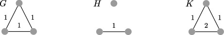 Figure 2
 Figure 3
 Figure 4
 Figure 5
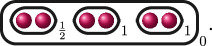 Figure 6
 Figure 7
 Figure 8
 Figure 9
 Figure 10
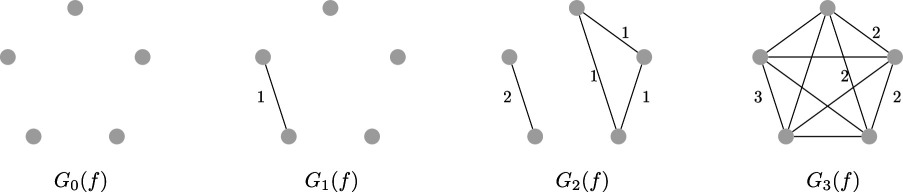 Figure 11
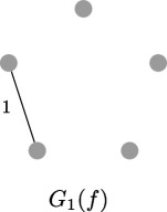 Figure 12
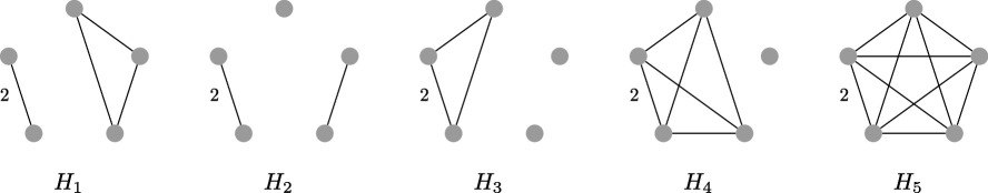 Figure 13
 Figure 14
 Figure 15
 Figure 16
 Figure 17
 Figure 18
 Figure 19
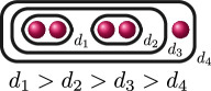 Figure 20
 Figure 21
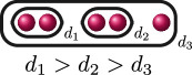 Figure 22
 Figure 23
 Figure 24
 Figure 25
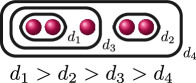 Figure 26
 Figure 27
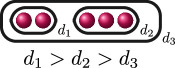 Figure 28
 Figure 29
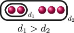 Figure 30
 Figure 31
 Figure 32
 Figure 33
 Figure 34
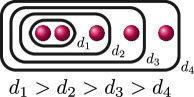 Figure 35
 Figure 36
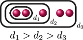 Figure 37
 Figure 38
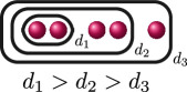 Figure 39
 Figure 40
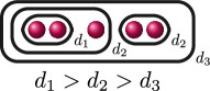 Figure 41
 Figure 42
 Figure 43
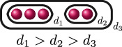 Figure 44
 Figure 45
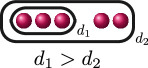 Figure 46
 Figure 47
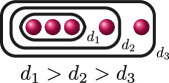 Figure 48
 Figure 49
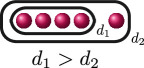 Figure 50
|
valuation of | |||
|---|---|---|---|
|
graph |
rational function |
|
|
|
|
|
|
|
|
|
|
|
|
|
|
a discretely valued field. |
|
|
the valuation with respect to a uniformizer of |
|
|
the algebraic closure of |
|
|
a separable polynomial with coefficients in |
|
|
the discriminant of |
|
|
a weighted graph with vertex set |
|
|
an edge between vertices |
|
|
the depth of the |
|
|
the number of distinct depths in the cluster picture of |
|
|
the number of pairs of roots satisfying ord |
|
|
the |
|
|
the set of auxiliary graphs on |
|
|
the rational function associated with a weighted graph, see definition 1.3. |
|
|
a summand of |
|
|
|
|
|
a summand of |
|
|
the identity element in |
|
|
|
|
|
|
|
|
|
|
|
|
|
|
|
graph name |
auxiliary graph |
summand of |
cluster picture |
depths |
example |
|---|---|---|---|---|---|
|
|
|
|
|
|
|
|
|
|
|
| ||
|
|
|
|
| ||
|
|
|
|
|
| |
|
|
|
|
|
| |
|
|
|
|
|
| |
|
|
|
|
|
| |
|
|
|
|
|
|
|
|
|
|
|
|
|
|
|
|
|
|
| ||
|
|
|
|
|
|
|
|
|
|
|
|
|
|
|
|
|
|
|
|
|
|
|
|
|
|
|
|
|
|
|
|
|
|
|
|
|
|
|
| ||
|
|
|
|
|
| |
|
|
|
|
|
| |
|
|
|
|
|
| |
|
|
|
|
|
|
|
|
|
|
|
| ||
|
|
|
|
|
| |
|
|
|
|
|
| |
|
|
|
|
|
| |
|
|
|
|
|
|
|
- —Engineering and Physical Sciences Research Councilhttp://dx.doi.org/10.13039/501100000266
Peer Reviews
No public reviews on file for this paper yet. If you reviewed it on a platform where reviews are public (OpenReview, ICLR, NeurIPS, ICML), you can paste yours below so the community can read it here.
Videos
No videos yet. Explain this paper in a talk, walkthrough, or lecture? Add one.
Taxonomy
TopicsAlgebraic Geometry and Number Theory · Commutative Algebra and Its Applications · Algebraic structures and combinatorial models
Introduction
Let be a separable polynomial of degree over a discretely valued field . In this paper, we address the question of how the set of tuples up to reordering of the roots of , also known as the cluster picture, can be recovered from valuations of polynomials in the coefficients of . The results of this paper mean that the configuration of the distances between the roots can be recovered without having to find the roots of over , which could be defined over large extensions if is large. The main result we prove is the following theorem, which states that the configuration of the distances between the roots of can be recovered from a finite list of polynomials in the coefficients of , with this list depending only on the degree of . We describe this list explicitly in theorem 1.2. Throughout, we use to denote the valuation with respect to a uniformizer of .
Theorem 1.1 (= theorem 4.3). There exists a finite and explicit list of polynomials for which, if is a separable polynomial of degree over a discretely valued field , for uniquely determines the set of tuples
up to reordering of the roots of .
Knowing the configuration of the distances between the roots of a polynomial over a discretely valued field is of significant importance to the study of elliptic and hyperelliptic curves. For instance, if is an elliptic curve over a local field of residue characteristic , there are two possibilities for the configuration of the roots of the cubic, and this tells us the reduction type of the curve. In some labelling of the roots , and , either
(i) for some , or(ii) and for some with ,
and has potentially good reduction if and only if has root configuration . Further to this, we can read off the Kodaira type of the curve from the root configuration using Tate’s algorithm (see, for example [1], example 1.13). More generally, for a hyperelliptic curve given by a Weierstrass equation over a discretely valued field , extensive work has been undertaken on recovering important arithmetic information such as reduction types from the configuration of the differences of roots, the methodology for which was introduced in [2]. The goal of this paper is to provide a method for recovering the configuration of the differences of roots of a polynomial from polynomials in the coefficients of , thus giving an analogue to a corollary of Tate’s algorithm in the setting of hyperelliptic curves, that for an elliptic curve over a local field of residue characteristic , one can obtain the Kodaira type of from the coefficients of a Weierstrass equation for using the valuation of and . We state the results of this paper pertaining to hyperelliptic curves in §1.1.
In the following theorem, we explicitly describe the polynomials from theorem 1.1 that recover the configuration of the distances between the roots. The polynomials are described using rational functions in the roots of that are associated with weighted graphs on vertices called auxiliary graphs (see definition 1.5). The rational functions in the roots of are defined in terms of differences of roots so that their valuations can be related to the distances between the roots (see §3). They are quotients of polynomials that are symmetric in the roots of so they can be written in terms of the coefficients of , and thus the roots of over do not need to be known a priori in order to evaluate them.
Theorem 1.2 (see theorem 4.1). Let be a separable polynomial of degree over a discretely valued field . The valuations for every (see definitions 1.3 and 1.5) uniquely determine the set of tuples
up to reordering of the roots of .
Theorem 1.2 is a simplified version of theorem 1.8, which explicitly describes how to recover the set of tuples from the valuations.
Definition 1.3. Let be a weighted graph, where . Fix a labelling of the vertices of corresponding to the variables , thus considering as a labelled graph. There is a natural action of on via the action on the vertices. This is given explicitly by letting
where and . Let under this action. We define
To , associate the rational function , where the sum is taken over all . For a separable polynomial with a fixed labelling of the roots , write and for and , respectively, and note that and do not depend on the labelling of the vertices of or the roots of .
Example 1.4. For the complete graph on vertices where each edge has weight , we have , where . In general, the rational functions will all look like a symmetric polynomial in divided by a power of . For example, for the graph on three vertices below its associated rational function is as follows, with .
Definition 1.5. Define to be the set of all weighted graphs on vertices , for which:
(a) for some ;(b) If and all edges of weight are removed, the remaining graph is a disjoint union of complete graphs. Equivalently, allocating the edges not in weight , for , .
We call graphs in auxiliary graphs on vertices.
In example 1.6, we write down two of the rational functions associated with graphs in and use these to demonstrate how the rational functions from theorem 1.2 can be used to recover the configuration of the distances between the roots of a cubic. The methods of this paper generalize the phenomenon outlined in this example to recover more complicated root configurations for higher degree polynomials.
Example 1.6. The graphs in are:
If is an elliptic curve over a discretely valued field, there are two possibilities for the configuration of the roots. In some labelling of the roots , and of , either
(i) for some , or(ii) and for some with .
The following table gives the rational function associated with the graphs with weight in when evaluated on the roots of , and the valuation of these rational functions when evaluated on elliptic curves with root configurations and . We omit since so its valuation does not give us any further information.
**: **
We can use these rational functions and to distinguish between case and , since, using the fact that , the cubic has root configuration if and only if . If we are in case then , and if we are in case then . In case , we have .
Remark 1.7. If we write and from example 1.6 in terms of and , we obtain the result that has root configuration if and only if , which is equivalent to when has residue characteristic . Since root configuration is equivalent to having potentially multiplicative reduction (see, for example [1], example 1.13), we recover the result that has potentially multiplicative reduction if and only if .
In the following theorem, we give a procedure that recovers the cluster picture from the list of rational functions in the roots of associated with the weighted graphs in . For the definition of , , and see definitions 1.9 and 1.10. We explicitly write out the full algorithm for degree polynomials in §5, where we give a table listing the graphs in , their associated rational functions and a description of how the configuration of the distances between the roots can be recovered from these.
Theorem 1.8 (= theorem 4.1). Let be a separable polynomial of degree over a discretely valued field .
(i) Given and , let
and for let
Out of the graphs in , let be the graph with the most edges satisfying . Then
(ii) Given and , where is the complete graph on vertices, fix a labelling of the vertices of . Then there is a labelling of the roots of such that if and only if in . In particular, the set of tuples
up to reordering of the roots , is uniquely determined by and .
Definition 1.9 (see definition 2.4). Let be a separable polynomial over a discretely valued field and let be the roots of in . Define to be the -th largest valuation in the set , and define to be the number of distinct valuations in this set. Define .
Definition 1.10 (see definition 2.4). Let be a separable polynomial over a discretely valued field and fix a labelling of the roots of in . For , define , where
(i) and ;(ii) if for .
We consider as an unlabelled graph and call it the * -th auxiliary graph* associated with . Define to be the empty graph on vertices and , where if for . That is, is the -th auxiliary graph associated with a cluster picture but with added to the weight of each of the edges.
See example 2.8 for an example displaying the auxiliary graphs associated with a polynomial.
Applications to hyperelliptic curves
1.1.
Cluster pictures are defined for polynomials over discretely valued fields, but they are now a classical approach to studying the arithmetic of hyperelliptic curves over discretely valued fields. For a hyperelliptic curve over a local field , the cluster picture of over can be used to calculate the curve’s semistable model, conductor, minimal discriminant, Galois representation, Tamagawa number, root number, differential and more, and there is an exposition on how this can be done in [3]. In particular, there is a description of how the dual graph of the special fibre of the minimal strict normal crossings model, inertia action on the Tate module and conductor exponent can be obtained from the cluster picture and the valuation of the leading coefficient of (see [1] theorem 1.2 and [2] theorems 10.1 and 11.3). Combining these results with theorem 1.2, we obtain the following theorem, which generalizes the fact that when has residue characteristic one can obtain the Kodaira type of an elliptic curve from the valuation of and (see, for example, [4]).
Theorem 1.11. Let be a hyperelliptic curve over a discretely valued field . If is complete and has odd residue characteristics and has tame reduction, the valuations for all and uniquely determine:
(i) The dual graph, with genus and multiplicity, of the special fibre of the minimal strict normal crossings model of if has genus .(ii) The action of inertia on , where is the -adic Tate module of if is a local field.(iii) The conductor exponent of if is a local field.
Remark 1.12. It is important to highlight that theorem 1.11 does not apply in the case where a wild extension is required for semistability.
There have been numerous previous works on recovering the reduction type of curves from quantities that can be written in terms of the Weierstrass coefficients or the roots of . It was shown by Liu in [5] that for genus curves over local fields, the dual graph of the special fibre of their potential stable model can be recovered from the Igusa–Clebsch invariants of the curve [6]. For genus hyperelliptic curves, there is a list of invariants describing their isomorphism classes given by Shioda in [7] and Tsuyumine in [8]. In [9], it is shown that the Shioda invariants can be expressed in terms of differences of roots of a Weierstrass equation and that this has applications to studying the reduction type of genus hyperelliptic curves.
We highlight that the polynomials described in this paper are not invariants of the curve. Indeed, the cluster picture cannot be recovered from invariants of the curve since it is model-dependent. There is a paper [10] in preparation in which the author describes a list of invariants from which the dual graph of the special fibre of the minimal regular model of a semistable hyperelliptic curve over a local field can be recovered:
Theorem 1.13 (see [10]). There exists a finite and explicit list of invariants for which the valuations for , when evaluated on a hyperelliptic curve of genus over a local field of odd residue characteristic , uniquely determine:
(i) The dual graph of the special fibre of the minimal regular model of if is semistable; (ii) The dual graph of the special fibre of the potential stable model of .
Layout of the paper
1.2.
This paper is laid out as follows. In §1.3, we list the notation used throughout.
In §2, we give the definitions related to cluster pictures that are used in this paper, and we state two important lemmas relating to auxiliary graphs associated with cluster pictures. We define the ‘averaging’ function associated with a weighted graph and a separable polynomial over a discretely valued field that will be used to prove theorem 1.
In §3, we prove results that use the averaging function to compare the valuations of the rational functions associated with different graphs when evaluated on the coefficients of a polynomial ; this is the main ingredient of the proof of theorem 1.8 and will allow us to recover the cluster picture inductively.
In §4, we prove theorem 1.8, which describes how the cluster picture of can be read off from the valuations of the rational functions from definition 1.3 when they are written in terms of and evaluated on the coefficients of .
In §5*,* we write out the algorithm that follows from theorem 1.8 and recovers the cluster picture of a degree polynomial over a discretely valued field. We explicitly write down the summands of the rational functions for the graphs in and the depths of the cluster pictures in terms of the valuations of the rational functions. We give an example using this algorithm to calculate the cluster picture of a specific degree polynomial over .
Notation
1.3.
We will use the following notation.
**: **
We adopt the convention that . All graphs will be considered as unlabelled unless otherwise stated, i.e. is the same graph as .
Cluster pictures and auxiliary graphs
We use the terminology of cluster pictures for the main definitions of this paper, so we recall the relevant definitions from [2] here. We also prove results on auxiliary graphs associated to cluster pictures, and define the ‘averaging function’ that will allow us to use the rational functions from definition 1.3 to recover the cluster picture.
Throughout this section, we fix a separable polynomial over a discretely valued field . Cluster pictures are pictorial objects encoding the distances between the roots of . We write for the set of roots of in and for the leading coefficient of so that
Definition 2.1 (from [2] definition 1.1). A cluster is a non-empty subset of the form for some disc for some and .
Definition 2.2 (from [2] definitions 1.1 and 1.4). For a cluster with , its depth is the maximal for which is cut out by such a disc as above. That is,
If , then its relative depth is , where is the smallest cluster with . We refer to this data of the clusters and relative depths as the cluster picture of .
Remark 2.3. Knowing the cluster picture is equivalent to knowing the set of tuples up to reordering of the roots of .
We draw cluster pictures by drawing the roots as red dots , drawing ovals around the dots to represent clusters of size and labelling the clusters with their relative depth .
Definition 2.4. Define to be the depth of the -th deepest clusters and to be the number of distinct depths in the cluster picture of . Define .
Remark 2.5. Note that definitions of , and in definition 2.4 are consistent with those given in definition 1.9 which do not use the vocabulary of cluster pictures.
Example 2.6. Let over . Then and has the following cluster picture.
Here, since there are three distinct depths , and , and , and .
We prove theorem 1.8 by constructing auxiliary graphs, to which we associate a rational function that is the quotient of symmetric polynomials in the roots of . From the valuations of these polynomials, we will recover the cluster picture by building it up inductively, from the deepest to shallowest clusters. This is done by inductively recovering , the definition for which we recall below.
Definition 2.7 (= definition 1.10). Let be a separable polynomial over a discretely valued field and fix a labelling of the roots of in . For , define , where
(i) and ;(ii) if for .
We consider as an unlabelled graph and call it the * -*th auxiliary graph associated with . Define to be the empty graph on vertices.
An edge of weight in corresponds to two roots of for which , the depth of the -th deepest clusters in the cluster picture. Those with weight correspond to two roots for which , and so on.
Example 2.8. Let us construct for for a polynomial over a discretely valued field with the following cluster picture
with . Since is the deepest cluster, is the second deepest and is the third deepest, we have , , and . The zeroth, first, second and third auxiliary graphs are given below, where the unlabelled edges in have weight .
In the example 2.8, if conversely we knew and , and , this would uniquely determine the cluster picture of as being the one shown above, which we prove in lemma 2.9. The idea behind theorem 1.8 is to recover and for using the rational functions from definition 1.3 for every , so that the cluster picture can be recovered using this lemma.
Lemma 2.9. Let be a separable polynomial over a discretely valued field . Given and , where is the complete graph on vertices, fix a labelling of the vertices of . Then there is a labelling of the roots of such that if and only if in . In other words, the set of tuples
up to reordering of the roots of , and thus the cluster picture is uniquely determined by and .
Proof. By the definition of the auxiliary graph (definition 2.7), the edges of of weight correspond to tuples of roots for which . Thus, if is known for , this information uniquely determines the cluster picture. ∎
The following lemma tells us that the auxiliary graphs are a disjoint union of complete graphs.
Lemma 2.10. Let be a separable polynomial over a discretely valued field . The -th auxiliary graph is a disjoint union of complete graphs.
Proof. Fix a labelling of the roots of corresponding to a labelling of the vertices of . If and then , since is a discretely valued field. So if and then , whence is a disjoint union of complete graphs. ∎
Definition 2.11. Let be a separable polynomial over a discretely valued field, where has degree . Let , where if for . That is, is the -th auxiliary graph associated with a cluster picture but with added to the weight of each of the non-zero weighted edges. Define
In other words, is the set of graphs on vertices that strictly contain as a subgraph, that are the union of complete graphs and for which the edges not in have weight .
Lemma 2.10 tells us that is a disjoint union of complete graphs, so the set contains all possibilities for , given that is already known.
Example 2.12. Suppose over has degree and assume we know that is the following graph.
Then contains precisely the following graphs, where the unlabelled edges have weight . In other words, the possibilities for are:
The idea behind the proof of theorem 1.8 is that the valuation of the rational functions from definition 1.3 for , given that and are known, will uniquely determine and . The key to determining which in the example above is is the following definition which shifts and scales the valuation of for based on the values of and .
Definition 2.13. For , define
where and denote the number of edges of and , respectively, and is as in definition 2.4. If , then we adopt the convention that and .
Example 2.14. Let us demonstrate how for in example 2.12 can be used to calculate for a polynomial over a discretely valued field with cluster picture
where . Suppose we know , but we are trying to work out from the valuation of the rational functions associated with the possibilities for , rather than reading it off the cluster picture. The graphs in are the graphs to in example 2.12. For each graph , we can write down the associated ‘average’ in terms of , and by studying the valuation of and , and they are written in the table below. To study these valuations, we can use the fact that we know the cluster picture a priori, and therefore we know the valuation of the differences of the roots.
**: **
Out of the graphs in , is the unique graph among those with the highest value of that has the most edges: and may have the same value, but has more edges than . It turns out that this is telling us that and , as we would expect since we already know the cluster picture. This is the idea behind theorem 1.8, which gives the general statement on finding given that is known by looking at the value of for each .
Comparing the valuations of the rational functions
In this section, we prove general results that use to compare the valuations of rational functions associated with different possibilities for , given that and are known. It is these comparisons that will allow us to recover and and prove theorem 1.8. Throughout this section, we fix a separable polynomial of degree over a discretely valued field . We will first need the following lemma, which tells us that it makes sense to take the valuation of the rational functions , for a weighted graph on vertices, since they are not identically zero.
Lemma 3.1. Let be a weighted graph on vertices. Then the rational function in the variables is not identically zero.
Proof. Once the summands of are put over a common denominator, the monomials in the numerator for which each variable has an even exponent appear with positive coefficients. ∎
Remark 3.2. Although the rational functions are not identically zero, it could happen that when evaluated on a polynomial , we have for some . We adopt the convention that .
We will use the following lemma throughout this section when proving results on the valuations of the rational functions. It tells us that we can think of the valuation of as a sum that allocates the weights of the edges of to the numbers in the sequence of depths .
Lemma 3.3. Let be a weighted graph on vertices. Fix a labelling of the vertices corresponding to the roots of , and let . Then
Proof. This follows immediately from the definition of . ∎
In order to prove the results in this section, we will need the following well-known fact.
Fact 3.4. Let and be two descending sequences of rational numbers. Let be a permutation of for which . Then
That is to say, the sum is maximized by allocating the highest weight to the highest number , the second highest to the second highest and so on.
We will utilize this fact since we need to compare the values of for all , so we need to know when is maximized. We first prove the following lemma, which gives us the part of theorem 1.8 that tells us the value of the -st greatest depth.
Lemma 3.5. Let be the -st auxiliary graph for . Then .
Proof. Fix a labelling of the vertices of so that if and only if for . This is possible by the definition of . Then, also by the definition of , for
where, as in definition 2.4, . By fact 3.4, this is the unique summand of with the lowest valuation, since all other summands allocate a lower weight to greater depths. Hence, . Since by definition 2.7, this gives us
for , and so
∎
We can now proceed to prove the series of results that compares the values of for .
Lemma 3.6. Let with . Suppose and have the same number of edges. Then
Proof. We know from the proof of lemma 3.5 that
where . It comes from allocating weight to the edges with , weight to the edges corresponding to vertices with depth and so on. Fix a labelling of the vertices of corresponding to the roots of so that is a summand of with the lowest valuation (there may be multiple summands with the same valuation). If does not allocate weight to depths for , by fact 3.4, . If allocates weight to depths for , then
where is the number of pairs of roots for which , and for and is the number of edges of weight in . It is clear that ; we want to show that .
Let, in some labelling of the vertices and roots, , ,…, be the edges with weight , possibly with some . So . For a contradiction, suppose . This would mean that , ,…, so that in the chosen labelling of the vertices . This is a contradiction since we assumed as unlabelled graphs. Thus, and so . ∎
Lemma 3.7. Suppose and .
(i) If has fewer edges than , then .(ii) If has the same number or more edges than , then .
Proof. (i) Suppose has fewer edges than . Let be a summand of with the lowest valuation (there may be multiple summands with the same valuation). Since contains , by fact 3.4, for
Thus
by lemma 3.5.
(ii) Suppose that has the same number of edges as . We know from lemma 3.6 that and so since . Finally, suppose has more edges than . Fix a labelling of the vertices of corresponding to the roots of so that is a summand of with the lowest valuation. If does not allocate weight to depths for , by fact 3.4,
If allocates weight to depths for , then
Here, is the number of pairs of roots for which and for , and is the number of edges of weight in . We cannot have and , where is the number of edges of weight in , since this would imply that , which contradicts the fact that we assumed . Hence,
since . Thus, in either case
which finishes the proof. ∎
We can now prove the most important result of this section, which tells us how we can distinguish from all the other possibilities for using the ‘averaging’ function . This theorem gives us part of theorem 1.8 and allows us to prove theorems 1.1 and 1.2 in the next section.
Theorem 3.8. Let be such that , where has the most edges out of all such graphs. Then and .
Proof. Lemma 2.10 tells us that is a disjoint union of complete graphs, so . By lemma 3.7, is the unique graph in that maximizes and has the most edges out of such graphs. By lemma 3.5, . ∎
Recovering the cluster picture from the rational functions
Fix a separable polynomial over a discretely valued field and let . In this section, we restate theorem 1.8 from §1, which describes the procedure by which the cluster picture of can be recovered from rational functions in the coefficients; it follows immediately from theorem 3.8 and lemma 2.9. We explain how to write the rational functions in terms of the coefficients of and explicitly describe the list of polynomials that uniquely determine the cluster picture from theorem 1.1.
Theorem 4.1. Let be a separable polynomial of degree over a discretely valued field .
(i) Given and , let
and for let
Out of the graphs in , let be the graph with the most edges satisfying . Then
(ii) Given and , where is the complete graph on vertices, fix a labelling of the vertices of . Then there is a labelling of the roots of such that if and only if in . In particular, the set of tuples
up to reordering of the roots , is uniquely determined by and .
Theorem 4.1 tells us that we can recover the whole cluster picture inductively, starting with and recovering and , up to finding and .
Definition 4.2. By the definition of (definition 1.3), for every , we can write
in its simplest form, where is a symmetric polynomial. Write for . Since is symmetric, we can write it in terms of as
Write . Define and define , noting that is a finite set because is a finite set.
Theorem 4.3. Let . The valuations for uniquely determine the cluster picture of the separable polynomial over any discretely valued field .
Proof. By construction, . Thus, since knowing the valuation of and for means the valuation of for all can be calculated, by theorem 4.1, these valuations determine the cluster picture of over with depths. ∎
Remark 4.4. We can enumerate for small to find that , and , indicating that size of grows rapidly with ; however, we do not have a closed or asymptotic formula.
As a corollary to theorem 4.3, we obtain the following result.
Corollary 4.5. Let be a separable polynomial over a discretely valued field . The valuation of all polynomials in the coefficients of up to degree uniquely determines the cluster picture of over .
Proof. Let be a weighted graph on vertices, and let denote the numerator of written as a rational function in the variables . We claim that . Indeed, there are edges in , and so the maximum weight of an edge in is . There are pairs of variables on the denominator of , and so when put over a common denominator, the numerator has degree less than . Hence, the valuation of all symmetric polynomials in the roots of up to degree uniquely determine the cluster picture of over . Since the degree of a symmetric polynomial in the roots of is strictly larger than the degree of the polynomial written in terms of the coefficients, this gives us the result. ∎
Remark 4.6. It is believed by the author that the process for recovering the cluster picture described in this paper is minimal in the sense that for a discretely valued field and a weighted graph with maximum weight , there exists a polynomial defined over with . However, there will be instances where it is possible to extract valuations of the rational functions from previous ones that have already been calculated.
Degree
5 algorithm description
In this section, we give a table explicitly describing the rational functions needed to recover the cluster picture of a separable degree polynomial over a discretely valued field , and we write out the algorithm by which the cluster picture can be recovered from these rational functions. The algorithm has been implemented for degree polynomials and is available in the ancillary files to [11], along with the rational functions written in terms of the coefficients. When used to calculate the cluster picture of all separable degree polynomials with coefficients in over , it took s, whereas the currently implemented method using the SageMath cluster pictures package [12] took s. It also appears the SageMath cluster pictures package cannot calculate the cluster picture of a polynomial that has a non-trivial wild inertia action on the roots.
The auxiliary graphs in that determine the cluster picture are listed in table 1 (some are omitted when the cluster picture is uniquely determined by the penultimate auxiliary graph, see remark 5.3). Under the column ‘Summand of ’, we give a summand of the rational function associated with the auxiliary graph in that row (see definition 1.3 on how to extract the full rational function from the summand). We write the summand in terms of the roots instead of the rational function in terms of the coefficients of (see definition 4.2) because when written in terms of the coefficients they contain too many terms to fit in the paper. When the cluster picture is uniquely determined by the auxiliary graph, we give the cluster picture of a polynomial with such an auxiliary graph in the column ‘Cluster picture’, and we give the depths of the clusters in terms of the rational functions associated with the auxiliary graphs in the column ‘Depths’. In the column ‘Example ’, we give the value of for the graph in that row and over as in example 5.4, and we highlight the values that algorithm 5.2 ‘picks out’ to indicate the auxiliary graphs. The auxiliary graphs in the table were enumerated by studying the possible cluster pictures for a degree polynomial written in [13, p. 69−70] and considering the possible orderings on the depths of the clusters.
Notation 5.1. In the auxiliary graphs in table 1, the edges that do not have a labelled weight have weight . We use to denote the valuation with respect to a uniformizer of , where is the base field, and we denote by the discriminant of , where is the leading coefficient of . We denote by the roots of .
Algorithm 5.2. For a degree polynomial over a discretely valued field with valuation , the cluster picture of over is uniquely determined by calculating the valuations of the rational functions in table 1 by the following procedure. For a weighted graph in the table,
where is shown in the ‘summand of ’ column, is under the action of on the roots and is the stabilizer of under this action, as in definition 1.3.
(1)
- (i) Evaluate the value of for each graph in table 1 labelled with one letter. Choose the graph labelled with one letter that has the greatest number of edges out of those that maximize the value of and call this . The greatest depth in the cluster picture is .
- (ii) If the ‘cluster picture’ column associated with is not empty, this contains the cluster picture of over , and the depths of the clusters are written in the ‘depths’ column in terms of and . If the ‘cluster picture’ column is empty, calculate in step below. (2)
- (i) Evaluate the value of
for each graph in table 1 labelled with two letters and with as the first character. Choose the graph labelled with two letters and with as the first letter that has the greatest number of edges out of those that maximize the value of and call this . The second greatest depth in the cluster picture is .
- (ii) If the ‘cluster picture’ column associated with is not empty, this contains the cluster picture of over , and the depths of the clusters are written in the ‘depths’ column in terms of , and . If the ‘cluster picture’ column is empty, calculate in step below. (3)
- (i) Evaluate the value of
for each graph in table 1 labelled with three letters and with as the first two letters. Choose the graph labelled with three letters and with as the first two letters that has the greatest number of edges out of those that maximize the value of , and call this . The third greatest depth in the cluster picture is .
- (ii) The ‘cluster picture’ column associated with contains the cluster picture of over and the depths of the clusters are written in the ‘depths’ column in terms of , , and .
The above-mentioned algorithm follows immediately from theorem 3.8. In the notation of the paper, , and .
Remark 5.3. On some occasions, the cluster picture structure is uniquely determined by the penultimate auxiliary graph. An example of this can be seen for the auxiliary graph in table 1. If such a case is reached when performing the algorithm outlined in theorem 3.8 for a polynomial of any degree, it is not necessary to calculate the valuation of an extra invariant to calculate the final depth. To illustrate this, note that for a polynomial with as its rd auxiliary graph, the final auxiliary graph is but with added to the weight of all preexisting edges and weight edges between vertices that did not have an edge in . The associated rational function is . This means that can be calculated using the valuation of and , which will have already been calculated at this point in the algorithm.
Example 5.4. In table 1, we have added an extra column showing the values of associated to each graph for the polynomial
over , which were calculated using SageMath [14]. Looking at the values of for , the largest value is , and it is associated with the graph , hence and . For the values of for the largest is , and it is associated with the graph , hence and . Similarly, for the values of for the largest is , and it is associated with the graph , hence and . This uniquely determines the cluster picture to be the one in the row associated with , and we can use the valuation of the discriminant of and the rational functions to find that , as demonstrated in column 5. Thus, labelling the relative depths, the cluster picture of over is
.
The reference list from the paper itself. Each links out to its DOI / PubMed record.
- 1Faraggi O , Nowell S . 2020 Models of hyperelliptic curves with tame potentially semistable reduction. Trans. Lond. Math. Soc. 7 , 49–95. (10.1112/tlm 3.12023) · doi ↗
- 2Dokchitser T , Dokchitser V , Maistret C , Morgan A . 2023 Arithmetic of hyperelliptic curves over local fields. Math. Ann. 385 , 1213–1322. (10.1007/s 00208-021-02319-y) · doi ↗
- 3Best AJ et al . 2022 A user’s guide to the local arithmetic of hyperelliptic curves. Bull. LMS 54 , 825–867. (10.1112/blms.12604) · doi ↗
- 4Silverman JH . 1994 Advanced Topics in the Arithmetic of Elliptic Curves. In GTM 151. New York, NY: Springer–Verlag.
- 5Liu Q . 1993 Courbes stables de genre 2 et leur schéma de modules. Math. Ann. 295 , 201–222. (10.1007/BF 01444884) · doi ↗
- 6Igusa JI . 1960 Arithmetic variety of moduli for genus two. Ann. Math 72 , 612. (10.2307/1970233) · doi ↗
- 7Shioda T . 1967 On the graded ring of invariants of binary octavics. Am. J Math 89 , 1022. (10.2307/2373415) · doi ↗
- 8Tsuyumine S . 1986 On Siegel modular forms of degree 3, Amer. J Math 108 , 755–862.