Predicting the availability of power line communication nodes using semi-supervised learning algorithms
Kareem Moussa, Khaled Mostafa Elsayed, M. Saeed Darweesh, Abdelmoniem Elbaz, Ahmed Soltan

TL;DR
This paper uses machine learning to predict whether nodes in a power line communication network are available for data transmission.
Contribution
The study introduces a semi-supervised learning approach using label spreading to improve prediction accuracy for PLC node availability.
Findings
Label Spreading achieved 94.67% accuracy in predicting node availability.
The model required minimal training time (0.018 sec) and low memory (0.99 MB).
Semi-supervised methods outperformed traditional supervised models like Random Forest and Logistic Regression.
Abstract
Power Line Communication (PLC) facilitates the usage of power cables to transmit data. The issue is that sending data to unavailable nodes is time-consuming. Machine Learning has solved this by predicting a node having optimum readings. The more the machine learning models learn, the more accurate they become, as the model becomes always updated with the node’s continuous availability status, so self-training algorithms have been used. A dataset of 2000 instances of a node of a 500-node implemented PLC network has been collected. These instances consist of CINR(Carrier-to-Interference plus Noise Ratio), SNR(Signal-to-Noise Ratio), and RSSI(Received Signal Strength Indicator) as features for the label, which is a node is UP/Down. The data set has been split into 85% as a training set and 15% as a testing set. 15% of the training data are unlabeled. Self-training classifier has been used…
Genes, proteins, chemicals, diseases, species, mutations and cell lines named across the full text — each resolved to its canonical identifier and authoritative record.
Click any figure to enlarge with its caption.
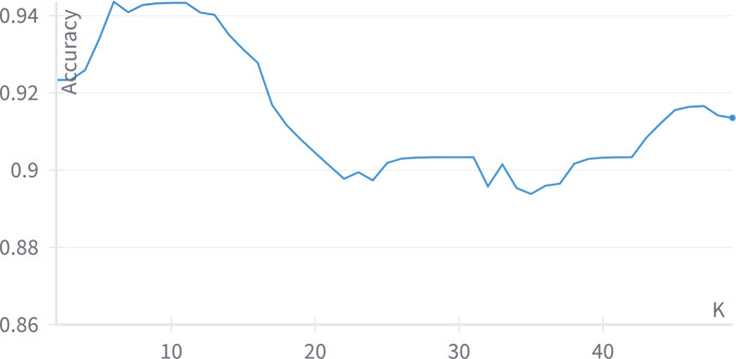 Figure 10
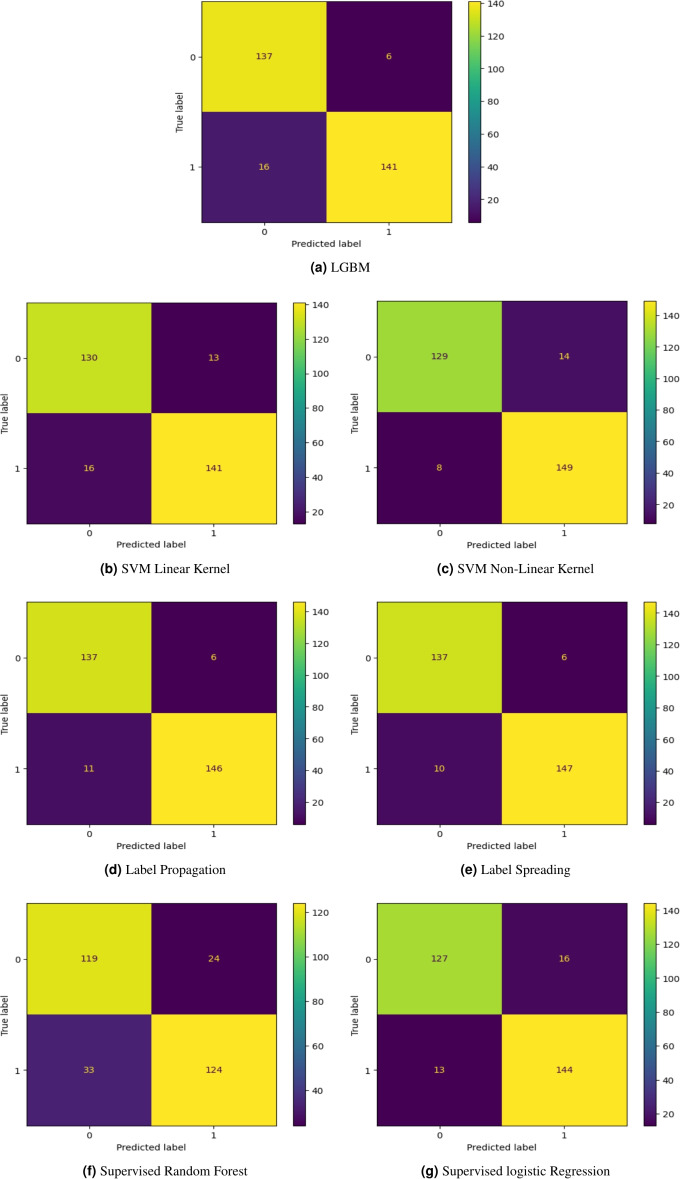 Figure 11
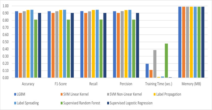 Figure 12
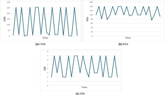 Figure 1
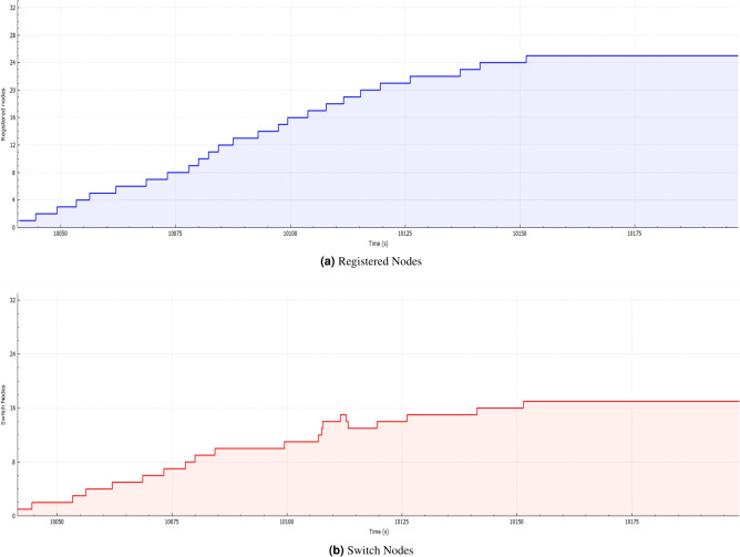 Figure 2
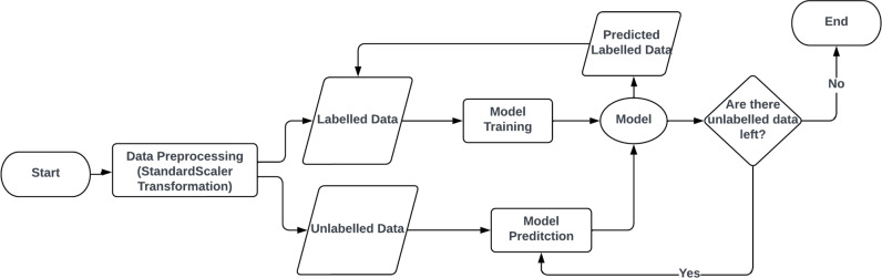 Figure 3
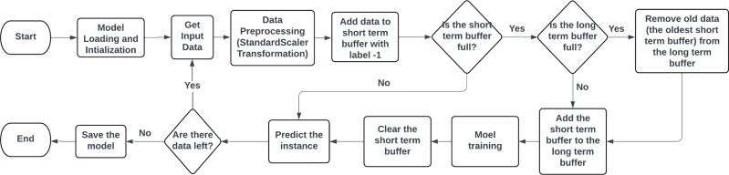 Figure 4
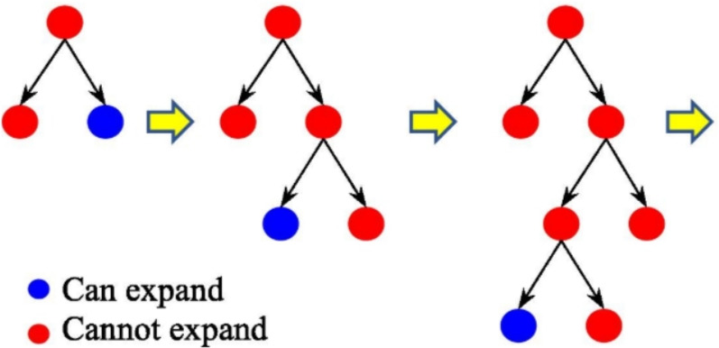 Figure 5
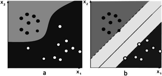 Figure 6
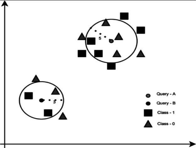 Figure 7
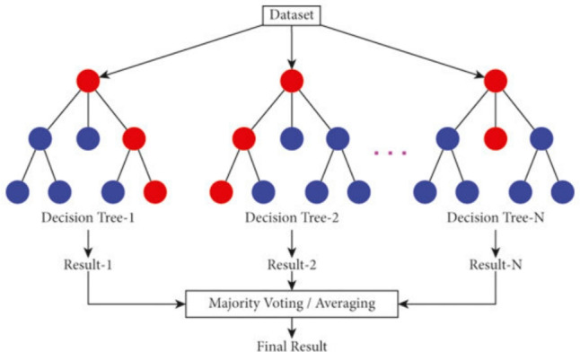 Figure 8
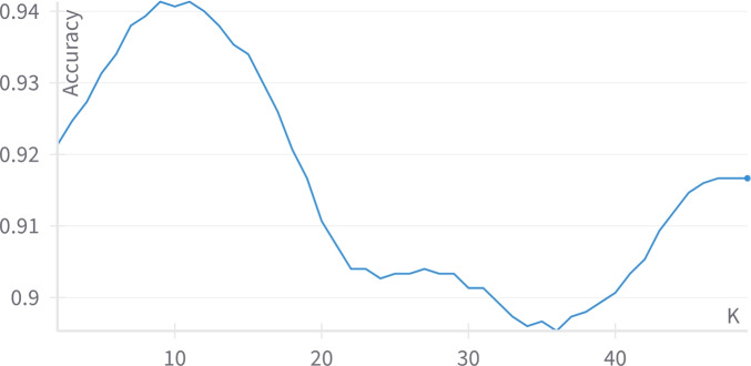 Figure 9
- —Zewail City of Science & Technology
Peer Reviews
No public reviews on file for this paper yet. If you reviewed it on a platform where reviews are public (OpenReview, ICLR, NeurIPS, ICML), you can paste yours below so the community can read it here.
Videos
No videos yet. Explain this paper in a talk, walkthrough, or lecture? Add one.
Taxonomy
TopicsBlind Source Separation Techniques · Power Line Communications and Noise · Vehicle License Plate Recognition
Introduction
In Power Line Communication, data is transferred using the power grid^1^. It is applied in several applications, including smart grids, industrial automation, appliance control, and home lighting^2,3^. The data is transmitted in several stages. The sender has the data modulated to a high-frequency signal. Then, a coupling capacitor and combined filters load the signal to the transmission line. The receiver demodulates the signal^4^. PLC is categorized into two categories, which are Narrow-band and Broadband^5^. Narrow-band has a frequency range of 3 to 500 kHz^6^. The frequency of the broadband ranges from 1.8 to 250 MHz^7^.
The power line communication transmission faces difficult conditions like high interference and low working conditions. A PLC node becomes unavailable due to several factors, including the noise caused by appliances that reduce the SNR, network collisions, and power outages. The nonuniform distribution of the power lines and different load equipment types at the branch points cause attenuation characteristics^8–12^.
PLC nodes may not be in their ideal condition to be read properly. The cost of sending data to an unavailable node is high. Machine learning can be used in detecting the availability of a node. Machine learning is allowing the computer to learn through a pattern. Supervised learning algorithms and Unsupervised Learning are two types of machine learning. In supervised learning, the computer is given a set of features and a mapped vector of the labels. The machine can learn by adjusting its weight to fit the pattern in the given data^13,14^. In unsupervised learning, the data is given to the computer unlabeled with no classes, and the computer model detects the patterns between the data and groups them into clusters^15,16^.
Applying artificial intelligence in predicting the availability of power line communications nodes. The authors of^17^have conducted a comparative study between several machine learning algorithms representing the statistical, regression, Vector-based, predictive, and decision algorithms. They have trained adaptive boosting, the Support Vector Machine (SVM) linear kernel and the SVM non-linear kernel, the random forest and decision trees, K-Nearest Neighbors on a dataset consisting of 1000 readings based on their SNR, CINR, and RSSI with labels 0 for down and 1 for up. The results reached were the ADA algorithm reaching 0.86613, 87%, 0.8646, and 0.9 for the f1-score, accuracy, recall, and precision respectively. The authors of^18^applied clustering, which naturally groups similar data into clusters depending on metrics for similarity^19^. They applied the clustering algorithms on the MIMO NB noise database to check the usefulness of automatic clustering of the PLCs’ multi-conductor noise. They created a feature library. Box Plots and Principal Component Analysis (PCA) have been used to evaluate the features to determine which features are worth to be considered. Box plot summarizes the data on a graph based on six metrics, which are the minimum, median, 25 th and 75 th percentiles, outlier, and maximum. It showed that the data of the feature 5, which is the Samples Skewness, and the feature 7 which is the Samples Pearson correlation are visibly separated. Hierarchical clustering, CURE clustering, which refers to clustering using representatives, and self-organizing map (SOM) have been used in clustering. Hierarchical clustering groups each data point in a separate cluster. Then the distance between each of the two clusters is calculated, and the closest two clusters are grouped in a cluster, and this process is iterated till all the points are in one cluster, forming a tree of clusters called a dendrogram^20,21^. In CURE clustering, the data are clustered initially, and then representative points for each cluster that are far from each other are shrunk by being moved 20% towards the centroid, and then the nearby clusters are grouped^22,23^. In SOM, a network of nodes is formed whose weights are being updated, allowing the nodes to be more similar to the represented data till they reach a map that shows the data clustered according to the similarity^24,25^. The data has been clustered, and the clusters have been labeled according to the probability density to be 35% normal, 23% Middleton Class A, 13% Generalized Extreme Value, 27% Alpha Stable, and 2% unknown.
The conditions of a PLC node may differ throughout time due to the surrounding conditions, which suggests the continuously of the learning of the model to better predict the node availability which is occur in the semi-supervised learning. It is giving the computer, some labeled data and some unlabeled data such that it learns from the labeled data and according to this training, it labels the unlabeled data, and the newly labeled data with high confidence are considered part of the labeled subset of the data and retrain the model and then label new data and so on^26–28^. A dataset has been collected in this work. It consists of 2000 instances of node readings in a 500-node network, which were implemented by Microchip technology PL360 PLC transceiver using the PRIME standard. Self-training, semi-supervised learning approach is proposed to predict the availability of a power line communication node by training and comparing between Supervised learning algorithms (Random Forest and Logistic Regression) and self-training classifiers which are light gradient boosting machine, support vector machine (linear and non-linear kernels), label propagation, and label spreading on a PLC node availability collected dataset by considering the readings of the Carrier to Interference-plus-Noise (CINR), Signal to Noise Ratio (SNR), and Received Signal Strength Indicator (RSSI). Predicting the availability of a node saves time and power due to the high cost of sending data to an unavailable node.
The model details, the dataset, and the algorithms are explained in section 2. In Section 3, the behavior of the models is shown and discussed. The paper is concluded in section 4.
Methodology
Dataset
The dataset consists of 2000 readings of a node in a network consisting of 500 nodes that was implemented by Microchip technology PL360 PLC transceiver using the PRIME standard. The dataset instances consist of CINR, SNR, and RSSI as the features and labels, which indicate whether the node has optimum reading or not, such that 1 represents ’UP’ and 0 represents ’Down’ as shown in Table 1. 50% of the data are for label 0 and the other 50% for label 1. The data is divided into 85% - 15% for the training and testing data, respectively. 15% of the training data has been passed to the semi-supervised learning models as unlabeled data. A subset of the dataset has been selected to plot the features over time, as shown in Figure 1. The correlation between the features has been analyzed, and as table 2 shows, there is a high correlation between the features. Figure 2 shows the number of registered nodes in a specific time instance such that the registered nodes are shown in Figure a and switch nodes are in Figure b. As Figure 2 shows, the more the number of registered nodes changes, the more the number of switch nodes changes.Table 1. Sample of the Dataset.SNRCINRRSSILabel2075031399120750316100−1312991
Fig. 1. The values of the features of the dataset over time. Table 2. Corelation Matrix between the dataset features.SNRCINRRSSISNR10.9750975720.923504485CINR0.97509757210.941400059RSSI0.9235044850.9414000591
Fig. 2. The activity of registered and switch nodes over Time.
The model
As Figure 3shows, the data are split into labeled data and unlabeled data. Then, the model is trained on the labeled data, then predicts a subset of the unlabeled data to be added to the labeled data to retrain the model, then it checks whether there are unlabeled data left or not, and the process iterates till all the unlabeled data are labeled. Semi-supervised Learning is divided into Transudative graph-based methods and inductive methods which is divided into wrapper methods, unsupervised preprocessing, intrinsically semi-supervised^29^. In this research, transudative graph-based methods and inductive wrapper methods are selected. Label Propagation, and Label Spreading representing the transudative graph-based methods and the wrapper methods are represented by Self-Training Classifier with Support Vector Machine (SVM) with linear and non-linear kernel, Light Gradieint Boosting Machine (LGBM) Label propagation algorithm and Label Spreading used K-Nearest Neighbours (KNN) such that labeled and unlabelled data as points on a graph such that the model labels the unlabeled data according to the nearby labeled points, but Label spreading adds regularization to avoid overfitting. Self-Training Classifier uses SVM and LGBM algorithms to predict the unlabeled data^30,31^. As a future work, the model shall be deployed on Raspberry Pi. The overview of the flow that the model is trained on is that batches of the data are collected in the short-term buffer, and all the batches are collected in the long-term buffer. Figure 4 shows the flow of the model when deployed in real life. The trained model is loaded, and long-term and short-term buffers are initialized. New data are processed and then added to the short-term buffer with −1 as a label. Then, checks if the short-term buffer is full; if true, it checks whether the long-term buffer is full or not. If it is full, it removes the oldest data, which is the oldest short buffer, and then the short buffer is added, and the model is trained. The short-term buffer is cleared, and then the instance is predicted. The model is saved if there is no data left and reloaded again after a constant period of time.Fig. 3. Model Flowchart.Fig. 4. Flowchart of training of the model in real-life.
Algorithms
Light Gradient-Boosting Machine (LGBM)
LGBM is a gradient boosting algorithm that depends on decision trees. The model is lightweight as it depends on Exclusive Feature Bundling (EFB) and Gradient-based One-Side Sampling (GOSS). EFB merges the mutually exclusive sparse features, so the number of features is reduced. GOSS selects the data instances that has large gradient to have high gain instead of scanning all data which lead to decreasing the data size, so the algorithm expands the decision tree leaf-wise as shown in Figure 5which leads to a faster training time up to twenty times compared to the conventional gradient boosting decision trees^32,33^.Fig. 5. Leaf-wise Tree Growth^34^.
Support Vector Machine (SVM)
Support Vector Machine separates the data when they are not separable in their dimension into a high dimension. This separation divides them into classes, which is done using a kernel. The kernels can be a non-linear kernel, as shown in Figure 6 - a, and can be a linear kernel, as shown in Figure 6- b^35,36^.Fig. 6. Non-linear and linear kernels of support vector machine^37^.
K-Nearest Neighbors (KNN)
The KNN algorithm predicts the class of the input based on the most similar K points’ features. Figure 7shows the effect of choosing the value of k on the predicted class. When K=3, the input point is predicted as class 1 because between the nearest 3 points, the majority class is class 1. When K=5, the predicted class is class 0, as it is the majority class of the nearest 5 points. To have the best results, the model has to be tested for several values of Ks^38,39^.Fig. 7K-Nearest Neighbors^39^.
Random forest
Random Forest is an ensemble learning algorithm. As shown in Figure 8, it consists of decision trees such that each tree has a random subset of the data instances and features. Each tree gives a classification as a voting, and then the majority voting is the predicted class^40,41^.Fig. 8. Random Forest Algorithm^42^.
Logistic regression
It is a method for binary classification. It predicts the probability of the occurrence of a class. It is the sigmoid function of the linear combination of features with weights as shown in equation (1)^43–45^.
\documentclass[12pt]{minimal} \usepackage{amsmath} \usepackage{wasysym} \usepackage{amsfonts} \usepackage{amssymb} \usepackage{amsbsy} \usepackage{mathrsfs} \usepackage{upgreek} \setlength{\oddsidemargin}{-69pt} \begin{document}$$\begin{aligned} \sigma \left( \sum _{i=1}^{n} w_i x_i + b \right) = \frac{1}{1 + e^{-\left( \sum _{i=1}^{n} w_i x_i + b \right) }} \end{aligned}$$\end{document}Results
As table 3 shows, the best predictions are predicted by Label Spreading. Label Spreading has an average class accuracy equals 94.67%, F1-score equals 0.947, precision equals 0.946, the recall is 0.947, training time=0.018 sec. and the memory consumption is 0.99 MB. The least results resulted by a semi-supervised model were predicted by SVM with a linear kernel. It has an accuracy equals 90.33%, F1-score equals 0.903, precision equals 0.903, recall equals 0.904, training time=0.110 sec., and the memory consumption is 0.99 MB. The number of threads used for training the model has been limited to 4 as in the future, the model shall be deployed on a Raspberry Pi. The self-training classifier has 90% confidence, as the maximum iterations are adjusted to None such that it continues running till no unlabeled data are left. The label propagation and label spreading had the KNN kernel with K equals 9 and 6 respectively as shown in Figures 9 and 10 as a comparison between the different Ks has been conducted ranging between 2 and 49 to determine the best value of K resulting into the best accuracy.Fig. 9. The effect of changing the value of K on the label propagation accuracy.Fig. 10. The effect of changing the value of K on the label spreading accuracy.
Light gradient-boosting machine
Light Gradient-Boosting Machine predicted 137 instances out of 143 correctly for label 0 and 141 for label 157 for label 1 as Figure 11 - a shows.
SVM
Support vector machine has been trained with linear kernel and non-linear kernel. Support vector machine using linear kernel predicted 130 instances out of 143 correctly for label 0 and 141 for label 157 for label 1 as Figure 11 - b shows. Figure 11 - c shows that the model predicted 129 out of 143 for label 0 correctly and 149 out of 157 correctly for label 1.
Label propagation
The model predicted 137 instances for label 0 out of 143 correctly and 146 instances out of 157 for label 1, as Figure 11 - d shows.
Label spreading
As Figure 11 - e shows, the model predicted 137 out of 143 instances correctly to predict label 0 and 147 out of 157 for label 1.
Supervised random forest
It predicted 119 instances out of 143 correctly for label 0 and 124 for label 157 for label 1 as Figure 11 - f shows.
Supervised logistic regression
It predicted 127 instances out of 143 correctly for label 0 and 144 for label 157 for label 1 as Figure 11 - g shows.Fig. 11. Confusion Matrices for the Trained Models.
Discussion
As shown in Table 3 and Figure 12, the best accurate model, Label Spreading, is the most accurate model. It has a regularization phase, which deals with noise. It has an accuracy of 94.67%, an f1-score equals 0.947, a precision is 0.946, and recall equals 0.947 with training time equals 0.018 sec. and memory consumption equals 0.99 MB. A couple of Supervised Learning models have been trained on the same dataset (excluding the unlabeled data) to be compared with the semi-supervised learning models. The supervised learning models are Random Forest and Logistic Regression. Random Forest has an accuracy of 81%, an f1-score equals 0.81, a precision equals 0.81, a recall equals 0.811, a training time is 0.477 seconds, and memory consumption equals 0.99 MB. Logistic Regression’s accuracy is 90.33%, the f1-score is 0.903, precision is 0.904, recall is 0.903, training time equals 0.007 sec, and the memory consumption is 0.99 MB. Both models have yielded lower results than the trained semi-supervised learning models. Although the logistic regression has the least training time, it yielded 90.33% accuracy, while the best semi-supervised learning trained model, which is the label spreading, resulted in 94.67%.Table 3. Numeric results of the trained models.AlgorithmAccuracyF1-ScoreRecallPercisionTraining Time (sec.)Memory (MB)LGBM92.67%0.9270.9280.9270.1950.99SVM Linear Kernel90.33%0.9030.9040.9030.1100.99SVM Non-Linear Kernel92.67%0.9260.9260.9280.3860.99Label Propagation94.33%0.9430.9440.9430.0120.99Label Spreading94.67%0.9470.9470.9460.0180.99Supervised Random Forest81.00%0.8100.8110.8100.4770.99Supervised Logestic Regression90.33%0.9030.9030.9040.0070.99
Fig. 12. Comparison of the performance of the trained models.
Conclusion
PLC communication is the transfer of data using power lines. PLC nodes face conditions that make it unavailable in some time slots. Detecting these time slots earlier saves time. Machine learning can do this detection, but the problem is that the availability of PLC nodes changes due to the surrounding environment, including noise, collisions, or power outages. False predictions in real life, when data is sent to an unavailable node, time and power are consumed as the data are retransmitted to another node. An AI model needs to be trained continuously to better predict the availability of a node. In this paper, a semi-supervised machine learning approach has been introduced. Label propagation, label spreading, and self-training classifier have been used with Light Gradient Boosting Machine and Support Vector Machine (linear and non-linear kernel) algorithms. The algorithms were trained on a dataset consisting of 2000 instances of CINR, SNR, and RSSI as features and node up/down as a label such that 85% of the data are training set and the rest are testing set. 15 % of the training set were unlabeled. Label Spreading had the best results with an accuracy of 94.67%, f1-score equals 0.947, precision is 0.946, and recall equals 0.947 with training time equals 0.018 sec. and memory consumption equals 0.99 MB. The models have been compared to the supervised learning Random Forest and Logistic regression. Logistic Regression performed better than the Random Forest but had less accurate results than the label spreading, achieving an accuracy of 90.33%, an f1-score equals 0.903, precision is 0.904, recall is 0.903 with training time equals 0.007 sec. and memory consumption equals 0.99 MB. As a future work, the model shall be deployed on a Raspberry Pi.
The reference list from the paper itself. Each links out to its DOI / PubMed record.
- 1Chehri, A. spsampsps Zimmermann, A. Spectrum management of power line communications networks for industrial applications. In Zimmermann, A., Howlett, R. J. spsampsps Jain, L. C. (eds.) Human Centred Intelligent Systems, 173–182 (Springer Singapore, Singapore, 2021).
- 2Aderibole, A. O., K. Saathoff, E., J. Kircher, K., B. Leeb, S. & K. Norford, L. Power line communication for low-bandwidth control and sensing. IEEE Transactions on Power Delivery 37, 2172-2181, 10.1109/tpwrd.2021.3106585 (2022).
- 3Aderibole, A. O., K. Saathoff, E., J. Kircher, K., B. Leeb, S. & K. Norford, L. Power line communication for low-bandwidth control and sensing. IEEE Transactions on Power Delivery 37, 2172-2181, 10.1109/tpwrd.2021.3106585 (2022).
- 4ABDALLA, A., Ibwe, K., Gadiel, G. M. & Ally, A. Data communication over power-lines: A review on technical, and applications challenges. Tanzania Journal of Engineering and Technology 43, 46-57, 10.52339/tjet.v 43i 2.971 (2024).
- 5Sharipov, R. R. & Panchenko, O. V. Problems of using plc technology in industrial systems in the context of digitalization. 2024 International Russian Smart Industry Conference (Smart Industry Con) 506-510, 10.1109/smartindustrycon 61328.2024.10515456 (2024).
- 6Elmogy, A. M., Tariq, U., Mohammed, A. & Ibrahim, A. Fake reviews detection using supervised machine learning. International Journal of Advanced Computer Science and Applications 12, 10.14569/ijacsa.2021.0120169 (2021).
- 7Moussa, K. et al. A comparative study of predicting the availability of power line communication nodes using machine learning. Scientific Reports 13, 10.1038/s 41598-023-39120-7 (2023).10.1038/s 41598-023-39120-7PMC 1040351037542096 · doi ↗ · pubmed ↗
- 8Righini, D. & Tonello, A. M. Automatic clustering of noise in multi-conductor narrow band plc channels. 2019 IEEE International Symposium on Power Line Communications and its Applications (ISPLC)10.1109/isplc.2019.8693272 (2019).