Generating diversity and securing completeness in algorithmic retrosynthesis
Florian Mrugalla, Christopher Franz, Yannic Alber, Georg Mogk, Martín Villalba, Thomas Mrziglod, Kevin Schewior

TL;DR
This paper introduces a new algorithm for chemical synthesis planning that improves diversity and efficiency compared to existing methods.
Contribution
The paper introduces a novel chemical diversity score and adapts DFPN to improve diversity and completeness in retrosynthesis planning.
Findings
The proposed algorithm outperforms Monte-Carlo Tree Search in diversity and time efficiency.
DFPN is shown to be complete when reinforced with a threshold-controlling routine.
A cleaner example of DFPN's incompleteness is provided.
Abstract
Chemical synthesis planning has considerably benefited from advances in the field of machine learning. Neural networks can reliably and accurately predict reactions leading to a given, possibly complex, molecule. In this work we focus on algorithms for assembling such predictions to a full synthesis plan that, starting from simple building blocks, produces a given target molecule, a procedure known as retrosynthesis. Objective functions for this task are hard to define and context-specific. In order to generate a diverse set of synthesis plans for chemists to select from, we capture the concept of diversity in a novel chemical diversity score (CDS). Our experiments show that our algorithm outperforms the algorithm predominantly employed in this domain, Monte-Carlo Tree Search, with respect to diversity in terms of our score as well as time efficiency. We adapt Depth-First Proof-Number…
Genes, proteins, chemicals, diseases, species, mutations and cell lines named across the full text — each resolved to its canonical identifier and authoritative record.
Click any figure to enlarge with its caption.
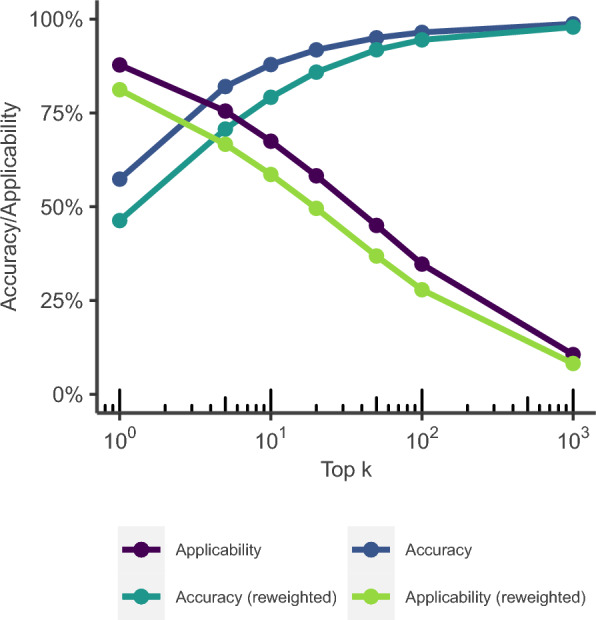 Figure 10
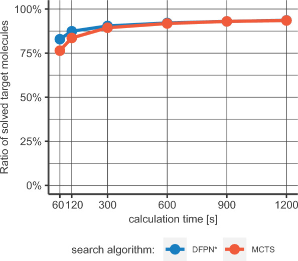 Figure 11
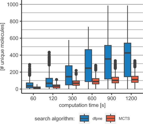 Figure 12
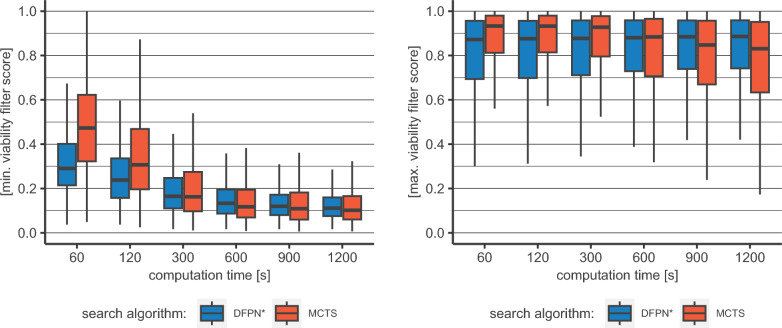 Figure 13
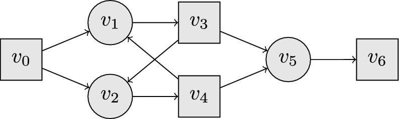 Figure 1
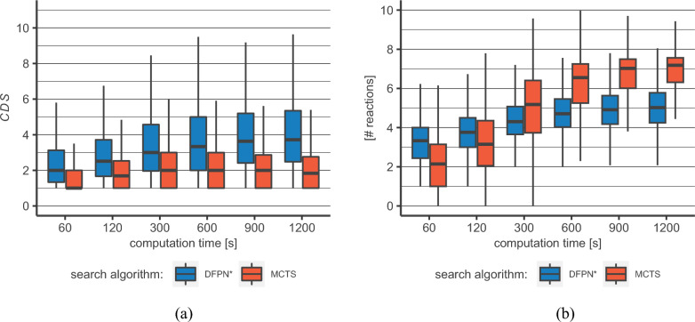 Figure 2
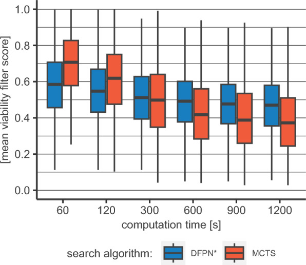 Figure 3
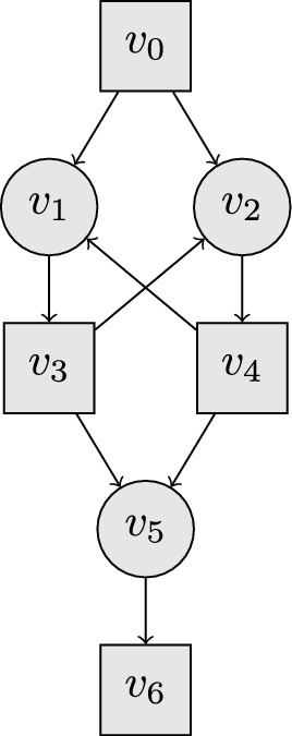 Figure 4
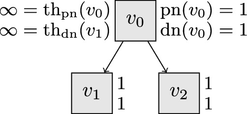 Figure 5
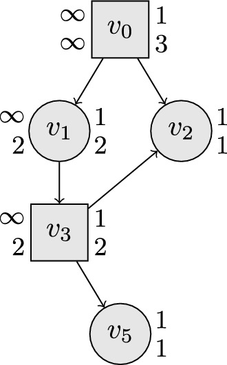 Figure 6
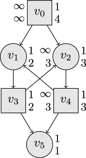 Figure 7
 Figure 8
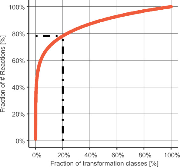 Figure 9
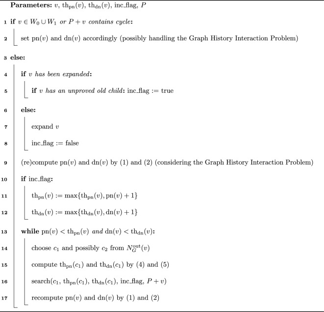 Figure 14
- —http://dx.doi.org/10.13039/501100011958Danmarks Frie Forskningsfond
Peer Reviews
No public reviews on file for this paper yet. If you reviewed it on a platform where reviews are public (OpenReview, ICLR, NeurIPS, ICML), you can paste yours below so the community can read it here.
Videos
No videos yet. Explain this paper in a talk, walkthrough, or lecture? Add one.
Taxonomy
TopicsComputational Drug Discovery Methods · Machine Learning in Materials Science · Chemical Synthesis and Analysis
Introduction
In organic chemistry, one of the most important problems consists in constructing a synthesis plan for a given molecule. Retrosynthesis constitutes a formal approach to this problem: One recursively deconstructs the molecule into building blocks that are readily available for purchase or easy to make. This reverse approach was originally introduced by Corey et al. in the late 1960 s, and it is by now a cornerstone technique in organic chemistry [1–3]. Yet, applying this technique in practice is a highly complicated task due to a large number of potentially relevant reactions as well as multiple constraints (building-block availability, functional-group protection, safety regulations, green-chemistry considerations), and it has traditionally required solid human expertise. In the last decade, however, the field of Computer-Assisted Synthesis Planning (CASP) underwent significant improvements driven by the successful combination of advances in machine learning and the availability of sufficient amounts of reaction data [4–11].
There are two predominant approaches for building a CASP tool, template-based and template-free. Template-based approaches encode reactions as the chemical landscape around a reaction center, which can be extracted either manually by experts or with a data-driven approach [5, 9]. These templates can be used during a retrosynthetic search in a recursive fashion to derive new intermediates and starting molecules of suitable complexity and availability. Template-free approaches, in contrast, do not rely on handcrafted or automatically extracted transformation rules. Following tools and approaches developed by the Natural Language Processing (NLP) community, a set of SMILES (words, reactants) is transformed into another set of SMILES (words, products) [12]. Coupling this one-step synthesis model with a powerful search algorithm has been shown to yield similar performance as the aforementioned methods [10].
In 2018, Segler et al. [9] showed the viability of a data-driven approach, using two neural networks: the first one to predict which transformation templates should be prioritized during the route search and the second one to grade them according to their plausibility. These advances were followed by copious research mostly concerned with the quality of these neural networks and how they ingest their input data, e.g., regarding the usage of transformation templates [5, 6, 10, 12–14].
This work considers the overall quality of the found synthesis plans more directly. The quality of a synthesis plan depends on a large number of aspects such as safety, yield, required level of expertise, and available laboratory equipment, whose levels of relevance may vastly differ depending on context. It is therefore extremely difficult to capture this concept in a formal definition. Our approach circumvents this issue and can be summarized as quality through diversity. That is, we aim to find not just a single synthesis plan but several of them, maximizing the diversity—a concept we formally define—in the set of plans that we generate. Chemists can then pick a synthesis plan or recombine chemical ideas present in the set of plans, to meet the criteria relevant in the context at hand.
This diversity is possible thanks to more than 250 years of chemical research leading to multiple known ways to synthesize a molecule, target compound, or intermediate from commercially available building blocks. Unfortunately, this also poses a selection problem in each retrosynthesis step due to the overwhelmingly large host of choices that has to be explored to find a single solution, let alone a diverse set of them. Multiple algorithms, many of them viewing retrosynthesis as a two-player game, were proposed to solve this problem [9, 15, 16]. The most commonly used one is Monte-Carlo Tree Search [6, 9, 17]. While this algorithm can reliably find multiple solutions, it is not clear whether this set of solutions turns out diverse.
Instead of MCTS, we consider Depth-First Proof-Number Search (DFPN) [18], a popular [19, 20] and more efficient variant of Proof-Number Search (PNS) [21]. A version of DFPN has also been successfully applied to retrosynthesis [16], but PNS and its variants just stop after finding the first solution. We introduce an adaptation to this algorithm which can be applied essentially to any version of PNS, whose output will be a set of solutions, with explicit focus on diversity. In the experimental part of our paper, we indeed find that our version, called DFPN*, generally outperforms MCTS with respect to our diversity score, but in fact also with respect to efficiently finding the first synthesis plan.
To make a case for DFPN and its variants, we also solve an open problem regarding it as a side result: It can be shown that (plain) DFPN is not complete [22], i.e., it is possible that there exists a solution, but DFPN runs into an infinite loop rather than outputting the solution. (We give a much smaller example showing that.) Refinements of DFPN that have seemed to be complete in experiments are df-pn(r) [23] and DFPN with the Threshold Controlling Algorithm (TCA) [24], but no proofs of completeness for such variants are known. We provide a proof of completeness for DFPN with TCA.
Methods
In this section, we first discuss how to measure diversity, then how to reduce retrosynthesis to solving two-player games, then how to solve such games (especially through DFPN), and finally how to adapt DFPN to find sets of (diverse) solutions.
Measuring diversity in pathways
Practicing chemists have a good intuitive notion of chemical diversity. However, it is challenging to formally define the diversity of a set of synthesis pathways fitting this intuition. Nonetheless, diversity is a key objective for current, actively used CASP tools. A broadly applicable metric is necessary to not rely on anecdotal observations [25] alone to track algorithmic changes towards higher diversity in said sets of synthesis pathways. Some efforts towards this where made before. A natural approach to the problem is to measure the diversity among the molecules [26, 27] appearing in the routes or simply count unique intermediates and building blocks. In Table 4 and Fig. 12 in the appendix, we provide the respective numbers for both algorithms studied here with respect to the search times. Such metrics are, however, not practical. Structural variations in reactants tend to be overemphasized as they may not alter the chemical nature of the reactions (e.g., different protection or leaving groups fulfilling the same purpose). Another approach to compare routes with each other is to calculate their graph edit distance or tree edit distance [28, 29]. A subsequent clustering on the corresponding distance matrix can be used to asses the diversity within a set of routes [30]. While the higher abstraction level allows for an increased focus on relevant difference between routes and therefore also improves the associated diversity metric, it also comes with its own drawbacks. First, the metric can go down by adding further routes to the set [31] which is, from a theoretical point of view, plausible but goes beside the point of gauging which set is more useful for lab practitioners. Second, while being a very elegant way of measuring distances between routes from a mathematical point of view, the graph edit distance is indiscriminate towards the importance of differences between routes from a chemical perspective. A very strict way to tackle the problem is to count only the number of routes with no overlap, as proposed by Maziarz et al. [31]. In our context, this is however too restrictive since potentially important chemical solutions can go unrecognized by the metric when paired with an already used reaction.
We have worked in close collaboration with several lab chemists from multiple different fields such as medicinal, agricultural, and process chemistry to formalize our approach to measure route diversity. The general understanding among lab chemists can be summarized as the number of different chemical ideas observed between the individual synthesis pathways. Unfortunately, chemical ideas are a similarly vague concept as diversity and therefore difficult to distinguish and count objectively.
For this reason we propose a new metric, dubbed Chemical Diversity Score CDS, based on the intuitive idea of disconnections (bond breakages) which was used in similar contexts before [10, 32]. The core idea is to mimic the thought process involved in a manual retrosynthesis analysis, making it quantifiable.
By identifying which bonds of a molecule get broken from the retrosynthesis point of view (i.e. formed in forward direction) in any given pathway, we keep track of the synthesis approaches present in a set of routes. We choose to focus on the final result of the route search (sets of full routes) over focusing on the diversity coming from the individual parts (like the reaction prediction model) of a given CASP tool. Model metrics do not necessarily have much bearing on the route search results (as demonstrated in Fig. 10 and Table 3) and gains achieved here might easily be overwritten by other parts of the pipeline like filtering mechanisms or the search algorithm itself. Figure 10 and Table 3 of Appendix D.5 lend support to our choice. Similar observations were made by Genheden and Bjerrum [29] and Maziarz et al. [31].
As a result, the higher chemical concept is still recognized while avoiding an artificially high diversity. For example, a famous and often used reaction type is the Suzuki-coupling [33]. There are about 20 variants of this technique to create the same carbon-carbon bond, which can lead to different synthesis routes, but which are all based on the same chemical idea. Based on our discussions with lab chemists, we consider the level of abstraction provided by the disconnections ideal, as they do not discriminate between different named reactions forming the same bond, but are still capturing different synthesis strategies.
To compute the \documentclass[12pt]{minimal} \usepackage{amsmath} \usepackage{wasysym} \usepackage{amsfonts} \usepackage{amssymb} \usepackage{amsbsy} \usepackage{mathrsfs} \usepackage{upgreek} \setlength{\oddsidemargin}{-69pt} \begin{document}$$\text{CDS}$$\end{document} , all bonds formed in the proposed synthesis pathway get identified and labeled. From the resulting sets we select those which cannot be represented by another, smaller set of bonds found in all the pathways for the target molecule. This way, we eliminate miscellaneous reactions that do not contribute to the chemical diversity in a meaningful way, forming the set \documentclass[12pt]{minimal} \usepackage{amsmath} \usepackage{wasysym} \usepackage{amsfonts} \usepackage{amssymb} \usepackage{amsbsy} \usepackage{mathrsfs} \usepackage{upgreek} \setlength{\oddsidemargin}{-69pt} \begin{document}$$C_M$$\end{document} . The final score is then obtained by calculating the mean over the all-to-all Jaccard distance matrix expressed by
\documentclass[12pt]{minimal} \usepackage{amsmath} \usepackage{wasysym} \usepackage{amsfonts} \usepackage{amssymb} \usepackage{amsbsy} \usepackage{mathrsfs} \usepackage{upgreek} \setlength{\oddsidemargin}{-69pt} \begin{document}$$\begin{aligned} \text {CDS}:= 1 + \frac{1}{|C_M|} \sum _{T \in C_M}\sum _{T' \in C_M} d_J(\hat{T},\hat{T}'). \end{aligned}$$\end{document}The \documentclass[12pt]{minimal} \usepackage{amsmath} \usepackage{wasysym} \usepackage{amsfonts} \usepackage{amssymb} \usepackage{amsbsy} \usepackage{mathrsfs} \usepackage{upgreek} \setlength{\oddsidemargin}{-69pt} \begin{document}$$\text {CDS}$$\end{document} can be interpreted as the number of different chemical ideas present in a given set of synthesis pathways. Higher \documentclass[12pt]{minimal} \usepackage{amsmath} \usepackage{wasysym} \usepackage{amsfonts} \usepackage{amssymb} \usepackage{amsbsy} \usepackage{mathrsfs} \usepackage{upgreek} \setlength{\oddsidemargin}{-69pt} \begin{document}$$\text {CDS}$$\end{document} values are considered better, as they indicate a higher diversity between them. A more detailed mathematical formulation and further explanations can be found in Appendix 4.1.
Game-theoretical approaches to the retrosynthesis problem
Viewing retrosynthetic planning as games on a simple directed graph is a standard approach (e.g., [9, 16]). In the two-player game which we focus on in this paper, there is a node for every molecule and a node for every reaction. We will call one player molecule player and the other reaction player. The game starts at the node corresponding to the target molecule. It is the molecule (reaction) player’s turn whenever the game is at a molecule (reaction) node. The next node can be chosen according to the following directed edges: From a molecule node, the edges lead to all nodes corresponding to reactions having the molecule corresponding to the current node as product. From a reaction node, the edges lead to all nodes corresponding to reactants required for the reaction corresponding to the current node. The molecule player wins if a node corresponding to a building block is reached, and the reaction player wins if a dead end (i.e., a molecule that can neither be synthesized nor bought) is reached or a node is visited for the second time. This way, a winning strategy for the molecule player represents a synthesis plan for the target molecule. Conversely, if there exists a winning strategy for the reaction player, the target molecule cannot be synthesized with the reactions represented in the graph. For this emerging two-player game, PNS was first used in its regular form [15], whereas DFPN was first applied as part of the DFPN-E algorithm [16] and later within the CompRet tool [8]. In the next chapter, we will explain the (DF)PNS in more detail.
In what can be interpreted as a one-player game, a node usually corresponds to a set of molecules and each edge to a reaction. Monte-Carlo Tree-Search [9, 34] operates iteratively on such games, where each iteration consists of four steps: The first one is selection, where the most promising node gets selected. The second one is expansion, where the previously selected node gets expanded by creating one or more nodes. After that the simulation happens, where starting with these nodes a game to end nodes gets simulated, and lastly the backpropagation, where the result of these games is propagated back in the tree. Already visited nodes get penalized such that, when running for a long period of time, it can also find a set of different synthesis plans.
Very recently, Tripp et al. [35] use a type of greedy algorithm specifically designed for the task of creating multiple synthesis plans with a high probability that at least one of them is feasible, and called it Retro-fallback. Their heuristic can be summarized as simply expanding the molecule that is expected to have the highest increase of their so-called successful synthesis probability (SSP). For a given synthesis plan T, the SSP depends not only on the probability that T is successful, but also incorporates the probability of any of the previously found synthesis plans and whether T can significantly increase it. Other promising results were obtained using variations of A* search [4, 25].
Depth-first proof number search and variants
To find winning strategies, Proof-Number Search (PNS) [21] explores the graph from the start node by iteratively expanding nodes that were previously not expanded. By doing so, PNS learns if the node is winning for one of the players (and if so, which) and explores its out-neighbors. A node is called proved if a winning strategy for the molecule player can be inferred from the explored part of G; if a winning strategy for the reaction player can be inferred, the node is called disproved. A node that is neither proved nor disproved is said to be unproved.
The (dis)proof number of an explored node v is defined to be the minimum number of explored unproved nodes that have to be (dis)proved for v to be (dis)proved. The precise numbers are NP-hard to compute [36]. PNS instead efficiently maintains estimates of these numbers, \documentclass[12pt]{minimal} \usepackage{amsmath} \usepackage{wasysym} \usepackage{amsfonts} \usepackage{amssymb} \usepackage{amsbsy} \usepackage{mathrsfs} \usepackage{upgreek} \setlength{\oddsidemargin}{-69pt} \begin{document}$$\text{pn} (v)$$\end{document} and \documentclass[12pt]{minimal} \usepackage{amsmath} \usepackage{wasysym} \usepackage{amsfonts} \usepackage{amssymb} \usepackage{amsbsy} \usepackage{mathrsfs} \usepackage{upgreek} \setlength{\oddsidemargin}{-69pt} \begin{document}$$\text{dn} (v)$$\end{document} for each node v; \documentclass[12pt]{minimal} \usepackage{amsmath} \usepackage{wasysym} \usepackage{amsfonts} \usepackage{amssymb} \usepackage{amsbsy} \usepackage{mathrsfs} \usepackage{upgreek} \setlength{\oddsidemargin}{-69pt} \begin{document}$$\text{pn} (v)=\text{dn} (v)=1$$\end{document} for unexpanded nodes v such as \documentclass[12pt]{minimal} \usepackage{amsmath} \usepackage{wasysym} \usepackage{amsfonts} \usepackage{amssymb} \usepackage{amsbsy} \usepackage{mathrsfs} \usepackage{upgreek} \setlength{\oddsidemargin}{-69pt} \begin{document}$$v_0$$\end{document} in the beginning. PNS uses \documentclass[12pt]{minimal} \usepackage{amsmath} \usepackage{wasysym} \usepackage{amsfonts} \usepackage{amssymb} \usepackage{amsbsy} \usepackage{mathrsfs} \usepackage{upgreek} \setlength{\oddsidemargin}{-69pt} \begin{document}$$\text{pn} (\cdot )$$\end{document} and \documentclass[12pt]{minimal} \usepackage{amsmath} \usepackage{wasysym} \usepackage{amsfonts} \usepackage{amssymb} \usepackage{amsbsy} \usepackage{mathrsfs} \usepackage{upgreek} \setlength{\oddsidemargin}{-69pt} \begin{document}$$\text{dn} (\cdot )$$\end{document} to determine the most promising node, the next node to expand: Starting from \documentclass[12pt]{minimal} \usepackage{amsmath} \usepackage{wasysym} \usepackage{amsfonts} \usepackage{amssymb} \usepackage{amsbsy} \usepackage{mathrsfs} \usepackage{upgreek} \setlength{\oddsidemargin}{-69pt} \begin{document}$$v_0$$\end{document} , it iteratively selects the out-neighbor with the minimum proof number from a molecule-player node and with a minimum disproof number from a reaction-player node, until reaching a non-expanded node, which then is expanded. PNS then backtracks to \documentclass[12pt]{minimal} \usepackage{amsmath} \usepackage{wasysym} \usepackage{amsfonts} \usepackage{amssymb} \usepackage{amsbsy} \usepackage{mathrsfs} \usepackage{upgreek} \setlength{\oddsidemargin}{-69pt} \begin{document}$$v_0$$\end{document} , updating \documentclass[12pt]{minimal} \usepackage{amsmath} \usepackage{wasysym} \usepackage{amsfonts} \usepackage{amssymb} \usepackage{amsbsy} \usepackage{mathrsfs} \usepackage{upgreek} \setlength{\oddsidemargin}{-69pt} \begin{document}$$\text{pn} (\cdot )$$\end{document} for a molecule-player node to be the minimum \documentclass[12pt]{minimal} \usepackage{amsmath} \usepackage{wasysym} \usepackage{amsfonts} \usepackage{amssymb} \usepackage{amsbsy} \usepackage{mathrsfs} \usepackage{upgreek} \setlength{\oddsidemargin}{-69pt} \begin{document}$$\text{pn}$$\end{document} value of an out-neighbor and for a reaction-player node to be the sum of these \documentclass[12pt]{minimal} \usepackage{amsmath} \usepackage{wasysym} \usepackage{amsfonts} \usepackage{amssymb} \usepackage{amsbsy} \usepackage{mathrsfs} \usepackage{upgreek} \setlength{\oddsidemargin}{-69pt} \begin{document}$$\text{pn}$$\end{document} values (vice versa for \documentclass[12pt]{minimal} \usepackage{amsmath} \usepackage{wasysym} \usepackage{amsfonts} \usepackage{amssymb} \usepackage{amsbsy} \usepackage{mathrsfs} \usepackage{upgreek} \setlength{\oddsidemargin}{-69pt} \begin{document}$$\text{dn}$$\end{document} ). If the graph is an out-tree, PNS exactly determines the proof and disproof numbers in this way.
Depth-First Proof-Number Search (DFPN) [18] does not start the search for the most promising node from \documentclass[12pt]{minimal} \usepackage{amsmath} \usepackage{wasysym} \usepackage{amsfonts} \usepackage{amssymb} \usepackage{amsbsy} \usepackage{mathrsfs} \usepackage{upgreek} \setlength{\oddsidemargin}{-69pt} \begin{document}$$v_0$$\end{document} in each iteration, making it more efficient. Instead, when node v is currently selected, it tries to use thresholds \documentclass[12pt]{minimal} \usepackage{amsmath} \usepackage{wasysym} \usepackage{amsfonts} \usepackage{amssymb} \usepackage{amsbsy} \usepackage{mathrsfs} \usepackage{upgreek} \setlength{\oddsidemargin}{-69pt} \begin{document}$$\text{th}_{\text{pn}} (\cdot )$$\end{document} and \documentclass[12pt]{minimal} \usepackage{amsmath} \usepackage{wasysym} \usepackage{amsfonts} \usepackage{amssymb} \usepackage{amsbsy} \usepackage{mathrsfs} \usepackage{upgreek} \setlength{\oddsidemargin}{-69pt} \begin{document}$$\text{th}_{\text{dn}} (\cdot )$$\end{document} to decide whether the path taken from \documentclass[12pt]{minimal} \usepackage{amsmath} \usepackage{wasysym} \usepackage{amsfonts} \usepackage{amssymb} \usepackage{amsbsy} \usepackage{mathrsfs} \usepackage{upgreek} \setlength{\oddsidemargin}{-69pt} \begin{document}$$v_0$$\end{document} to v is part of a path that PNS would take. In particular, if \documentclass[12pt]{minimal} \usepackage{amsmath} \usepackage{wasysym} \usepackage{amsfonts} \usepackage{amssymb} \usepackage{amsbsy} \usepackage{mathrsfs} \usepackage{upgreek} \setlength{\oddsidemargin}{-69pt} \begin{document}$$\text{pn} (v)<\text{th}_{\text{pn}} (v)$$\end{document} and \documentclass[12pt]{minimal} \usepackage{amsmath} \usepackage{wasysym} \usepackage{amsfonts} \usepackage{amssymb} \usepackage{amsbsy} \usepackage{mathrsfs} \usepackage{upgreek} \setlength{\oddsidemargin}{-69pt} \begin{document}$$\text{dn} (v)<\text{th}_{\text{dn}} (v)$$\end{document} , then it continues the search like PNS would, and otherwise it backtracks one step. The values of \documentclass[12pt]{minimal} \usepackage{amsmath} \usepackage{wasysym} \usepackage{amsfonts} \usepackage{amssymb} \usepackage{amsbsy} \usepackage{mathrsfs} \usepackage{upgreek} \setlength{\oddsidemargin}{-69pt} \begin{document}$$\text{pn}$$\end{document} and \documentclass[12pt]{minimal} \usepackage{amsmath} \usepackage{wasysym} \usepackage{amsfonts} \usepackage{amssymb} \usepackage{amsbsy} \usepackage{mathrsfs} \usepackage{upgreek} \setlength{\oddsidemargin}{-69pt} \begin{document}$$\text{dn}$$\end{document} are only recomputed at the node that DFPN is currently considering. If v only has a single neighbor, the thresholds are simply passed on. Otherwise, if v is a molecule-player node, the \documentclass[12pt]{minimal} \usepackage{amsmath} \usepackage{wasysym} \usepackage{amsfonts} \usepackage{amssymb} \usepackage{amsbsy} \usepackage{mathrsfs} \usepackage{upgreek} \setlength{\oddsidemargin}{-69pt} \begin{document}$$\text{th}_{\text{pn}}$$\end{document} value of the chosen child becomes the minimum of the \documentclass[12pt]{minimal} \usepackage{amsmath} \usepackage{wasysym} \usepackage{amsfonts} \usepackage{amssymb} \usepackage{amsbsy} \usepackage{mathrsfs} \usepackage{upgreek} \setlength{\oddsidemargin}{-69pt} \begin{document}$$\text{th}_{\text{pn}}$$\end{document} value of v and the increment of the proof number of the second-best child. If v is a reaction-player node, the \documentclass[12pt]{minimal} \usepackage{amsmath} \usepackage{wasysym} \usepackage{amsfonts} \usepackage{amssymb} \usepackage{amsbsy} \usepackage{mathrsfs} \usepackage{upgreek} \setlength{\oddsidemargin}{-69pt} \begin{document}$$\text{th}_{\text{pn}}$$\end{document} value of the chosen child becomes the surplus between pn(v) and its threshold plus the \documentclass[12pt]{minimal} \usepackage{amsmath} \usepackage{wasysym} \usepackage{amsfonts} \usepackage{amssymb} \usepackage{amsbsy} \usepackage{mathrsfs} \usepackage{upgreek} \setlength{\oddsidemargin}{-69pt} \begin{document}$$\text{pn}$$\end{document} value of the chosen child. For \documentclass[12pt]{minimal} \usepackage{amsmath} \usepackage{wasysym} \usepackage{amsfonts} \usepackage{amssymb} \usepackage{amsbsy} \usepackage{mathrsfs} \usepackage{upgreek} \setlength{\oddsidemargin}{-69pt} \begin{document}$$\text{dn}$$\end{document} , the operations are again analogous. As before, this is exact for out-trees, but DFPN is incomplete on general graphs [22].
As pointed out in [37], DFPN and PNS as stated above are not necessarily correct on graphs that contain cycles: A proof or a disproof of some node v that is found when v is visited through some path P cannot certainly be reused when v is visited through some path \documentclass[12pt]{minimal} \usepackage{amsmath} \usepackage{wasysym} \usepackage{amsfonts} \usepackage{amssymb} \usepackage{amsbsy} \usepackage{mathrsfs} \usepackage{upgreek} \setlength{\oddsidemargin}{-69pt} \begin{document}$$P'\ne P$$\end{document} . This is called the Graph History Interaction Problem. As a general solution [23, 38], one can, upon (dis)proving a node when visiting it through P, save the (dis)proof only with respect to P. When visiting v again through \documentclass[12pt]{minimal} \usepackage{amsmath} \usepackage{wasysym} \usepackage{amsfonts} \usepackage{amssymb} \usepackage{amsbsy} \usepackage{mathrsfs} \usepackage{upgreek} \setlength{\oddsidemargin}{-69pt} \begin{document}$$P'$$\end{document} , it can be verified if the previously found proof is still valid. For further details, we refer the reader to the aforementioned works.
To break infinite loops, the Threshold Controlling Algorithm (TCA) [24] maintains a value \documentclass[12pt]{minimal} \usepackage{amsmath} \usepackage{wasysym} \usepackage{amsfonts} \usepackage{amssymb} \usepackage{amsbsy} \usepackage{mathrsfs} \usepackage{upgreek} \setlength{\oddsidemargin}{-69pt} \begin{document}$$\text{md} (v)$$\end{document} for every node v. It represents the (minimum) distance between \documentclass[12pt]{minimal} \usepackage{amsmath} \usepackage{wasysym} \usepackage{amsfonts} \usepackage{amssymb} \usepackage{amsbsy} \usepackage{mathrsfs} \usepackage{upgreek} \setlength{\oddsidemargin}{-69pt} \begin{document}$$v_0$$\end{document} and v in the explored part of G. Whenever a node v is visited that has an unproved old child c, i.e., \documentclass[12pt]{minimal} \usepackage{amsmath} \usepackage{wasysym} \usepackage{amsfonts} \usepackage{amssymb} \usepackage{amsbsy} \usepackage{mathrsfs} \usepackage{upgreek} \setlength{\oddsidemargin}{-69pt} \begin{document}$$\text{md} (c)\le \text{md} (v)$$\end{document} , TCA adjusts \documentclass[12pt]{minimal} \usepackage{amsmath} \usepackage{wasysym} \usepackage{amsfonts} \usepackage{amssymb} \usepackage{amsbsy} \usepackage{mathrsfs} \usepackage{upgreek} \setlength{\oddsidemargin}{-69pt} \begin{document}$$\text{th}_{\text{pn}} (v)$$\end{document} and \documentclass[12pt]{minimal} \usepackage{amsmath} \usepackage{wasysym} \usepackage{amsfonts} \usepackage{amssymb} \usepackage{amsbsy} \usepackage{mathrsfs} \usepackage{upgreek} \setlength{\oddsidemargin}{-69pt} \begin{document}$$\text{th}_{\text{dn}} (v)$$\end{document} such that DFPN does not backtrack. In particular, it sets \documentclass[12pt]{minimal} \usepackage{amsmath} \usepackage{wasysym} \usepackage{amsfonts} \usepackage{amssymb} \usepackage{amsbsy} \usepackage{mathrsfs} \usepackage{upgreek} \setlength{\oddsidemargin}{-69pt} \begin{document}$$\text{th}_{\text{pn}} (v)$$\end{document} and \documentclass[12pt]{minimal} \usepackage{amsmath} \usepackage{wasysym} \usepackage{amsfonts} \usepackage{amssymb} \usepackage{amsbsy} \usepackage{mathrsfs} \usepackage{upgreek} \setlength{\oddsidemargin}{-69pt} \begin{document}$$\text{th}_{\text{dn}} (v)$$\end{document} to values so that \documentclass[12pt]{minimal} \usepackage{amsmath} \usepackage{wasysym} \usepackage{amsfonts} \usepackage{amssymb} \usepackage{amsbsy} \usepackage{mathrsfs} \usepackage{upgreek} \setlength{\oddsidemargin}{-69pt} \begin{document}$$\text{pn} (v)<\text{th}_{\text{pn}} (v)$$\end{document} and \documentclass[12pt]{minimal} \usepackage{amsmath} \usepackage{wasysym} \usepackage{amsfonts} \usepackage{amssymb} \usepackage{amsbsy} \usepackage{mathrsfs} \usepackage{upgreek} \setlength{\oddsidemargin}{-69pt} \begin{document}$$\text{dn} (v)<\text{th}_{\text{dn}} (v)$$\end{document} are definitely satisfied. The fact that the thresholds have been increased is passed to subsequent recursive calls of the algorithm, prompting these calls to also increase the corresponding thresholds, until a node is expanded or a cycle is closed (i.e., progress is made).
We give a more formal description of the entire algorithm in a general context in Appendix A.
Completeness of DFPN with TCA
We start this section with (re-)justifying variants of DFPN by giving a counter example to the completeness of DFPN that is significantly simpler than the known counter example [22]. In the second subsection we will then prove completeness of DFPN with TCA.
Simpler counter example without TCA
Fig. 1. The graph G that shows that DFPN is not complete.The molecule nodes and the reaction nodes are depicted as squares and circles, respectively
We consider the graph shown in Fig. 1. In that graph, DFPN visits \documentclass[12pt]{minimal} \usepackage{amsmath} \usepackage{wasysym} \usepackage{amsfonts} \usepackage{amssymb} \usepackage{amsbsy} \usepackage{mathrsfs} \usepackage{upgreek} \setlength{\oddsidemargin}{-69pt} \begin{document}$$v_3$$\end{document} and \documentclass[12pt]{minimal} \usepackage{amsmath} \usepackage{wasysym} \usepackage{amsfonts} \usepackage{amssymb} \usepackage{amsbsy} \usepackage{mathrsfs} \usepackage{upgreek} \setlength{\oddsidemargin}{-69pt} \begin{document}$$v_4$$\end{document} alternating from \documentclass[12pt]{minimal} \usepackage{amsmath} \usepackage{wasysym} \usepackage{amsfonts} \usepackage{amssymb} \usepackage{amsbsy} \usepackage{mathrsfs} \usepackage{upgreek} \setlength{\oddsidemargin}{-69pt} \begin{document}$$v_0$$\end{document} via \documentclass[12pt]{minimal} \usepackage{amsmath} \usepackage{wasysym} \usepackage{amsfonts} \usepackage{amssymb} \usepackage{amsbsy} \usepackage{mathrsfs} \usepackage{upgreek} \setlength{\oddsidemargin}{-69pt} \begin{document}$$v_2$$\end{document} and \documentclass[12pt]{minimal} \usepackage{amsmath} \usepackage{wasysym} \usepackage{amsfonts} \usepackage{amssymb} \usepackage{amsbsy} \usepackage{mathrsfs} \usepackage{upgreek} \setlength{\oddsidemargin}{-69pt} \begin{document}$$v_1$$\end{document} , respectively, in an infinite loop. In particular, it never expands \documentclass[12pt]{minimal} \usepackage{amsmath} \usepackage{wasysym} \usepackage{amsfonts} \usepackage{amssymb} \usepackage{amsbsy} \usepackage{mathrsfs} \usepackage{upgreek} \setlength{\oddsidemargin}{-69pt} \begin{document}$$v_5$$\end{document} . When \documentclass[12pt]{minimal} \usepackage{amsmath} \usepackage{wasysym} \usepackage{amsfonts} \usepackage{amssymb} \usepackage{amsbsy} \usepackage{mathrsfs} \usepackage{upgreek} \setlength{\oddsidemargin}{-69pt} \begin{document}$$W_0=\{v_6\}$$\end{document} and \documentclass[12pt]{minimal} \usepackage{amsmath} \usepackage{wasysym} \usepackage{amsfonts} \usepackage{amssymb} \usepackage{amsbsy} \usepackage{mathrsfs} \usepackage{upgreek} \setlength{\oddsidemargin}{-69pt} \begin{document}$$W_1=\emptyset$$\end{document} , DFPN therefore never discovers the only winning strategy for the molecule player from \documentclass[12pt]{minimal} \usepackage{amsmath} \usepackage{wasysym} \usepackage{amsfonts} \usepackage{amssymb} \usepackage{amsbsy} \usepackage{mathrsfs} \usepackage{upgreek} \setlength{\oddsidemargin}{-69pt} \begin{document}$$v_0$$\end{document} , which includes \documentclass[12pt]{minimal} \usepackage{amsmath} \usepackage{wasysym} \usepackage{amsfonts} \usepackage{amssymb} \usepackage{amsbsy} \usepackage{mathrsfs} \usepackage{upgreek} \setlength{\oddsidemargin}{-69pt} \begin{document}$$v_6$$\end{document} . In this example the TCA would upon visiting \documentclass[12pt]{minimal} \usepackage{amsmath} \usepackage{wasysym} \usepackage{amsfonts} \usepackage{amssymb} \usepackage{amsbsy} \usepackage{mathrsfs} \usepackage{upgreek} \setlength{\oddsidemargin}{-69pt} \begin{document}$$v_3$$\end{document} increase its threshold, since the minimal distance from its child \documentclass[12pt]{minimal} \usepackage{amsmath} \usepackage{wasysym} \usepackage{amsfonts} \usepackage{amssymb} \usepackage{amsbsy} \usepackage{mathrsfs} \usepackage{upgreek} \setlength{\oddsidemargin}{-69pt} \begin{document}$$v_2$$\end{document} to the root \documentclass[12pt]{minimal} \usepackage{amsmath} \usepackage{wasysym} \usepackage{amsfonts} \usepackage{amssymb} \usepackage{amsbsy} \usepackage{mathrsfs} \usepackage{upgreek} \setlength{\oddsidemargin}{-69pt} \begin{document}$$\text{md} (v_2)$$\end{document} is smaller than its \documentclass[12pt]{minimal} \usepackage{amsmath} \usepackage{wasysym} \usepackage{amsfonts} \usepackage{amssymb} \usepackage{amsbsy} \usepackage{mathrsfs} \usepackage{upgreek} \setlength{\oddsidemargin}{-69pt} \begin{document}$$\text{md} (v_3)$$\end{document} . Therefore the algorithm would expand \documentclass[12pt]{minimal} \usepackage{amsmath} \usepackage{wasysym} \usepackage{amsfonts} \usepackage{amssymb} \usepackage{amsbsy} \usepackage{mathrsfs} \usepackage{upgreek} \setlength{\oddsidemargin}{-69pt} \begin{document}$$v_5$$\end{document} and find the winning strategy in \documentclass[12pt]{minimal} \usepackage{amsmath} \usepackage{wasysym} \usepackage{amsfonts} \usepackage{amssymb} \usepackage{amsbsy} \usepackage{mathrsfs} \usepackage{upgreek} \setlength{\oddsidemargin}{-69pt} \begin{document}$$v_6$$\end{document} . In comparison to the known counterexample, this one only consists of 7 instead of 17 nodes and is much more symmetrical.
Proof of completeness with TCA
We show that DFPN with TCA is complete, that is, whenever there exists a winning strategy for the starting player, DFPN with TCA eventually finds such a strategy. In the overall structure, our proof resembles the proof that DFPN is complete on directed acyclic graphs [22]. In particular, we assume towards a contradiction that the algorithm gets into an infinite loop and consider the subgraph L of the entire graph that is relevant for the infinite loop. It can be seen that the infinite loop is due to inconsistencies of the \documentclass[12pt]{minimal} \usepackage{amsmath} \usepackage{wasysym} \usepackage{amsfonts} \usepackage{amssymb} \usepackage{amsbsy} \usepackage{mathrsfs} \usepackage{upgreek} \setlength{\oddsidemargin}{-69pt} \begin{document}$$\text{pn}/\text{dn}$$\end{document} values of the nodes in L. We manage to show that, as long as the algorithm stays in the infinite loop, the \documentclass[12pt]{minimal} \usepackage{amsmath} \usepackage{wasysym} \usepackage{amsfonts} \usepackage{amssymb} \usepackage{amsbsy} \usepackage{mathrsfs} \usepackage{upgreek} \setlength{\oddsidemargin}{-69pt} \begin{document}$$\text{pn}/\text{dn}$$\end{document} values become “less inconsistent” over time. Therefore, after finitely many steps, the algorithm will break the infinite loop.
We quantify inconsistency in the same way as Kishimoto and Müller [22], that is, by counting the number of inconsistent nodes in the different layers of L (defined according to the length of the longest path from the root) separately and collecting the counts in an inconsistency tuple. We show that, after finitely many steps, the inconsistency tuple decreases in a lexicographic sense.
The main additional technical ingredient is a fundamental property of L that is needed to prove the previous statement. Specifically, we consider a situation in which some node \documentclass[12pt]{minimal} \usepackage{amsmath} \usepackage{wasysym} \usepackage{amsfonts} \usepackage{amssymb} \usepackage{amsbsy} \usepackage{mathrsfs} \usepackage{upgreek} \setlength{\oddsidemargin}{-69pt} \begin{document}$$n_c$$\end{document} is searched, but the algorithm eventually backtracks because the threshold condition is not met any more. We show that, for any other node m at which the threshold condition has been violated in the meantime as well, there is no path from any higher-level node to m. This property helps us in controlling how inconsistencies can develop in L.
Adaptation of DFPN to multiple solutions
Since the algorithm is deterministic, running it multiple times would only lead to the same solution each time. To find multiple solutions, we modify PNS and its variants. We change the values of \documentclass[12pt]{minimal} \usepackage{amsmath} \usepackage{wasysym} \usepackage{amsfonts} \usepackage{amssymb} \usepackage{amsbsy} \usepackage{mathrsfs} \usepackage{upgreek} \setlength{\oddsidemargin}{-69pt} \begin{document}$$\text{pn}$$\end{document} and \documentclass[12pt]{minimal} \usepackage{amsmath} \usepackage{wasysym} \usepackage{amsfonts} \usepackage{amssymb} \usepackage{amsbsy} \usepackage{mathrsfs} \usepackage{upgreek} \setlength{\oddsidemargin}{-69pt} \begin{document}$$\text{dn}$$\end{document} for some nodes in such a way that the found solution becomes invalid. We need to be careful about this for two reasons. First, the choice of nodes controls the type of diversity we obtain for the set of solutions we find when iterating this idea. Second, since we might end up at a node through different paths, we do not want to completely neglect any nodes. Instead, we keep track of the path we used to get to any node and store it. If we encounter the same node again, we check if the path that was used to reach it was stored. If so, the node will stay disproved, otherwise we can use it again.
To further control the diversity of the solutions, the algorithm penalizes every node used by a found winning strategy. This happens by adding a penalty£ \documentclass[12pt]{minimal} \usepackage{amsmath} \usepackage{wasysym} \usepackage{amsfonts} \usepackage{amssymb} \usepackage{amsbsy} \usepackage{mathrsfs} \usepackage{upgreek} \setlength{\oddsidemargin}{-69pt} \begin{document}$$p_\text{reac}$$\end{document} to the values of \documentclass[12pt]{minimal} \usepackage{amsmath} \usepackage{wasysym} \usepackage{amsfonts} \usepackage{amssymb} \usepackage{amsbsy} \usepackage{mathrsfs} \usepackage{upgreek} \setlength{\oddsidemargin}{-69pt} \begin{document}$$\text{pn}$$\end{document} for every reaction-player node v in a path to a node selected by the above diversity controlling strategy: \documentclass[12pt]{minimal} \usepackage{amsmath} \usepackage{wasysym} \usepackage{amsfonts} \usepackage{amssymb} \usepackage{amsbsy} \usepackage{mathrsfs} \usepackage{upgreek} \setlength{\oddsidemargin}{-69pt} \begin{document}$$\text{pn} (v):=\text{pn} (v)+p_{\text{reac}}$$\end{document} . Adding a penalty \documentclass[12pt]{minimal} \usepackage{amsmath} \usepackage{wasysym} \usepackage{amsfonts} \usepackage{amssymb} \usepackage{amsbsy} \usepackage{mathrsfs} \usepackage{upgreek} \setlength{\oddsidemargin}{-69pt} \begin{document}$$p_{\text{mol}}$$\end{document} to the values of \documentclass[12pt]{minimal} \usepackage{amsmath} \usepackage{wasysym} \usepackage{amsfonts} \usepackage{amssymb} \usepackage{amsbsy} \usepackage{mathrsfs} \usepackage{upgreek} \setlength{\oddsidemargin}{-69pt} \begin{document}$$\text{pn}$$\end{document} for all molecule-player nodes v represents an additional approach. Afterwards the values of \documentclass[12pt]{minimal} \usepackage{amsmath} \usepackage{wasysym} \usepackage{amsfonts} \usepackage{amssymb} \usepackage{amsbsy} \usepackage{mathrsfs} \usepackage{upgreek} \setlength{\oddsidemargin}{-69pt} \begin{document}$$\text{pn}$$\end{document} and \documentclass[12pt]{minimal} \usepackage{amsmath} \usepackage{wasysym} \usepackage{amsfonts} \usepackage{amssymb} \usepackage{amsbsy} \usepackage{mathrsfs} \usepackage{upgreek} \setlength{\oddsidemargin}{-69pt} \begin{document}$$\text{dn}$$\end{document} of all previous nodes get updated according to (1) and (2) in Appendix A. The penalties are adjustable. Higher penalties lead to more diverse routes but longer computation times.
To obtain our algorithm DFPN* for restrosynthesis, we use the DFPN-E algorithm by Kishimoto et al. [16] as a baseline. This algorithm uses a heuristic function that evaluates the cost of using a certain edge from a molecule to its child (i.e., reaction). We then apply a diversity-controlling strategy to it. More specifically, the single node we choose to disprove as part of our diversity-controlling strategy is a deepest reaction in the found route, i.e., a reaction reached through a longest path from the target molecule. By doing so, we force the algorithm to find shorter routes without destroying too many possible routes. The reason we choose a reaction rather than a molecule to disprove is that disproving a molecule leads to a disproof of a reaction anyway. For the same reason, we set \documentclass[12pt]{minimal} \usepackage{amsmath} \usepackage{wasysym} \usepackage{amsfonts} \usepackage{amssymb} \usepackage{amsbsy} \usepackage{mathrsfs} \usepackage{upgreek} \setlength{\oddsidemargin}{-69pt} \begin{document}$$p_{\text{mol}}=0$$\end{document} .
Results & discussion
In the wider CASP literature the number of solved molecules is often used as proxy to compare the quality of different CASP tools [9, 30, 39]. This metric is highly dependent on the underlying size and make-up of the catalog of (assumed) buyable building blocks and thus not easily comparable between publications. Additionally, the number of solved molecules can vary a lot between different sets of molecules and thus we limit our comparison to the algorithms tested here. Looking at the smaller search times between 60 s and 300 s our DFPN* implementation solves more molecules than the MCTS implementation we used (see Table 1 and Fig. 11 in Appendix D.5). The MCTS implementation is taken from [34, 40], adding minor modifications to adapt it for our use. For search times of 600 s to 1200 s we do not see a difference between our DFPN* implementation and the MCTS regarding the number of solved molecules with both algorithms converging to a maximum of 94%.
The second and main aspect we are focusing on is the chemical diversity of the generated routes. We do so by applying the chemical diversity score introduced above on the sets of routes from both approaches. Looking at Fig. 2a we see that for our MCTS implementation the median CDS, across all our tested search times, is never significantly higher than 2. According to our definition of the CDS this means that the median number of chemical ideas present in a given set of routes, irrespective of search time, is 2 for the MCTS. For our DFPN* implementation (see Fig. 2a) the median CDS for the smallest search time (60 s) starts at 2 and increases with search time significantly until 600 s where it tapers of into a plateau at 3.8 for 1200 s. We do not expect either of the two algorithms to reach significantly higher median CDS with even longer search times. Looking beyond the median CDS values we see that with our DFPN* implementation we can reach CDS around 9 compared to a CDS of 6 for the MCTS (top whisker corresponds to 1.5 times upper bound of IQR). The lower bound of the IQR of the DFPN* is always above the respective median MCTS CDS, and this gap becomes even more pronounced for search times of 900 s and 1200 s. The MCTS seems to iterate on the same chemical ideas with prolonged search times. This is further corroborated by the mean number of synthesis routes found (see Table 1). For the longer search times (starting with 300 s) the MCTS is able to find significantly more synthesis routes, but this is not translated into a set of more diverse routes (see Fig. 2a). This behavior coincides with our practical experience when working with routes found by our MCTS implementation and the results depicted in Fig. 2b further strengthen this interpretation.
Finally, we want to move our attention to metrics describing the found pathways themselves. In Fig. 2b the mean number of reactions used in all pathways over all solved molecules is plotted against the search time for our MCTS and DFPN* implementation. For our smallest search time (60 s) DFPN* needs a median of 3.5 reactions to reach the target molecule. This rises slightly for search times of 600 s, where it then reaches a plateau for both of our highest search times 900 s and 1200 s. The standard deviation of the distribution for the DFPN* stays fairly constant over all search times and we see some outliers that need up to 11 reactions to reach the target. In comparison to that the MCTS needs, on average, less reactions for smaller search times (60 s and 120 s) i.e. 2.6 vs 3.5 reactions but then already surpasses the DFPN* with with a mean of 5.4 vs. 4.4 reactions at 300 s. We want to stress here that, while the mean number increases, there are still shorter routes present in the route sets stemming from longer search times. The trend observed in Fig. 2b comes from an increased length of those routes found additionally while the search progresses. The much slower increase of the mean number of reactions used by the DFPN* algorithm indicates that also in later stages of the search short routes are found, while the MCTS seemingly tends to further explore and deepen paths which already lead to presumably commercially available starting materials. This interpretation is also in line with the stagnation in the CDS of route sets produced by MCTS. The here reported results indicate that the MCTS implementation prioritizes shorter solutions early on, but is then modifying those only slightly at later stages of the search. The DFPN* algorithm does not have such a bias, yielding a mix of various route length from the beginning. But there are also algorithmically independent reasons for an increase in the mean number of reactions, true for both algorithms. One is of stochastic nature, as the number of possible solutions increases with each additional level of node depth in the search graph considered. Once most of the shorter and viable routes are found, increased search times for already solved molecules will naturally yield longer routes. Another reason for the observed trend lies in the increased number of solved molecules at longer search times. A reasonable assumption is that such molecules cannot be solved by short routes and require a more thorough exploration of the search graph, caused by the explosion of possible choices at deeper node levels. Since the number of additionally solved target molecules is low due to a high success rate early on and that such molecules also tend to have a smaller route set, their influence on the mean could be small. Therefore, the second effect might be less pronounced than the first.
Routes can also be evaluated by the route viability. For this, we multiply the scores of our viability model for each reaction of a route with each other. The resulting score can be interpreted as the probability of the route working in the lab. This metric depends heavily on the predictions of said viability model. This is however not without caveats. The model is a binary classifier, discriminating between working and non-working reactions. But since there are only very few non-working reactions reported in literature, true negative data is very limited and is dwarfed by the bulk of true positive data. To overcome this imbalance, synthetically generated negative data is used [9]. Tested on proprietary in-house true and synthetic negative data, we found a large discrepancy between model performances, \documentclass[12pt]{minimal} \usepackage{amsmath} \usepackage{wasysym} \usepackage{amsfonts} \usepackage{amssymb} \usepackage{amsbsy} \usepackage{mathrsfs} \usepackage{upgreek} \setlength{\oddsidemargin}{-69pt} \begin{document}$$\sim 65\%$$\end{document} vs \documentclass[12pt]{minimal} \usepackage{amsmath} \usepackage{wasysym} \usepackage{amsfonts} \usepackage{amssymb} \usepackage{amsbsy} \usepackage{mathrsfs} \usepackage{upgreek} \setlength{\oddsidemargin}{-69pt} \begin{document}$$\sim 95\%$$\end{document} accuracy. Given also an unknown error to the in-house negative data (e.g., the reason why a reaction failed is often not known) we advice to be cautious when dealing with such scores in general. Despite its limitations, we nonetheless think that it can give valuable insights. In Fig. 3, the mean route viability is given for the DFPN* and MCTS algorithms. For shorter search times, the MCTS yields routes with an on average higher viability. At 300 s, the two implementations show very similar distributions and at search times beyond that, the DFPN* implementation yields higher viability scores. We attribute this, in parts, to the route-length distribution discussed above. Longer routes will often have lower viability scores due to the additional sub-one factors. This effect shows in the lower scores for our DFPN* implementation for shorter search times and also for the MCTS for longer ones. Another factor is the tendency of the MCTS to favor reactions with a high score assigned by the reaction prediction model. This steers it towards high-viability routes, but prevents it from creating meaningful diversity, as also shown above. The strategy for generating multiple solutions in our DFPN* implementation is designed to also pursue pathways with lower reaction prediction model scores. This is a conscious choice, using machine-learning models to search efficiently but not trusting them blindly. We believe the trade-off between estimated viability and diversity worthwhile.Fig. 2. Comparison between DFPN* and MCTS: a Chemical diversity score (CDS) for DFPN* and MCTS routes for different search times. DFPN* routes show significantly higher diversity score throughout all data points (Asymptotic Wilcoxon-Mann-Whitney Test, significance level , colored boxes correspond to the IQR between the first and third quantile, whiskers go up-to/down-to 1.5 times of the upper/lower bound of the IQR). b For smaller search times (60 s/120 s) the mean number of used reaction over all routes and solved molecules by our DFPN* implementation is 3.5/3.9 vs. 2.6/3.5 for the MCTS implementation. For longer search times this trend reverses and the highest median number of used reactions seen for the DFPN* implementation is 5.1 vs 7.3 for the MCTS implementation (colored boxes correspond to the IQR between the first and third quantile, whiskers go up-to/down-to 1.5 times of the upper/lower bound of the IQR)Fig. 3. Mean multiplicative viability score for DFPN* and MCTS routes for different search times. The viability scores for each reaction of a route are multiplied with each other to give the estimated route viability. The respective mean score from each target molecule is given here. Higher values can be associated with a higher likelihood that the particular route will work in the lab. (Colored boxes correspond to the IQR between the first and third quantile, whiskers go up-to/down-to 1.5 times of the upper/lower bound of the IQR)
Table 1. Fraction of molecules for which the individual algorithm was able to find at least one viable synthesis route and mean number of routes found for a given search timeSearch time [s]DFPNMCTSDFPNMCTSSolved molecules [%]Mean # of routes60837634.8413.87120878464.8457.163009089138.92266.666009292216.3396.459009393257.67435.0412009494284.21445.04
Conclusion
In this work, we adapted DFPN to find multiple solutions in the context of chemical retrosynthesis. In designing our changes to the algorithm, we made chemical diversity a priority, following the principle quality through diversity. We dubbed this new variant DFPN*. To quantify the diversity generated by DFPN*, we introduced a new chemical diversity score (CDS) that captures the number of unique chemical synthesis ideas present in a set of synthesis pathways. We compared DFPN* with MCTS on a diverse set of 1000 molecules extracted from the DUD-E database. Our DFPN* implementation shows comparable to slightly better performance regarding the number of solved molecules for all search time budgets. We also show that our DFPN* implementation is superior to the MCTS with regards to chemical diversity as well as to synthesis effort, measured by the mean number of reactions, at medium and long search time budgets.
Our approach tackles two major challenges in current CASP tools simultaneously. Currently available reaction data does not allow for near-error-free solutions and optimality in synthesis strategy is defined differently by the various branches of chemistry. The arguably best solution to both challenges is to provide a diverse set of pathways. From these, the users may choose those pathways that suit their needs best. We think that the DFPN* algorithm gives access to more user-oriented, higher quality CASP tools by proposing highly diverse synthesis pathways without compromising their individual quality.
The advancements in this work also give rise to further exploitation of the diversity principle. For example, from a set of pathways, calculated for a compound library, it is possible to search and select those that have the highest overlap in reactions, intermediates, and building blocks. Obviously, a high chemical diversity is critical to be able to find such a set. This approach would, on the one hand, give rise to a new compound selection criterion for experimental screening candidates and secondly could reduce the synthesis effort for the selected compounds significantly. Furthermore, computation is currently limited to a single core, and for single-target use cases no trivial parallelization scheme can be deployed, dictating wait times for users. Utilizing the multi-core design of modern processors would allow for a smoother integration in lab routines by shortening the time-to-solution.
The reference list from the paper itself. Each links out to its DOI / PubMed record.
- 1MLPDS (2020) Askcos: Software tools for organic synthesis. https://askcos.mit.edu/. Accessed 23 Nov 2021
- 2Gao C (2021) On computation complexity of true proof number search. ar Xiv/cs.CC, ar Xiv: abs/2102.04907
- 3Landrum G, Tosco P, Kelley B, sriniker, gedeck, Schneider N, Vianello R, Ric, Dalke A, Cole B, Savelyev A, Swain M, Turk S, Dan N, Vaucher A, Kawashima E, Wójcikowski M, Probst D, Godin G, Cosgrove D, Pahl A, J P, Berenger F, strets 123, JL Varjo, O’Boyle N, Fuller P, Jensen JH, Sforna G, Gavid D. RD Kit: Open-source cheminformatics. https://www.rdkit.org