Touchdown-singularity formation and criticality in the thin-film equation
John King, Mark Bowen

TL;DR
This paper investigates how thin films rupture, focusing on a mathematical model to determine when film rupture is possible based on an exponent value.
Contribution
The study reveals new touchdown behaviors and proposes conjectures about the critical exponent n=2 in thin-film rupture.
Findings
New touchdown behaviors in thin-film equations were identified using analytical and numerical methods.
The exponent n=2 is conjectured to be critical for determining film rupture possibility.
The work advances understanding of high-order degenerate parabolic equations.
Abstract
The thin-film equation (TFE), ht=−(hnhxxx)x, is significant physically in the description of surface-tension-driven flows of thin films of viscous liquids and has served an important role mathematically in elucidating the properties and challenges of high-order degenerate parabolic equations. Long-standing open questions nevertheless remain, of which perhaps the most important is the identification of the critical value of the exponent n above which film rupture is not possible. Here, we apply a combination of analytical and numerical methods to further the understanding of this issue, uncovering new types of touchdown behaviour that lead to concrete conjectures regarding the role of n=2 in this type of criticality. This article is part of the theme issue ‘Science into the next millennium: 25 years on’.
Click any figure to enlarge with its caption.
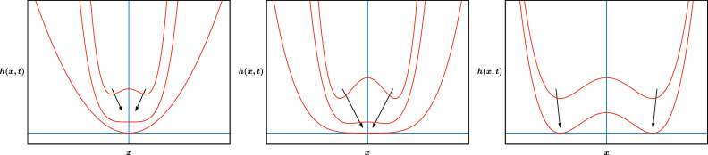 Figure 1
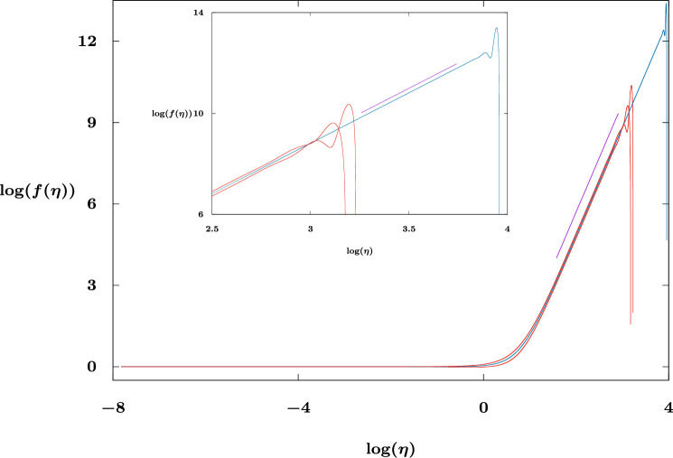 Figure 2
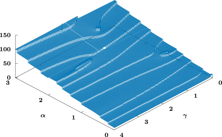 Figure 3
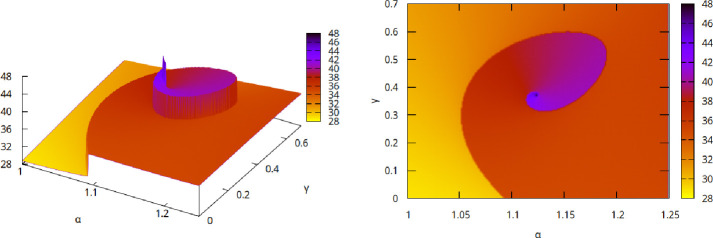 Figure 4
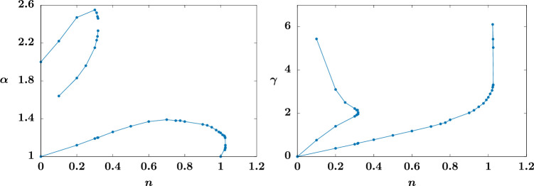 Figure 5
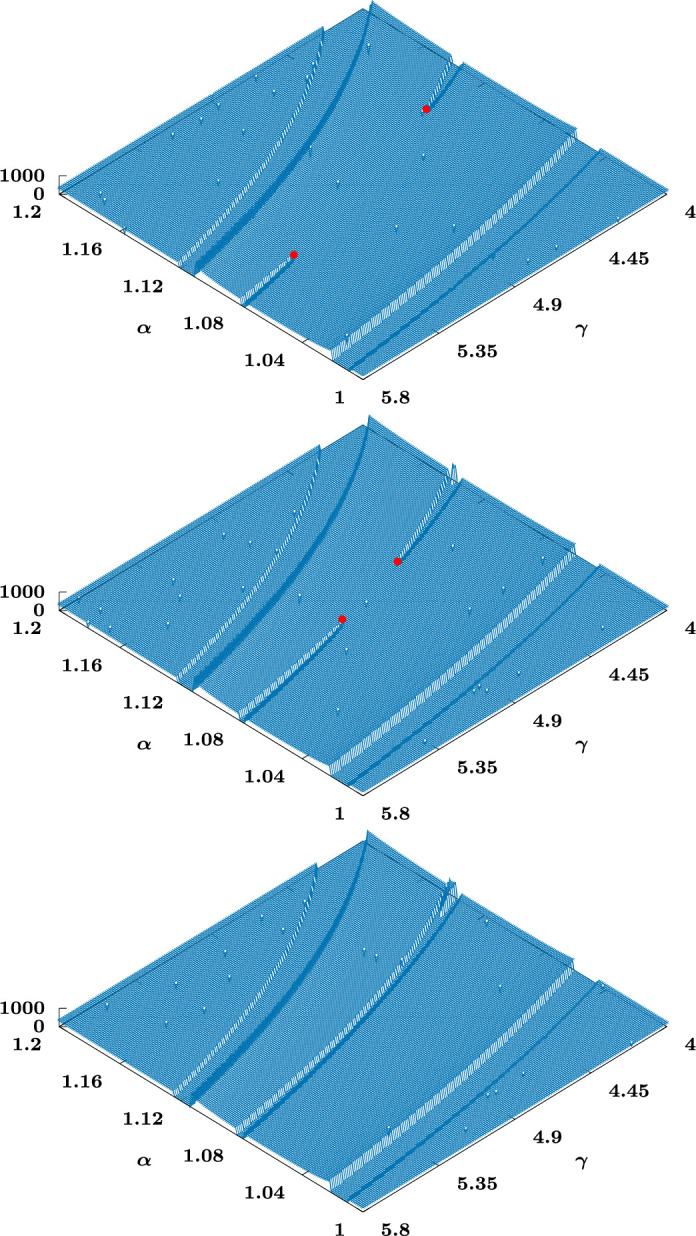 Figure 6
- —Royal Society Leverhulme Trust
- —Waseda Universityhttp://dx.doi.org/10.13039/501100004423
Peer Reviews
No public reviews on file for this paper yet. If you reviewed it on a platform where reviews are public (OpenReview, ICLR, NeurIPS, ICML), you can paste yours below so the community can read it here.
Videos
No videos yet. Explain this paper in a talk, walkthrough, or lecture? Add one.
Taxonomy
TopicsFluid Dynamics and Thin Films · Fluid Dynamics and Turbulent Flows · Theoretical and Computational Physics
Introduction
One of the emerging areas of mathematical modelling identified in [1] was the so-called thin-film equation (TFE)
for both its physical and its mathematical implications; see [2], for example, for further background and references. It has indeed been the case that such high-order parabolic equations have amply demonstrated their worth, with wide-ranging investigations pursued—we limit ourselves here to noting that early work includes [3–7]—but a large number of key questions remain open—we seek to shed significant light on one of the most important of these below.
The system of equation (1.1) arises in the surface-tension-driven spreading of a thin film of viscous (Newtonian) fluid over a planar substrate; in this context, the physically most significant values of the exponent are (no-slip on the substrate), (Navier-slip dominated) and (a slender thread in a Hele-Shaw cell). It is striking that each of these special values also plays an important role mathematically: most famously, is the main borderline case in terms of the motion of contact points (i.e. points separating regions with and ); and will play important roles in what follows. Other values with can be viewed as being associated with other slip laws (see appendix A), but the most direct physical interpretations of such cases are perhaps by similarly close analogy with a more general model for power-law fluids [8–11], whereby and correspond, respectively, to shear-thickening and shear-thinning flows with no slip (with corresponding equivalences holding either side of ). Both of the above (i.e. power-law slip and power-law fluids) lead to a doubly nonlinear generalization to equation (1.1) that is briefly discussed in appendix A.
The most prominent features of equation (1.1) are its degeneracy (i.e. the mobility vanishes at for ) and its high order; indeed, it exemplifies many of the difficulties that arise much more generally from these characteristics. The corresponding second-order case (the porous-medium equation, PME), , has been the subject of very extensive analysis (e.g. [12]); a key property of the PME is the presence of a comparison principle, implying in particular that at a minimum at which , so a positive solution cannot touch down to . Crucially, this is not the case for equation (1.1) and it is this possibility (having the important physical interpretation of film rupture) that we revisit below (e.g. [13] for an account of early work), an important open question being the upper value of the exponent for which rupture is possible.
Another area of very extensive current activity is that of non-local diffusion equations, and this provides a further perspective on equation (1.1) as an instinctive model problem. Thus, with a suitably scaled kernel , the non-local relationship
implies, on expanding in powers of for small ,
where is assumed bounded for . Then as the PME results from the first of equation (1.1) unless ; if also (typically because is even) then a scaled version of equation (1.1) arises when .
A tool widely used in studies of the PME that is applicable to the TFE is that of similarity solutions: equation (1.1) has two translation symmetries, and for arbitrary constants and , and two rescaling symmetries,
for arbitrary constants and . The symmetries of equation (1.2) imply the existence of a one-parameter ( ) family1 of similarity reductions
that will be central in what follows.
The rupture behaviour of equation (1.1) is notoriously complicated and we shall limit ourselves here to the symmetric case in which touchdown occurs at and (on appealing to the translation-invariance symmetries) with
with equation (1.2) providing a natural candidate for the behaviour as such a singularity develops, though it is far from the only relevant possibility, as we shall see. Aspects of what follows that are of much broader applicability include both (i) the role of symmetries and ‘second-kind’ similarity solutions (e.g. [14]) involving anomalous exponents ( in equation (1.3)), as well as of non-self-similar multiscale descriptions, and (ii) the significance of hierarchies of singular behaviour. We shall return to both of these issues in due course.
The linear case, n=0
This case is unusually revealing of the range of possibilities despite its linearity; moreover, its tractability provides a valuable starting point for the numerical investigations. That this case is perhaps unexpectedly simple to analyse owes as much to the fact that (exceptionally) has no special status—so the solution is analytic in both and at rupture—as to the TFE being linear when .
Since at , , with having a minimum at immediately beforehand (at least), we have as , that
where the are constants2 and successive terms are higher- and higher‐order even polynomials in , so generic touchdown behaviour has with3
and there are two singly non-generic cases (unstable to a single mode), namely, , with
and , , , with
Equation (2.2) is the second of a family of similarity solutions of the form equation (1.3), with for integer and , that are candidates for local descriptions of touchdown; the first of these is simply
the much more general role of which we shall come to shortly for . For odd these similarity solutions vanish at , so an additional term in the expansion (as in equations (2.1), (2.3) and (2.6)) is needed to determine as (conversely for even there is no contribution, etc.; such properties are unusual, but intrinsic to the current problem). The cases equation (2.1) and equation (2.3) are not of the class equation (1.3) and readily generalize to other , as we outline below; these are necessarily multiscale—thus equation (2.1) and (2.3) are, respectively, to be supplemented generically by
wherein the right-hand sides are subdominant to each of the terms on the left-hand sides and are of the form equation (1.3).
Interpretations of equations (2.2) and (2.3) are transparent in this context: equation (2.2) lies, for symmetric initial data with (say) a maximum at and a minimum in each of and , on the borderline between cases in which the three extrema merge before touchdown (so equation (2.1) ensues) and those in which touchdown occurs simultaneously at points in and (see figure 1 for a schematic); equation (2.3) involves touchdown followed immediately by lifting up again, and is thus the borderline between rupture via equation (2.1) and failure to touchdown (with reversing sign at , ) in the neighbourhood of : simple expressions such as
Generic (left and right) and non-generic (centre) touchdown scenarios. (Left) extrema merge before touchdown; (centre) extrema merge at touchdown; (right) separate touchdown points. Arrows indicate the direction of increasing t, successively lower curves corresponding to successively larger values of t.
serve to illustrate such behaviour, with , and , respectively, corresponding to this trichotomy. Such insights have more general implications—indeed, such transitions are not partial differential equation (PDE) specific, being a rather general feature of systems for which touchdown and lift off are possible (cf. [15]).
For completeness, we note that the second (multiscale) hierarchy has
for and that there are other possibilities as exemplified by , whereby
indeed, the general such form involves two positive integers and with
for , .
There is an alternative root to the same conclusions when equation (1.1) is posed as an initial value problem on the entire real line, which provides more details and hence is worth recording even though the methodology does not carry over to the nonlinear cases and may not be applicable to other initial boundary value problems for . Introducing the Fourier transform
and imposing even initial data
for some such that touchdown occurs at , we have
so that
where and
determine the coefficients of each of the polynomial similarity solutions in terms of the initial data. Since touchdown occurs at , holds in equation (2.7).
n>0: multiscale phenomena
The analysis of this section generalizes4 that of the previous one by using the exact solution
to equation (1.1) (where we have scaled so that ) as a starting point. Aspects of what follows have previously been established (e.g. [13]; it would not be appropriate here to review the extensive literature in the area) but our viewpoint differs, specifically in the way in which we regard equation (3.1) as a similarity solution of the form equation (1.3) with , and viewing the ‘outer’ scale (in the sense of matched-asymptotic expansions) as dictating the singular behaviour.
To set up this outer problem, we must first analyse the ‘inner’ one, in which the right-hand side of the TFE dominates, so that as
where as remains to be determined by matching, the final term in equation (3.2) having been matched into equation (3.1), which is the leading-order outer solution. Setting , the first correction term is then given by
for some function of integration . Hence, for
(we note that , and are all special cases with respect to equation (3.3), the significance of which will become clearer in due course), while for
Turning now to the outer scale, we set
and linearize to give
with matching into equations (3.2), (3.4), (3.5) determining boundary conditions on equation (3.6), namely,
the distinction being associated with the difference between equation (3.4) and equation (3.5). The associated eigenmodes take the form
and are to be determined as the non-trivial solutions to
subject to
and to
in both cases, the possible values of being the associated eigenvalues.
Determining the other possible contributions as reveals two exponentially growing expressions that are inadmissible (i.e. equation (3.11) amounts to two boundary conditions) and one exponentially decaying one: applying the Liouville–Green method to equation (3.10) requires that in the ansatz
satisfy
at leading order, so that
or
wherein only the real root equation (3.12) is admissible, with both of equation (3.13) being associated with oscillatory growth.
We now address the possible solutions to the linear problem equation (3.6) with equation (3.7) or equation (3.8) as , . For , the possibilities are given by immediate generalizations of the results for . The first two eigenmodes5
should be rejected: the former would dominate equation (3.1) for small , being associated with -translation invariance (i.e. with a different touchdown time), while the latter has already been absorbed into the choice of scaling in equation (3.1), reflecting the scaling invariance of equation (1.1). Turning to the remaining eigenmodes, which alongside equation (3.14) are expected to form a complete set in the traditional sense,6 the next two are given for (so that equation (3.7) holds) by
from which the general pattern should be clear; these modes are remarkable both in that those with , , have no terms, while those with omit terms, and in that the admissible exponentially decaying term (see equation (3.12)) as is entirely absent. These solutions should be viewed as second-kind similarity reductions of the form equation (3.9) of the linearized problem: that this family of solutions can be constructed explicitly, rather than only numerically, is associated with the sequence of eigenmodes generating a Taylor expansion in —see appendix A for additional comment and for a generalization for which such a construction is not possible.
The first of equation (3.15) with gives the generic form of touchdown, with following on matching. We must defer one of the two singly non-generic cases—with interpretations mirroring those for —to §4; that which generalizes equation (2.3) has , , with therefore resulting; plays no leading-order role in this scenario, but does lead to
which is generically the case.
The above computations closely parallel those for , but an additional check is needed, that is, that is subdominant to equation (3.1) as on the relevant scale, , requiring that (i.e. in equation (3.9) needs to be larger than the value associated with equation (3.1)). Thus, importantly, the first of equation (3.15) is admissible only for , becoming of the same scale as equation (3.1) at , which suggests the possibility that a similarity solution equation (1.3) distinct from equation (3.1) may then come into play, a possibility that we explore below. That the inner ( ) and outer ( ) scales would coincide for provides further evidence for such a possibility. Given the constraint that the other modes are all admissible.
Turning now to the regime, given equation (3.8) the modes with , , starting with the second of equation (3.15) remain applicable, but those with do not, being replaced by ones having of which the first two are
the first of these must be excluded for similar reasons to those noted above. Admissibility of these requires that , so those with remain legitimate, while for the constraint
must hold, so in particular the second of equation (3.16), which would otherwise represent the generic scenario, is not viable throughout , while equation (3.17) reveals that more and more of these modes become illegitimate as increases, all being lost at . The minimum height for is determined by matching into the final term of equation (3.5), whereby as
so that
The two most significant outcomes from the above analysis are that (i) touchdown is possible for any (we recall that is of specific physical interest), but does so only under more and more exceptional circumstances as increases, and (ii) there are possible bifurcations (to other solutions of the form equation (1.3)) at and for . We turn to the latter next.
n>0: similarity solutions
Two starting points for the analysis of similarity solutions of the form equation (1.3) that follows have been identified, namely, (i) by continuation from at 7 and (ii) via bifurcations at and , where . The latter are, in principle, amenable to weakly nonlinear analyses, but these seem unusually involved and we resort from the start to numerical approaches to the boundary value problem:
Similarly to equation (3.11), here equation (4.3) amounts to two boundary conditions, with two exponentially growing correction terms excluded. We note that is an (unknown) eigenvalue (i.e. equations (4.1)–(4.3) represent a nonlinear eigenvalue problem, cf. footnote 1). Our numerical approach (see §5) will adopt a shooting-problem set up from with
the former exploiting the scaling invariance of equation (4.1), with and both being shooting parameters.8
We next outline how we identify solutions to equations (4.1)–(4.3) numerically through the above shooting problem, the solution to which will generically reach zero at a finite value of , say, via9
when , wherein the presence of four arbitrary constants , , and confirms that this behaviour is generic. For special values of and , the solution will reach zero in a singly exceptional (three-parameter) way, with
for , with , and
for , with . The solutions that satisfy equations (4.5)–(4.7) for finite are inconsistent with equation (4.3),10 but those of the form equation (4.6) or equation (4.7) provide the cliffs in the simulations presented below, and hence will be significant in the identification of the desired connections (i.e. solutions that instead satisfy equation (4.3)): these connections are doubly exceptional, having two degrees of freedom (namely, the coefficients of and of the exponentially decaying term) as , consistent with there being two shooting parameters.
If we suppose , , furnishes a solution to equations (4.1)–(4.3) then for nearby values of the shooting parameters
we can set
and demonstrate, for as , that
wherein
and the constants , , and are independent of and and could be obtained numerically. Given its exponential growth, becomes of under the scaling
with , so setting
we obtain, at leading order in , the initial value problem11
The argument by which we identify the desired connections now proceeds in two distinct steps and is of an unusual type. First, for almost all the solution to equation (4.9) and equation (4.10) will hit zero in the form implied by equation (4.5), but for special curves in the plane equation (4.6) or (4.7) will apply instead. If we locate such an exceptional zero at , say, then on one side of such a curve the solution will hit zero near , while on the other side it will just fail to do so in this neighbourhood (this being the significance of equation (4.6) and (4.7) as a borderline case) and will instead do so at an distance further in (with increasing for an range of positive ); thus these curves will appear as vertical cliffs in surface plots in the plane of the location of the zeros of .
The second step in the argument then proceeds as follows. Introducing
expresses equation (4.10) in the form
and, setting , this becomes
so that depends upon and only through the combination (reflecting the translation invariance of equation (4.9)). Hence, if , lies on a cliff of the type referred to above, then for equation (4.9) and (4.10) the entire logarithmic spiral
will form the cliff over some range of . In consequence as , so a desired connection necessarily lies at the centre of such a spiral when lies in the relevant range.
Two related remarks about this analysis are in order.
(I) The result equation (4.11) is exact for equation (4.9) and (4.10), but only valid asymptotically close to a connection for the original problem equations (4.1), (4.2) and (4.4).(II) Both the logarithmic dependence of equation (4.8) upon and the spiral form equation (4.11) militate against the numerics fully uncovering the relevant details but, as we shall see, the above properties suffice for the current purpose.
Computations of the self-similar solutions
In this section, we provide numerical support for some of the conjectures made above, moreover determining numerically estimates of the values of and . We numerically solve equation (4.1) and (4.2) with equation (4.4) as a two-parameter shooting problem ( and in equation (4.4)) to identify the doubly exceptional solutions that satisfy equation (4.3) as .12 We present example solutions that demonstrate the effectiveness of the approach in figure 2 for , with and . The solutions with sit slightly on either side of the exact solution (with ) ; we include a line segment on the figure to indicate the far-field behaviour as . We note that the (red) curves in figure 2 (corresponding to ) have becoming zero well before the curve corresponding to . Furthermore, we note that the red curves separate from the blue curve in an opposite and oscillatory fashion, this being a consequence of the two exponentially growing oscillatory modes discussed above.
Log–log plots of f(η) versus η for n=0, α=1 with γ=±0.1 (red curves) and γ=0 (blue curve). The line segment has slope 4 (=α/β). The inset plot is an enlargement of the right-hand side of the larger plot.
Importantly, numerical errors for the solution eventually lead to the growing modes again dominating and as a consequence it can be difficult, even for the linear case, , to distinguish the doubly exceptional solutions. However, as indicated in figure 2, we expect the numerically obtained critical solutions to be the ones that locally (in parameter space) touch down (i.e. have ) at the largest value of and this provides a robust measure for finding such solutions for also. Our results are therefore primarily presented as parameter surveys of the value of corresponding to the first zero of ; the sought after exceptional solutions appear (within numerical resolution) at the centre of logarithmic spirals (see §4).
Figure 3 shows an example parameter survey for . Notably, three doubly exceptional solutions (spiral centres) can be observed, these being the continuations into of the (rescaled13) exact solutions (i) , , (ii) , and (iii) , (we omit the figure for ). We also include a close-up view of the spiral structure of the branch (i) for in figure 4, wherein it can be observed that attains a maximum as the centre of the spiral is reached.
Surface plot for n=0.2, the surface height corresponding to η0 for f(η0)=0, illustrating the spirals corresponding to the solution branches starting from α=1 (right), 3/2 (left) and 2 (top) at n=0.
Close-up view of the spiral corresponding to the solution branch starting from α=1 at n=0 from figure 3 (for n=0.2). (Left) side-view, (right) map-view. The darkening colours indicate how η0 attains a maximum as the centre of the spiral is reached.
We record the locations in parameter space of the exceptional solutions as varies in figure 5. In the left-hand figure, the top branch corresponds to that starting from when . At , this branch annihilates with that coming from at . In the right-hand figure, the lower branch (corresponding to the one starting from at ) folds back just beyond before having as . In other words, for a value of close to, but above, one, a fold arises as solutions on separate branches come together, at ; given the small range of beyond on which the fold occurs, the numerical simulations here are particularly delicate. We include figure 6 to illustrate how the two branches approach each and coalesce as the fold occurs.
Plots of α (left) and γ (right) against n showing the location of the centre of the spirals located in (α,γ) parameter space (corresponding to doubly exceptional solutions). The highest branch in the right-hand pane corresponds to the middle one on the left, having γ→∞ as n→0+ (the α=3/2 solution at n=0 having no η2 contribution).
Surface plot for (upper figure) n=1.025, (centre figure) n=1.026 and (lower figure) n=1.027, showing the solution that originates from α=1 at n=0 (upper tip) and the solution that has α=1 at n=1 (lower tip). The surface heights correspond to η0 for f(η0)=0. The dots are intended to be indicative of the cliff-end tips as they approach each other, with coalescence having occurred by n=1.027.
The main conclusions from the very extensive numerical study summarized above, which we believe has identified for the first time the role in touchdown behaviour of similarity solutions satisfying equations (4.1)–(4.3), are the following.
(a) The first three similarity solutions identified for can all be continued into , though the second and third annihilate at a fold at . The first, though, seems to persist until just above , providing the continuation of the singly degenerate solution equation (2.2) the significance of which was noted in §2. The continuation of higher modes would require further numerical study.(b) The fact that the first branch extends up to is the single most significant result: the numerical evidence is that a fold occurs there with the solution branch that emerges from , ; for below the value at the fold this branch is expected to be generic in the current context, so extends the class of stable touchdown solutions to the symmetric problem to slightly above . While the above value of is sufficiently close to one that we cannot exclude this conclusion being the result of numerical inaccuracies, the presence in figure 6 of two terminating cliffs (with termination points that move closer together as the putative fold is approached) provides good qualitative evidence for their being two distinct, but neighbouring, solutions in the relevant range of . In any case, the implications of the singly unstable solution branch noted in the context of equation (2.2) makes its presence up to at least noteworthy.(c) No solutions to equations (4.1)–(4.3) that bifurcate off at have been detected, the implication being that the bifurcations are plausibly to similarity solutions describing other types of singular behaviour (associated with contact-point motion). Such matters warrant further investigation.
Discussion
We start with some comments specific to the above analysis, before turning to some more general matters. The most significant result above is that touchdown scenarios are available up to, but we believe not including, , but in the symmetric case rupture seems to be possible generically only to slightly above , both classes of analyses undertaken above being needed to establish this claim. That non-generic scenarios are available for larger is mathematically significant, but such phenomena would naturally be hard to capture numerically from time-dependent solutions and would compound the challenges associated with rigorous studies. Our results are based on a combination of formal and numerical approaches and are accordingly not in that sense conclusive (including because we have not addressed asymmetric cases, in which other balances are known to be relevant); nevertheless, the evidence they provide for new touchdown scenarios up to, but not beyond, would seem to be significant given both the long-standing open nature of the question and the physical significance of (there is additional evidence that should hold in the case of equation (1.3), reinforcing this claim of criticality). With regard to , we should note that the combination of nonlinearities
is commonly adopted in applications, with the dimensionless slip parameter often small— nevertheless, in the limit with which we are concerned, the term dominates the right-hand side even for small .
Criticality is indeed a common theme in the above, with the presence of a number of distinct regimes in the exponent being of particular significance. Analysis of the critical cases (notably , and ) is, as usual, particularly delicate and has not been undertaken here. While the analyses above establish local spatial profiles at touchdown, we have also not outlined the resulting post-touchdown evolution, though much of this can be gleaned from [16].
The following more general issues seem worth highlighting. Self-similarity and other symmetry arguments are central to progress in such applications; moreover, the results above are in fact of near-direct broader relevance to other singular phenomena in the TFE. Entire hierarchies of the type described above necessarily arise in such contexts, for reasons implicit in the discussion of the singly non-generic cases in §2. A combination of various analytical and numerical approaches, as exploited above, is of very broad applicability, the interplay between them being particularly fruitful. A variety of analytical arguments were needed to characterize the possibilities in full, and it is striking that a number of the most instructive ones are elementary, allowing us to elaborate many of their details—a further example of this type, which also revisits the issue of critical exponents, relates to the possible local behaviours of in equation (3.6), namely, time-dependent multiples of
the comparison of the last of these with the other three immediately identifying , and as critical.
As is typical of such studies, the formal and numerical arguments could provide the basis for subsequent rigorous approaches, involving analysis either of the (high-dimensional) phase space of the ODE (4.1) or of the full (time-dependent) PDE (1.1). Each would be valuable and each challenging; their combination would be particularly potent.
A number of natural extensions suggest themselves. The critical exponents could change in higher dimensions (the two-dimensional generalization being the only physically meaningful one in the thin-film context), though a preliminary analysis of the radially symmetric case suggests that surprisingly little changes (including the upper bound of ); non-radially symmetric cases are, unsurprisingly, much more involved, though aspects seem to be accessible to methods closely related to those above (most notably, the steady state solution equation (3.1) generalizes in two dimensions to for arbitrary positive constants and , allowing non-radial singularities to be identified). The inclusion of additional physics, such as con/disjoining pressure terms and stochastic effects (e.g. [17]) seems likely to have more dramatic implications for criticality and goes beyond the scope of the current study.
In summary, we have identified new touchdown scenarios relating to a long-standing open problem, with the critical value of the exponent in equation (1.1) deserving emphasis. We have applied a combination of analytical and numerical arguments, with intuition as an invaluable adjunct, in deriving two classes of second-kind self-similar behaviour: first, similarity solutions to the linearized problem equations (3.6), (3.9), are the key ingredients in §3; second, and most notable, those of the full PDE (1.1), satisfying equations (4.1)–(4.3), have been explored in §§4 and 5–to the best of our knowledge the role of such solutions in touchdown has not previously been identified, though the regimes in which they are present are perhaps surprisingly limited. The story is certainly not yet over, with intriguing issues remaining—open questions have been noted above, and other approaches would be needed to rule in or out dynamics more exotic than the power-law dependencies uncovered above—but it seems worth highlighting that considerable insight can be obtained by perhaps deceptively simple-looking arguments.
The reference list from the paper itself. Each links out to its DOI / PubMed record.
- 1King JR. 2000 Emerging areas of mathematical modelling. Phil. Trans. R. Soc. Lond. A 358, 3–19. (10.1098/rsta.2000.0516) · doi ↗
- 2Bertozzi A, Bowen M. 2002 Thin film dynamics: theory and applications. In Modern methods in scientific computing and applications (eds A Bourlioux, MJ Gander, G Sabidussi). Dordecht, The Netherlands: Springer. (10.1007/978-94-010-0510-4_2) · doi ↗
- 3Smyth NF, Hill JM. 1988 High-order nonlinear diffusion. IMA J. Appl. Math. 40, 73–86. (10.1093/imamat/40.2.73) · doi ↗
- 4Bernis F, Friedman A. 1990 Higher order nonlinear degenerate parabolic equations. J. Differ. Equ. 83, 179–206. (10.1016/0022-0396(90)90074-Y) · doi ↗
- 5Boatto S, Kadanoff LP, Olla P. 1993 Traveling-wave solutions to thin-film equations. Phys. Rev. E 48, 4423–4431. (10.1103/Phys Rev E.48.4423)9961123 · doi ↗ · pubmed ↗
- 6Almgren R, Bertozzi A, Brenner MP. 1996 Stable and unstable singularities in the unforced Hele-Shaw cell. Phys. Fluids 8, 1356–1370. (10.1063/1.868915) · doi ↗
- 7Myers TG. 1998 Thin films with high surface tension. SIAM Rev. 40, 441–462. (10.1137/s 003614459529284 x) · doi ↗
- 8King JR. 2001 Two generalisations of the thin film equation. Math. Comput. Model. 34, 737–756. (10.1016/S 0895-7177(01)00095-4) · doi ↗