Water beetle networks differences and migration between natural lakes and post-exploitation water bodies
Joanna Pakulnicka, Marek Kruk

TL;DR
This study explores beetle community networks in natural lakes and post-exploitation water bodies to understand migration patterns and ecological stability.
Contribution
The paper introduces a novel approach combining network analysis and machine learning to assess beetle migration and ecological network stability in different water bodies.
Findings
Ecological networks in eutrophic lakes and clay ponds show the highest network density.
Beetle species like argilophiles in gravel pits show a stronger affinity to dystrophic lakes.
Rheophiles in clay pits primarily originate from mesotrophic lakes, contributing to functional connectivity.
Abstract
Water deficits are a serious problem around the world, which also affects young landscapes, where lakes are most abundant. This poses a threat to many habitats and biological diversity found here. The relationships between species in the ecological networks of lakes at different stages of development and in nearby post-exploitation water bodies remain poorly understood. To better understand the functioning of beetle communities in different ecosystems, we created five network models that we subjected to graph analysis. By analysing the general attributes of the network (number of neighbours, shortest path, characteristic path length, clustering coefficient, network centralisation, network density and network heterogeneity) and those related to the nodes (NCC—Node Closeness Centrality, NBC—Node Betweenness Centrality, NDC—Node Degree Centrality) and to the edges (EBC—Edge Betweenness…
Genes, proteins, chemicals, diseases, species, mutations and cell lines named across the full text — each resolved to its canonical identifier and authoritative record.
Click any figure to enlarge with its caption.
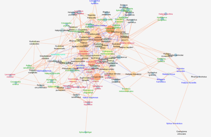 Figure 1
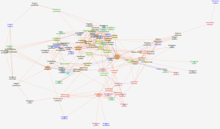 Figure 2
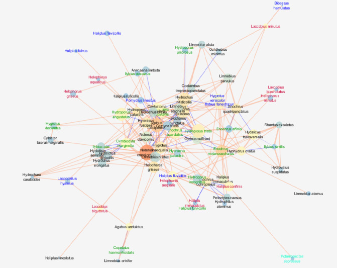 Figure 3
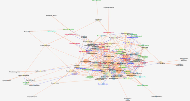 Figure 4
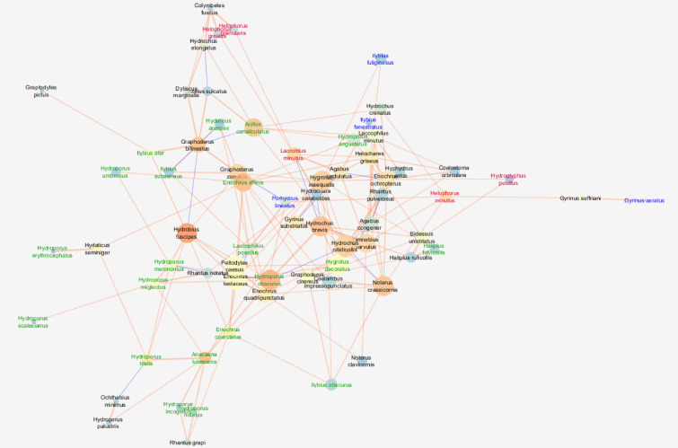 Figure 5
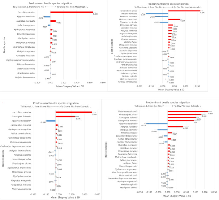 Figure 6
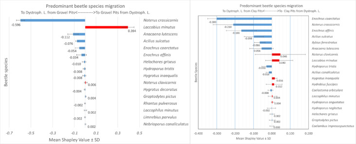 Figure 6
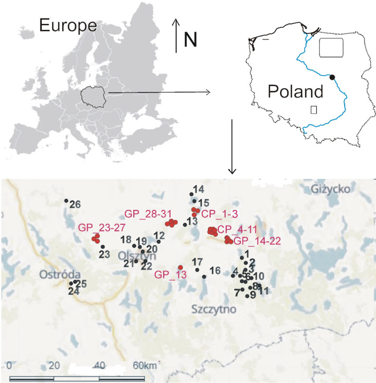 Figure 7
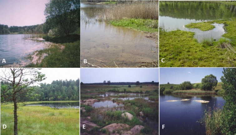 Figure 8
Peer Reviews
No public reviews on file for this paper yet. If you reviewed it on a platform where reviews are public (OpenReview, ICLR, NeurIPS, ICML), you can paste yours below so the community can read it here.
Videos
No videos yet. Explain this paper in a talk, walkthrough, or lecture? Add one.
Taxonomy
TopicsSpecies Distribution and Climate Change · Freshwater macroinvertebrate diversity and ecology · Forest Ecology and Biodiversity Studies
Introduction
One of the goals of biocoenosis ecology is to identify the mechanisms that determine patterns of species richness^1–4^. Many ecologists point to the dynamic nature of biocenoses based on dispersal, i.e. the movement of organisms between available habitats, which is the result of both natural changes and anthropogenic pressures across entire landscapes^3–7^. This is in line with metapopulation theory, which has been intensively developed in recent years^8–12^. According to this theory, the structure and functioning of biocenoses are based on complex interactions between organisms that form ecological networks^10,15–18^. However, the problem of insufficient recognition of the detailed structure and functioning of networks (their attributes) between different species affects many environments, including particularly sensitive ecosystems such as freshwaters, especially lakes^5,6^.
Huge water deficits are a serious problem around the world, which also affect young post–glacial landscapes, typical of northern and central Europe, including Poland. The ecological landscapes are higher-level ecological systems composed of many ecosystems that are interconnected through the interaction of abiotic factors and biotic relationships between species^19,20^. One of the potential biotic interactions among species is competition, which in the course of evolution shapes the structure of biotic networks and trophic relationships typical of a given system – a network of trophic chains that ensures the transfer of energy through subsequent trophic levels^21^. Ecosystems are open systems, as food chains extend beyond their boundaries thanks to the migration of organisms. One of the biocenotic principles is the fact that all species enter into biocenotic relationships and are therefore all important for the stabilisation of the ecosystem. Migrations between ecosystems enable the maintenance of biodiversity and thus guarantee the stabilisation of the ecological landscape^19,20^. This is particularly important because ecological systems are dynamic and subject to changes that accelerate anthropogenic activities^22^.
Natural lakes are an essential element of the young glacial landscapes of north–central Europe, which were formed during the recession of the last, fourth ice age, the so-called Vistula Glaciation^23^. In Europe, the total number of natural lakes with an area of more than 1 ha is over 500,000. Poland has around 7000 lakes over 1 ha in area each, which corresponds to 1.42% of all lakes in Europe. They are mainly located in the Pomeranian and Masurian Lake District^24^. Despite their common history of formation, they are in different stages of ecological succession, at the end of which they will disappear completely. According to Choiński et al.^24^, only 40% of all formed lakes are still preserved, and their average age (around 2,000 years) proves their episodic character at the geological scale. The evolution of lakes essentially follows two different directions: according to the harmonic series, which is linked to the successive increase in the fertility of lakes from oligo-, meso-^25^, and according to the disharmonic series, which is linked to the evolution from dystrophic lakes in the forest to polyhumic lakes and then to peat bogs^25,26^. Although the final fate of lakes is fixed and the pace of their evolution depends on many natural factors such as climate, location and morphometry, this process is additionally accelerated by human pressures, e.g. agriculture, livestock, forestry, hydro-engineering practises, deforestation and peat mining^27–32^. For this reason, the Water Framework Directive (WFD), which constitutes the basis for developing a protection and restoration system aquatic environment, requires that EU Member States should aim to achieve good status for all surface waters and groundwaters^33^.
A side effect of anthropogenic pressure is the appearance of artificial water bodies in the landscape, which are created by filling pits with water after excavation^34–37^. They complement the natural hydrographic network and form extensive anthropogenic lake areas in many areas^38^. In the lowlands of Poland, there are a particularly large number of water bodies created by the exploitation of mineral resources such as sand, gravel or clay, which are needed for the construction of infrastructure^34,35^.
The deterioration of lake water quality, the disappearance of some habitats and, over time, of entire lakes, leads to a deterioration of fauna, a decline in local biodiversity and, in particular, the disappearance of the most sensitive species^27,31,39–41^. The most endangered part of the lake, which remains under pressure from strong external factors, is the littoral zone^31,42^. This is where the greatest species richness of macroinvertebrates is recorded, especially specialised species that are more sensitive to changes in the environment. This is a prerequisite for the use of macroinvertebrates in the monitoring of aquatic ecosystems, which is in line with the recommendations of the Water Framework Directive^43–46^. Taking into account all the consequences resulting from the transformation and disappearance of lake ecosystems, anthropogenic water bodies are becoming an important element of the landscape^34,35,37^. They take over the function of ecologically young lake ecosystems and become a substitute habitat, a kind of refuge into which the lake fauna invades, especially the most sensitive and endangered species^21,47–49^.
In the extensive literature on the entomofauna of aquatic habitats, there are many papers on aquatic beetles inhabiting lakes, but knowledge of this group of insects in anthropogenic water bodies is very scarce^35,50–53^. Therefore, little is known about the structure and functioning of ecological networks in them, which are characterised by trophic interactions (food chain) between species, which in turn are fragments of complex food webs^5,6,54,55^. Little is known about the mechanisms of migration (intensity and direction) of aquatic organisms between different ecosystems that shape the structures of fauna in supra–ecosystemic systems at the landscape scale^21,56–59^. Most of the available studies concern river valleys^60–66^. Only a few of these studies concern particularly well-migrating organisms, i.e. water beetles^67–72^. Many hydrobiologists now refer to water beetles as bioindicators of both the ecological status of water bodies^45,46,57,73–75^ and the biodiversity of the entire macrobenthos of freshwater ecosystems^46,73,76^. Beetles are usually very abundant in various aquatic environments. At the same time, they exhibit great species, ecological and functional diversity. As adults, they show high mobility, which allows them to respond quickly to environmental stress and even migrate over long distances^36,56,57–59^. Migrations between ecosystems are important for maintaining regional biodiversity, which influences the maintenance of dynamic equilibrium in the ecological landscape^22,41^.
In this context, it is important to recognise the mechanisms of beetle migration, especially between disappearing lakes and relatively young anthropogenic water bodies. These are complex problems that require the collection of many field observations and tools that allow a difficult interpretation of the complex relationships between species that occur in multidimensional ecological systems, as emphasised by, among others^55,77–81^. In recent years, modelling based on machine learning algorithms has become a useful research tool in the ecology of aquatic ecosystems. Høye et al.^82^ pointed out the need for a broader application of machine learning methods in the study of insect communities. The use of modelling based on boosting and SHAP algorithms to analyse the interactions of aquatic species has been applied in the study of their properties to assess water quality in microbiological studies in coastal waters^83,84^, in the analysis of the response of lagoon water properties to weather dynamics^81^ or in the analysis of the biocenotic effects of climate warming on the zooplankton community^85^. In the last two articles, the applied methods of the explainable machine learning of XGBoost–SHAP and their effectiveness in ecological research are discussed in detail. Their evaluation enables a more thorough analysis of the structures of various biocenoses, their formation and functioning under changing environmental conditions, as well as the assessment of the role of individual species in the cohesion, i.e. the durability of the analysed ecological networks^55,77–81^. Machine learning is a method to support ecosystem management^85,86^. This includes predicting the direction of adaptation of biocenotic systems to changing environmental conditions, e.g. climatic or anthropogenic^78,87,88^ and can also help in finding ways to restore already degraded habitats^5,6^.
The aim of our research was: (1) to compare the characteristics of the networks of species in beetle communities in mesotrophic, eutrophic and dystrophic lakes and anthropogenic water bodies—clay pits and gravel pits, (2) to determine the importance of individual species and the mutual connections between them in these networks, (3) to determine the role of distinctive and functional elements in the structure of the network in specific types of water bodies, (4) to identify species that show significant migration tendencies from specific water body types to clay and gravel pits and from anthropogenic water bodies to specific water body types, and to determine the species range and intensity of these migrations, (5) to specify species that are important for functional uniformity in landscapes.
Results
General characteristics of the collected material
In total, we collected 19,923 beetles representing 167 species with a total wet biomass of 367,119.81 mg (Tables 1, S1). The species diversity in the samples collected in in different types of water bodies studied was 72–114, with only 25 species occurring in all types of water bodies. We found the largest number of species in eutrophic lakes, where we also collected the most beetles. The least species-rich material came from dystrophic lakes. The fewest beetles were found in mesotrophic lakes.
Table 1. General characteristics of the material. N abundance, S number of species, \documentclass[12pt]{minimal} \usepackage{amsmath} \usepackage{wasysym} \usepackage{amsfonts} \usepackage{amssymb} \usepackage{amsbsy} \usepackage{mathrsfs} \usepackage{upgreek} \setlength{\oddsidemargin}{-69pt} \begin{document}$$\:\stackrel{-}{\text{x}}$$\end{document} mean, SD standard deviation, n number of samples.ParametersClay pits (n = 229)Gravel pits (n = 243)Mesotrophic lakes (n = 264)Eutrophic lakes (n = 260)Dystrophic lakes (n = 100)Total (1096)Abundance2974515013018514198419,923Min–max4–64113–108759–402140–58385–724 \documentclass[12pt]{minimal} \usepackage{amsmath} \usepackage{wasysym} \usepackage{amsfonts} \usepackage{amssymb} \usepackage{amsbsy} \usepackage{mathrsfs} \usepackage{upgreek} \setlength{\oddsidemargin}{-69pt} \begin{document}$$\:\stackrel{-}{\text{x}}\:$$\end{document} ± SD198.3 ± 178.1171.7 ± 221.1260.2 ± 154.91419 ± 2236.7132.3 ± 188.8Number of species1001068611472167Min–max2–532–4214–4822–703–343–114Total biomass (mg)64,196.3176,989.6549,873.85116,510.2659,549.74367,119.81Ecological groups—N, (S)Eurybionts (%)1927 (54)(64.79)833 (52)(16.17)575 (46)(44.20)5119 (63)(60.12)1020 (40)(51.41)9474 (89)Tyrphophiles (%)282 (23)(9.48)170 (23)(3.30)105 (16)(8.07)162 (22)(1.90)884 (22)(44.56)1603 (37)Argilophiles (%)343 (13)(11.53)4080 (19)(79.22)145 (9)(11.14)628 (14)(7.38)33 (8)(1.66)5229 (25)Rheophiles (%)406 (8)(13.65)66 (10)(1.28)473 (13)(36.36)2597 (12)(30.50)47 (4)(2.37)3589 (16)Rheobionts (%)16 (1) (0.54)1 (1)(0.02)3 (1)(0.23)8 (3)(0.09)0 (0)(0.0)28 (5)
The species richness found in the analysed water body types differed significantly (Kruskal–Wallis test: H(4,N = 71) = 11.34, p = 0.02 (Table 2). We also found significant differences in the number of beetles collected (Kruskal–Wallis test: H(4,N = 71) = 19.49, p = 0.0006). Statistically significant differences between the types of water bodies tested (p-value for multiple comparisons) are shown in Table 2.
Table 2. Differences between parameters in the analyzed types of water bodies. Results of ANOVA Kruskal – Wallis test: H – (statistics), df – degree of freedom, p – p value, N – abundance, S – number of species.ParameterHdf p Post–hoc (p)Abundance (N)11.344, N = 710.02Dystrophic–eutrophic (0.03)Numberof species (S)19.494, N = 710.0006Dystrophic–eutrophic (0.02)Eutrophic–gravel pits (0.009)Biomass15.674, N = 710.005Dystrophic–eutrophic (0.03)Eutrophic–gravel pits (0.001)Ecological groups (N, S)Eurybionts22.284, N = 710.0002Clay pits–gravel pits (0.02)Eutrophic–gravel pits (0.001)21.254, N = 710.0003Clay pits–gravel pits (0.02)Tyrphophiles16.134, N = 710.02Dystrophic–gravel pits (0.02)14.044, N = 710.007Eutrophic–gravel pits (0.046)Argilophiles29.984, N = 710.00001Dystrophic–gravel pits (0.0001)19.264, N = 710,0007Fystrophic–gravel pits (0.0002)Rheophiles30.114, N = 710.00001Dystrophic–eutrophic (0.0001)Dystrophic–mesotrophic (0.01)Eutrophic–gravel pits (0.004)Gravel pits–mesotrophic (0.005)30.574, N = 710.0001Dystrophic–eutrophic (0.0006)Dystrophic–mesotrophic (0.005)Eutrophic–gravel pits (0.0007)Gravel pits–mesotrophic (0.007)Rheobionts0.04, N = 711.0–
The most numerous species in the collected material were: Noterus crassicornis (16.31%), Laccobius minutus (11.47%), Anacaena lutescens (17.1%), Scarodytes halensis (10.11%), followed by Haliplus immaculatus (8.04%), Haliplus flavicollis (7.95%), Hygrotus versicolor (3.82%) and A. lutescens (3.21%). The species with the highest individual biomass were: Cybister lateralimarginalis, Dytiscus dimidiatus, D. marginalis, D. circumcinctus and Hydrophilus aterrimus. The individual water types were characterised by different numbers of the most numerous species but were always dominated by Noterus crassicornis and L. minutus (Table S1). The core of the fauna was formed by eurybionts (39.52%), which also exhibited the greatest species diversity in the entire material (86 species). A significantly lower species richness was observed in the tyrphophiles (37) and argilophiles (25). Argilophiles (24.2% of the total material) and rheophiles (18.01%) were of great quantitative importance (Table 1). The distinguished ecological groups contributed differently to the fauna in the analysed types of water bodies. Eurybionts were of greatest quantitative and qualitative importance in eutrophic lakes and clay pits. Rheophiles, on the other hand, were most numerous in eutrophic, mesotrophic lakes and clay pits, while argilophiles were found in gravel pits and tyrphophiles in dystrophic lakes. (Table 1). Significant statistical differences between the analysed environments (p-value for multiple comparisons) are listed in Table 2.
Network structure
The analysed network in clay pits was characterised by a moderate cohesion metric (clustering coefficient = 0.349), a density metric (0.079) and a centrality coefficient (centralisation) (0.113). At the same time, the highest values are for the number of nodes (species) (101), the average number of neighbours (7.901) per species (node), i.e. the number of interspecific interactions, as well as the values of the parameters describing the communication pathways between the taxa. This means the highest number of direct and indirect connections between species. In these waters, the shortest paths (10100) were found, indicating the highest number of highest correlations between species in the network, as well as a relatively high value of the so–called characteristic path length (3.718), indicating the presence of taxa communicating with the highest number of species (Fig. 1; Table 3).
Fig. 1. Network of correlations between beetle species in clay pits with node closeness centrality (NCC), node betweenness centrality (NBC) and correlation coefficient (R). Node size is proportional to the NCC measure; node colour from blue (dark) to orange (light) is proportional to the NBC measure; edge thickness is proportional to the correlation coefficient R. Sign of the relationship: a light orange edge represents positive relationships between nodes, while a dark blue edge represents negative relationships. The font colour means: red—argilophiles, blue—rheophiles, light green—rheobionts, dark green—tyrphophiles, black—eurybionts. The graph was generated using the Metscape application in the Cytoscape 3.7.2 package, https://cytoscape.org.
Table 3. General attributes of the water beetles network in compared regions.AtributeHabitatsClay pitsGravel pitsMesotropic lakesEutrophic lakesDystrophic lakesClustering coefcient0.3490.4080.3650.3340.294Network centralization0.1130.1010.2200.1930.076Shortest paths10,1008556540210,3024556Characteristic path length3.7182.9652.6702.6873.109Average number of neighbours7.9016.8826.3788.8435.029Number of nodes101937410268Network density0.0790.0750.0870.0800.075Network heterogeneity0.5940.5580.7270.6430.499
The network of interspecific interactions observed in the gravel pits was characterised by the highest cohesion metric (clustering coefficient = 0.408), while the network density was the lowest (0.075). The other attributes describing the networks had moderate values (Fig. 2).
Fig. 2. Network of correlations between beetle species in gravel pits with node closeness centrality (NCC), node betweenness centrality (NBC) and correlation coefficient (R). See the legend and explanations in Fig. 1 (clay pits). The graph was generated using the Metscape application in the Cytoscape 3.7.2 package, https://cytoscape.org.
The network observed in mesotrophic lakes was characterised by a relatively high cohesion metric (clustering coefficient = 0.365), while the centrality coefficient (centralisation) (0.220) and density metric (0.087) were the highest. It was also characterised by the highest fragmentation, as indicated by the highest value of the network heterogeneity parameter (0.727) (Fig. 3; Table 3).
Fig. 3. Network of correlations between beetle species in mesotrophic lakes with node closeness centrality (NCC), node betweenness centrality (NBC) and correlation coefficient (R). See the legend and explanations in Fig. 1 (clay pits). The graph was generated using the Metscape application in the Cytoscape 3.7.2 package, https://cytoscape.org.
The analysed network in eutrophic lakes was characterised by a moderate cohesion metric (clustering coefficient = 0.334) and density metric (0.079) as well as a relatively high centrality coefficient (centralisation) (0.193). At the same time, the highest values are for the number of nodes (species) (102), the average number of neighbours (8,843) per species (node), i.e. the number of interspecific interactions, and the values of the parameters describing the communication pathways between the taxa. In these lakes, the shortest paths (10302) were found, indicating the highest number of the highest correlations between species in the network, as well as a relatively high value of the so–called characteristic path length (2.687), indicating the presence of taxa communicating with the highest number of species (Fig. 4; Table 3).
Fig. 4. Network of correlations between beetle species in eutrophic lakes with node closeness centrality (NCC), node betweenness centrality (NBC) and correlation coefficient (R). See the legend and explanations in Fig. 1 (clay pits). The graph was generated using the Metscape application in the Cytoscape 3.7.2 package, https://cytoscape.org.
The lowest cohesion and the lowest density characterise the network in dystrophic lakes. This is confirmed by the values for clustering (0.294) and density (0.075) as well as centralisation (0.076). The network also had the lowest values for the average number of neighbours (5.029) per species (node) and the number of shortest paths (4556). At the same time, the presence of taxa communicating with the largest number of species was the highest among the five analysed networks, as shown by the value of the characteristic path length (5.029) (Fig. 5; Table 3).
Fig. 5. Network of correlations between beetle species in dystrophic lakes with node closeness centrality (NCC), node betweenness centrality (NBC) and correlation coefficient (R). See the legend and explanations in Fig. 1 (clay pits). The graph was generated using the Metscape application in the Cytoscape 3.7.2 package, https://cytoscape.org.
Interspecific relationships in water beetles networks
An important measure of interspecific relationships is node degree centrality (NDC), which describes the number of direct connections with a particular taxon (node) (Table 4). The highest NDC values were found in eutrophic lakes for Hydrobius fuscipes (28), Haliplus confinis (26), H. fluviatilis (19) and Agabus undulatus (10). The maximum NDC values were lower in the other habitats. In mesotrophic lakes they were observed for Noterus crassicornis (22) as well as Agabus fuscipennis (16), Hydroporus tristis (15) and Enochrus melanocephalus (15), in clay pits – for H. neglectus (19), Noterus crassicornis (18), N. clavicornis (18), Enochrus isotae (18) and Helophorus minutus (16), in gravel pits – for Agabus undulatus, Hygrotus decoratus and Hydroporus nigrita (16), as well as for Hygrotus inaequalis and H. neglectus (15). The lowest NDC values were determined in dystrophic lakes for N. crassicornis (10), as well as for H. fuscipes (9), Enochrus quadripunctatus, E. affinis, Hygrotus decoratus (8) and A. lutescens (7) (Table 4).
Table 4. Water beetle species with the highest net attribute. NCC node closeness centrality, NBC node betweenness centrality, NDC node degree centrality. The most numerous species.SpeciesClay pitsGravel pitsMesotrophic lakesEutrophic lakesDystrophic lakesNBC0–0.08NCC0.22–0.48NDC1–19NBC0–0.14NCC0.17–0.45NDC1–161NBC0–0.22NCC0.25–0.52NDC1–22NBC0–0.09NCC0.22–0.51NDC1–28NBC0–0.12NCC0.20–0.41NDC1–10 Hydroporus neglectus 0.080.4819 Noterus crassicornis 0.050.46190.220.52220.060.46200.090.4010 Rhantus grapi 0.040.4617 Agabus undulatus 0.040.46160.060.4520 Noterus clavicornis 0.060.46180.100.4115 Helophorus minutus 0.050.4616 Hydroporus erythrocephalus 0.020.46130.040.4315 Coelambus impressopunctatus 0.040.45160.060.4216 Cercyon tristis 0.070.4513 Enochrus isotae 0.050.4518 Laccobius atrocephalus 0.050.4512 Hygrotus inaequalis 0.030.45160.050.45100.080.4010 Graptodytes pictus 0.040.4411 Scarodytes halensis 0,020.4011 Hydrobius fuscipes 0.040.44140.070.43140.090.51280.120.409 Laccobius minutus* 0.040.46130.030.3340.070.367 Anacaena lutescens* 0.040.44160.010.3660.050.46110.090.367 Hydroporus nigrita 0.140.4515 Hydrochus ignicollis 0.090.4415 Haliplus ruficollis 0.040.4413 Hygrotus decoratus 0.060.42160.030.408 Enochrus quadripunctatus 0.060.4213 Ochthebius minimus 0.060.4110 Hydroporus angustatus 0.060.41120.050.4712 Enochrus affinis 0.020.40120.070.418 Agabus fuscipennis 0.120.4916 Hydroporus tristis 0.050.4915 Enochrus testaceus 0.050.4914 Enochrus melanocephalus 0.110.4515 Enochrus coarctatus 0.040.4713 Hydrochus nitidicollis 0.070.48160.070.418 Coelostoma orbiculare 0.030.4514 Haliplus flavicollis* 00.3310.030.4415 Haliplus fluviatilis 0.010.3050.030.4180.100,519 Haliplus fulvus 0.010.32400.301 Haliplus confinis 0.040.4250.050.4926 Haliplus immaculatus 0.020.4060.010.4314 Hygrotus versicolor* 0.020.4060.0050.377 Ilybius fenestratus 0.020.2830.050.4380.020.471300.261 Bidessus hamulatus 0.0010.30300.251 Potamonectes depressus 00.301 Platambus maculatus 0.010.4411 Laccophilus minutus 0.080.4615 Laccophilus hyalinus 00.3220.0040.3330.040.408 Oulimnius tuberculatus 0.00020.408 Helochares lividus 0.050.4719 Peltodytes caesus 0.030.408 Hydrochus brevis 0.090.4010 Hydroporus obscurus 0.090.409 Acilius canaliculatus 0.0010.3460.100.408
The parameter that indicates the importance of species in a network in relation to their influence on other species is the node closeness centrality (NCC) (Table 4). The highest NCC values (from median to maximum) were found for the network in mesotrophic lakes (0.25–0.52). The most important species was eurybiont—Noterus crassicornis (0.52), followed by tyrphophiles—Hydroporus tristis, Enochrus testaceus (0.49), Hydroporus angustatus (0.47) and Anacaena lutescens (0.46). Rheophiles, such as Ilybius fenestratus (0.43), Haliplus fluviatilis (0.41) and Hygrotus versicolor (0.40) and argilophilous species—Haliplus confinis (0.42)—were also of great importance in this network. Similarly high NCC values were found in eutrophic lakes (0.22–0.51). The most important species were: Hydrobius fuscipes (0.51), H. fluviatilis (0.5), H. confinis (0.49) and I. fenestratus (0.47), Bidessus hamulatus (0.25). Rheobionts, such as Potamonectes depressus (0.30), were of great importance in this environment. (0.30). The range of NCC values for the clay pit network was narrower (0.22–0.48). The most important species were Hydroporus neglectus (0.48), N. crassicornis (0.46). Argilophiles—Helophorus minutus (0.46), Laccobius minutus (0.46), and rheophiles—Ilybius fuliginosus (0.36), Porhydrus lineatus (0.38), Laccophilus hyalinus (0.32) and H. fluviatilis, H. fulvus, I. fenestratus and B. hamulatus were also clearly important in this network.
Lower NCC values were found in gravel pits (0.17–0.45). The most important species were: Hydroporus nigrita (0.45), Haliplus ruficollis (0.44), Coelambus impressopunctatus (0.43). The lowest value for this centrality characteristic (0.20–0.40) was determined for dystrophic lakes. The most important species were eurybionts—Agabus fuscipennis and Peltodytes caesus, and tyrphophiles—Hygrotus decoratus, Hydroporus obscurus (0.40), Acilius canaliculatus and Enochrus affinis (0.39).
The contribution of individual species to the cohesion of an entire network can be measured with the metric of node betweenness centrality (NBC). The highest value (0.22) was found in the mesotrophic lake network for Noterus crassicornis, Agabus fuscipennis (0.12) and Enochrus melanocephalus (0.11). They made the greatest contribution to the cohesion of the network. This attribute favours the species (nodes) that connect to clusters (sub-networks) composed of other species. As a result, the network is less coherent and more fragmented. Species (nodes) that communicate with other clusters of the network play a more important role than those that are located within the sub–networks.
In the network of interspecific interactions developed for gravel pits, the highest NBC values were found for Hydroporus nigrita (0.14) and Noterus clavicornis (0.10). In the network of dystrophic lakes, the highest NBC values were found for Hydrobius fuscipes (0.12), Hydroporus obscurus (0.10), Enochrus affinis and Anacaena lutescens (0.09). Lower NBC values were found in other waters. The highest value (0.09) was found in eutrophic lakes network for Haliplus fluviatilis (0.10), Hydrobius fuscipes (0.09), in clay pits network—for Hydroporus neglectus (0.08), Cercyon tristis (0.07) and Noterus clavicornis (0.06). These networks also had the lowest number of species that are unimportant for the cohesion of the network (with the lowest NBC values) (Table 4).
An important indicator that describes the relationship between individual nodes (species) is the correlation coefficient (r) and the edge betweenness centrality (EBC) (Table 5). The EBC describes the number of shortest paths that lead through an edge of the graph. In our study, EBC means the importance of interactions between two taxa for the coherence of the entire biocoenosis network, i.e. the lower the value, the higher the correlated connections, high values (long edges mean interactions with lower correlations).
Table 5. Highest values of edge (relationships) betweenness centrality (EBC) and correlation (r) between beetle species in the studied water bodies.Pair of species r EBCClay pitsEnochrus fuscipennis and Cymbiodyta marginella1.02.0Helophorus aequalis and Helophorus griseus0.887.75Enochrus isotae and Anacaena lutescens1.013.61Hydroporus planus and Hydroporus erythrocephalus1.015.73Scarodytes halensis and Helophorus nubilus1.020.11Haliplus fulvus and Bidessus hamulatus1.019.81Ilybius fenestratus and Enochrus melanocephalus0.19335.36Graptodytes pictus and Haliplus fulvus0.21249.5Laccobius atrocephalus and Hydroporus neglectus– 0.17208.6Limnebius papposus and Graphoderus austriacus– 0.7869.22Gravel pitsHaliplus immaculatus and Laccophilus hyalinus1.02.0Coelambus confluens and Guignotus pusillus0.9635.46Coelambus confluens and Helophorus granularis0.9631.18Helophorus aequalis and Helophorus granularis0.9531.40Agabus bipustulatus and Dytiscus marginalis0.57270.0Dytiscus marginalis and Hygrotus versicolor0.57270.0Scarodytes halensis and Dytiscus marginalis0.22364.0Hydroporus fuscipennis and Hydroporus umbrosus– 0.8321.47Haliplus ruficollis and Copelatus haemorrhoidalis– 0.6222.29Mesotrophic lakesHydaticus seminiger and Ilybius ater1.02.0Hydrochus ignicollis and Ilybius ater1.02.0Hydrochus elongatus and Ilybius ater1.02.0Laccobius biguttatus and Noterus crassicornis0.48288Agabus undulatus and Noterus crassicornis0.19190.7Hydaticus transversalis and Ilybius similis– 1.069.72Limnebius crinifer and Agabus undulatus– 0.65108.04Eutrophic lakesLimnebius atomus and Hydrochus crenatus1.02.0Hydroglyphus pusillus and Oulimnius tuberculatus1.03.83Dytiscus marginalis and Hydroporus incognitus1.04Gyrinus substriatus and Laccophilus minutus0.24364.1Limnebius crinifer and Helochares lividus– 0.7438.13Helochares lividus and Ilybius ater– 0.6643.49Haliplus confinis and Ilybius crassus– 0.6267.25Dytiscus marginalis and Laccophilus hyalinus– 0.15164.6Dytiscus circumcinctus and Hydrobius fuscipes– 0.53314.8Dystrophic lakesHelophorus granularis and Helophorus griseus1.02.0Peltodytes caesus and Enochrus testaceus1.02.0Hydroporus incognitus and Hydroporus notatus1.02.0Haliplus ruficollis and Haliplus fulvicollis1.027.19Agabus congener and Rhantus pulverosus1.09.85Porhydrus lineatus and Laccophilus poecilus0.8826.17Hydroporus tristis and Anacaena lutescens0.98126.7Hydroporus obscurus and Anacaena lutescens0.72190.06Gyrinus substriatus and Anacaena lutescens0.45248.9Helophorus minutus and Gyrinus suffriani0.32264.0Agabus congener and Hydrochus nitidicollis– 0.8144.21
The largest ranges of EBC values were found in gravel pits and eutrophic lakes (Table 5). The highest number of lowest EBC values (2), illustrating the species pairs linked by the strongest relationships to maintain the network, were found in gravel pits (12). In the other environments, the number of such pairs was similar (4–6 species pairs). In most cases, correlations between species were very high (r = 1). In turn, the highest number of weakest correlations between species was found in gravel pits (10) and eutrophic lakes (9). Negative correlations were most frequent in eutrophic lakes (52), clay pits (52) and mesotrophic lakes (48). Selected species pairs and the highest values of betweenness centrality (EBC) and correlation (r) between these species in the analysed water bodies are listed in Table 5.
In the analysed networks, it is possible to indicate species with the highest NBC value that were also one of the “nodes” in the pair of species with the highest EBC. These were the pairs: Hydroporus neglectus (NBC = 0.08) with Laccobius atrocephalus (EBC = 208.6 in clay pits), Laccobius minutus (0.08) with Gyrinus substriatus (364.1 in eutrophic lakes), Noterus crassicornis (0.22) with Laccobius biguttatus (288) and Agabus neglectus (190.0) in mesotrophic lake and Anacaena lutescens with Gyrinus substriatus (248) and Hydroporus tristis (126.7) in dystrophic lakes. They can lead to the analysed network being split into two separate networks. This species cannot be identified in gravel pits (Tables 4 and 5).
Migrations of beetles between different types of water bodies
Among the beetles collected, 25 species were found to occur in all habitats (Table 1). More species were found in eutrophic lakes and clay pits (72) and gravel pits (69), while the fewest species were found in dystrophic lakes and clay pits (51) and gravel pits (50). Common species were present in all the ecological elements analysed (Table 6).
Table 6A general list of beetles that potentially migrate between the analysed aquatic body types (common for all water body types). TCM Total common species, N number of species, L rheophiles, A argilophiles, T tyrphophiles, SW mean Shapley values, SW (sum) sum of mean Shapley values, SW (mean of sum) Mean of sum of mean Shapley values.HabitatsTCS (N)L (N)A (N)T (N)SWSW (sum)SW (mean of sum)Clay pits–mesotrophic lakes6397130.19–0.0000.3880.494Mesotrophic lakes–clay pits0.276–0.0000.6Clay pits–eutrophic lakes7289160.114–0.0020.2160.536Eutrophic lakes–clay pits0.216–0.0080.856Clay pits–dystrophic lakes5124150.300–0.0000.9520.539Dystrophic lakes–clay pits0.046–0.0040.126Gravel pits–mesotrophic lakes5776150.098–0.0020.1440.492Mesotrophic lakes–gravel pits0.646–0.0020.84Gravel pits–eutrophic lakes6968150.142– 0.0020.1780.601Eutrophic lakes–gravel pits0.566–0.0061.024Gravel pits–dystrophic lakes5015150.596–0.0020.9060.657Dystrophic lakes–gravel pits0.394–0.0020.408
Machine learning modelling results indicate different mechanisms of beetle migration between different types of aquatic environments. Shapley values different from “0” were most often achieved by species migrating between clay pits and mesotrophic and eutrophic lakes (26 species each). The fewest of these species (16) migrated between mesotrophic lakes and gravel pits (Fig. 6, Fig. S1–S6). We found the lowest Shapley value for all species in dystrophic lakes (graph–blue diagrams) and the highest Shapley value (graph–red diagrams)—in harmonic lakes, indicating an increase in biomass in certain lake types depending on the direction of migration. The sums of the mean Shapley values and the average of these values for different lakes/ponds combinations are shown in Table 6. They show the highest flow of beetle biomass between dystrophic lakes and gravel pits (0.657).
Fig. 6. Predominant species migration between the analysed water bodies. Each of the six SHAP models shows the mean and standard deviation of five randomly selected individual SHAP modelling results. The values of the observations are shown: red bars and a positive Shapley value indicate a higher migration to pits from lakes than vice versa, blue bars and a negative Shapley value indicate a higher migration to lakes from pits than vice versa. The average accuracy of the XGBoost models was 78% for the training dataset and 70.1% for the test dataset. We obtained the Python code from https://github.com/dataman–git/codes_for_articles/blob/master/Explain%20your%20model%20with%20the%20SHAP%20values%20for%20article.ipynb. However, for basic SHAP modelling, we used the code template from the Towards Data Science portal (Prakhar Rathi, https://towardsdatascience.com/a–novel–approach–to–feature–importance–shapley–additive–explanations–d18af30fc21b) and the SHAP documentation (https://shap.readthedocs.io/en/latest/index.html.
The species that migrates most frequently from all three lake types into the gravel pits is the argilophilous species Laccobius minutus, whose mean Shapley values are: 0.646 (for mesotrophic lakes), 0.566 (for eutrophic lakes) and 0.394 (for dystrophic lakes) (Fig. 6, Fig. S1–S6). This indicates a meaningful increase in the biomass of these species in gravel pits compared to the biomass reported from lakes. An important species migrating into gravel pits from eutrophic lakes is the argilophile—Scarodytes halensis, whose high mean Shapley values (0.306) indicate a higher biomass in gravel pits than in eutrophic lakes. The remaining species are characterised by a significantly lower mean Shapley value (0.002–0.08), with a higher biomass of eurytopic species, e.g. Laccophilus minutus (0.032) or Hygrotus inaequalis, which are less accompanied by tyrphophiles and argilophiles species compared to mesotrophic lakes (Hydroporus incognitus, Helophorus griseus and H. minutus) and eutrophic lakes (Hydroporus incognitus, H. angustatus, Acilius canaliculatus and Helophorus minutus).
A species with a different tendency, i.e. a clear migration from gravel pits to dystrophic lakes, is Noterus crassicornis (mean Shapley values = – 0.596). Tyrphophiles (mainly Anacaena lutescens (0.112), Enochrus coarctatus and E. affinis) also showed the same direction of migration. However, a rheophilous species—Hygrotus versicolor—migrates from gravel pits into eutrophic lakes.
The species that migrate from both eutrophic and mesotrophic lakes into clay pits are mainly eurybionts—Noterus crassicornis (mean Shapley’s values = 0.216 and 0.10 respectively) and Graptodytes pictus (0.18, 0.276). In addition to these two species, argilophiles from mesotrophic lakes also migrate to clay pits, in particular Scarodytes halensis (0.15) and Laccobius minutus (0.01 and 0.032), which reach a higher biomass in clay pits. Among the rheophiles species: Haliplus flavicollis, H. versicolor, Ilybius fenestratus and Bidessus hamulatus migrated from these water bodies to the lakes, while Haliplus fluviatilis and H. fulvus migrated from the lakes to the clay pits. Tyrphophiles migrate mainly from dystrophic lakes to clay pits, such as: Enochrus coarctatus (mean Shapley Valus = 0.300), E. affinis, Acilius canaliculcatus and A. lutescens. They are accompanied by species such as N. crassicornis and I. fenestratus, which represent different ecological groups. Migration from clay pits into dystrophic lakes is less pronounced and mainly comprises the species N. clavicornis and L. minutus (Fig. 6, Figs. S1–S6).
Discussion
The structure and functioning of the relationship network of beetle communities in the aquatic habitats studied
Many hydrobiologists point out that the ecological networks of macroinvertebrates, including beetles, inhabiting different water bodies are poorly understood so far^5,6,54–55^. The role of organisms influencing the extension of the network to the ecological landscape level is also unknown^21,36,56–59^. For this reason, we analyse rich material collected over a long research period (18 years) in the young glacial landscape (Masurian Lake District), including both lakes representing different stages of development and newly created post-exploitation water bodies. We were looking for confirmation that artificial water bodies are a potential substitute habitat for species threatened with extinction as a result of lake degradation and disappearance, and whether their presence actually has a positive impact on the conservation of biodiversity that guarantees the stability of the ecological landscape? We have found that the species richness of beetles in the selected habitats (169 species) accounts for almost half of the species reported for Poland, of which over 30 in artificial water bodies alone^89^. In addition, the beetle communities in certain types of water bodies differ both in terms of species and quantity (number and biomass). The ecological and functional structures of the analysed communities also vary. Additional analyses we conducted using an innovative tool^55,60−78^ in the form of graphs for structure analysis enabled a thorough assessment of the interactions between species in the relationship networks of the analysed beetle communities. They confirm clear differences in the structure of the beetle fauna of the studied environmental types, but above all they allow us to assess the role and importance of individual species in the structure, functioning and stabilisation of ecological networks.
We found the largest number of species (nodes) in relationship networks in eutrophic lakes, which is confirmed by other studies^39,57^ explaining the general eurytopic nature of beetles. However, we recorded slightly lower species richness in clay pits, confirming that smaller and shallower water bodies are particularly favoured and inhabited by beetles^24,35,44,45,58,90^. The high species richness in these environments leads to the largest number of interactions between species among all analysed networks and to a high value of network density. Both networks are characterised by the largest number of very high correlations between species and the highest number of shortest paths (Table 3) compared to other types of lakes or gravel pits, although the species important in the networks (forming their own sub-networks, clusters) are less correlated with each other, causing their moderate centralisation and considerable network heterogeneity. Among the species important to the eutrophic lake network (the highest NCC), only the pair Haliplus fluviatilis and Hydrobius fuscipes showed significant correlations. This co-occurrence may be due to different feeding preferences^21,55^. The periphery of the network is usually formed by large, predatory beetles, mainly eurybionts, sometimes accompanied by larger tyrphophiles, e.g. Acilus canaliculatus, Colymbetes sp., Ilybius sp. or Agabus sp. In the centre of the network there are a large number of coherent clusters (sub-networks) composed of ecologically more homogeneous groups of species, which clearly indicates the affinity of the different ecological groups to a particular habitat type: rheophiles prefer the presence of loose macrophytes (blue font) in the environment, argilophiles (red)—sandy bottom habitat, without macrophytes or tyrphophiles (green)—in an environment with a large amount of organic matter^57,91^ (see Fig. 4). For the cohesion of networks in eutrophic lakes, only smaller eurybionts seem to be important, which are the most numerous in the network, and to a lesser extent argilophiles (e.g. Helophorus sp., Laccobius sp. or Scarodytes halenisis and rheophile—H. fluviatilis. The central importance of organisms with low biomass in networks of trophic relationships is also confirmed by studies of the zooplankton of water bodies^81^. The interpenetration of clusters in the network and its low homogeneity are the result of the mosaic created by bare habitats with varying degrees of vegetation that coexist in the littoral lakes^57^.
A large number of weak negative correlations are based on predation in pairs of species that differ in body size: Dytiscus marginalis and Laccophilus hyalinus, Agabus neglectus and Hygrotus inaequalis, and positive relationships between large predatory species, e.g. tyrphophile—Acilus canaliculatus and eurybiont—A. sulcatus, which do not pose a threat to themselves, confirm that different environmental requirements, different microhabitats in which they occur and body size are of crucial importance for the co–occurrence of species^50^, ,^58,90–93^. In contrast, the network of clay pits is more homogeneous compared to eutrophic lakes. There are clear groups of species that represent the same ecological elements. These are mainly argilophiles species (Coelembus confluens, Helophorus sp, Laccobius minutus, Nebrioporus canaliculatus, Scarodytes halensis), whose biomass increases strongly in shallow, rapidly warming habitats on sandy bottoms. These are thermophilic alien species that can fly well and are the first colonisers of fresh water bodies after dredging^34,35,44,45^. For them, such water bodies are ecological corridors that allow them to expand their original range^21,34,35^. Separate groups are also formed by rheophilic species (Hygrotus versicolor, Ilybius fenestratus, Ilybius fuliginosus, Porhydrus lineatus, Laccophilus hyalinus, Bidessus hamulatus and Haliplus fluviatilis), which inhabit deeper habitats. Due to the numerous interactions between the species, they are an important part of the network. Some of them (H. versicolor, I. fenestratus and H. fluviatilis) are important for maintaining its consistency. According to Galewski and Tranda^94^, all these species are non-flying or poorly flying (e.g. Haliplus fluviatilis), so their presence in deep clay pits indicates stable conditions in these water bodies, which is also emphasised by Hansen and Kreiling^58^. Among the eurytopes, there are species associated with cleaner waters, e.g. Noterus clavicornis^94,95^. Therefore, despite a similar species richness, the fauna in clay pits is more specific, and their nature indicates significantly better water quality than in eutrophic lakes^34^.
Slightly fewer species create a network of relationships in gravel pits. Although there are the most direct and indirect connections between them (clustering coefficient), these are generally weak correlations compared to eutrophic lakes or clay pits. This leads to a thinning of the network. The most compact clusters are formed by argilophilous species, usually small, poorly swimming detritivores, e.g. Laccobius, Helophorus, Enochrus, with the exception of the deeper, well-swimming Scarodytes halensis, which occupies the peripheral part of the network. There are also clearly demarcated groups of small tyrphophiles, such as: Hydroporus nigrita and Hygrotus decoratus, which play the largest role in this network. This reconfirms the observations on the key role of low biomass organisms in interactive multidimensional ecological networks^81^. In contrast to the clay pits, the rheophiles organisms do not play a major role in the stability of the network. There is also little interaction between them.
In the network of relationships of mesotrophic lakes, we found the highest value of network density and the highest centralisation despite a significantly lower number of species, which means that the most important species for the network (the highest NCC) and those that play the most important role in its cohesion (NBC) are located in the centre of the network. In addition to the small eurytopic species, the tyrphophiles species are also of great importance here: Enochrus coarctatus, E. melanocephalus and Hydroporus tristis, as well as rheophiles species, in particular Hygrotus vericolor, Ilybius fenestratus and Haliplus fluviatilis. The latter species, which are considered flightless (a significant proportion of the population with severely reduced wings, deprived of the ability to fly), are particularly threatened by deteriorating conditions in natural lakes^40,57,58,93,94^. The remaining rheophiles and argilophiles are located at the periphery of the network and are generally not important for the coherence of the network. The relatively low number of very high correlations between species and low number of shortest paths (Table 3), especially those communicating with the largest number of species (characteristic path length), led to the greatest dilution of the network (higher network heterogeneity value) compared to the previous waterbody types. A larger psammolitoral zone, less dense vegetation creating intermittent, sometimes localised patches, and greater pressure from predatory fish are the reasons for the lower density and species richness of beetles. At the same time, the great importance of certain elements, especially in lake and rivers, emphasises the good quality of the water^40^.
Very few species form a network of relationships in dystrophic lakes, which is consistent with the common opinion that species diversity is low here^27–31^. However, the effect of frequent interactions between them is the lowest dilution of the network (lowest value of network heterogeneity) compared to the previous water types. A clear, homogeneous cluster is formed by groups of small tyrphophiles, of which the most important for maintaining the cohesion of the network (Enochrus affinis, Hydroporus obscurus) occur in its central part. These species are usually found in the hydrated Sphagnum mat that overgrows the littoral of the lakes. This co–occurrence results not only from habitat preferences, but also from a rich food base, a dense spatial structure of the microhabitat (high fractal dimension) that guarantees protection, limits competition and the absence of fish in the lake^27,41,58^. In the analysed networks, the species important for their stabilisation most often show positive relationships with each other, which prevents the fragmentation of the network and may indicate the maturity of the ecosystems^79^.
Migrations of beetles between different types of water bodies
Trophic relationships between species, which take place in food chains that extend far beyond the boundaries of individual ecosystems thanks to the migration of organisms, contribute to functional integration at the level of the ecological landscape. Among the species that are most important in this respect are those that exhibit large dispersal. To identify them, we used ensemble XGBoost–SHAP modelling, an innovative tool that is increasingly used in ecological research to predict many complex natural phenomena^81,86^. The interpretation of the direction and intensity of insect migration based on Shapley values^87^ included in this work is, to our knowledge, the first such attempt in the world literature. This gave us the opportunity to perform a more in-depth analysis and assessment of the strength and direction of beetle migration between lakes and water bodies after excavation.
A general characteristic of aquatic beetles is their high migratory ability, especially in the eurybionts, including Noterus crassicornic, which dominates in our material. Therefore, they tend to be most numerous in all types of water bodies, travelling a migratory route of up to 20 km^56,94^. In our study, we found the most abundant species in eutrophic lakes and in gravel and clay pits, where the overall species diversity is the highest, which is consistent with previous studies^35,44,45,57,58,90^. However, not all common species undertake migrations, as evidenced by a much smaller (three times) number of species for which the Shapley values were different from zero. According to Barnes^50^ and Matsushima and Yokoi^56^, smaller water bodies are favoured by species that can fly well and find food and a place to lay eggs here, but in winter they certainly return to deeper lakes.
In order to maintain the functional integration that ensures ecological stabilisation across the landscape, the most important species are those with the highest dispersal, which also play an important role in shaping the structure and stability of the network of relationships in the analysed types of water bodies (high NCC, NDC and NBC values). In our study, these were different species representing different ecological groups.
Analysing the migration directions of the beetle between the water types reveals a greater affinity of the beetle fauna living in gravel pits to dystrophic lakes. It is noticeable that migrations from gravel pits to dystrophic lake are significantly more frequent than vice versa, which is indicated by the highest Shapley values. The nature of organisms should be demonstrated by the most specialised ecological groups^40,91^. Among the specialised migrants that more readily invade dystrophic lakes, the most numerous are tyrphophiles (Anacaena lutescens, Enochrus affinis, E. coarctatus), which play an important role in the relational networks of dystrophic lakes, as shown by the high attribute values of the nodes.
In the opposite direction, an argilophilous species—Laccobius minutus—migrates into gravel pits and reaches the highest numbers here. This species is also the most numerous immigrant from mesotrophic and eutrophic lakes, where it inhabits shallow, rapidly warming psammolitoral habitats. The second important specialised species is Scarodytes halensis, which clearly migrates from harmonic lakes towards anthropogenic water bodies, both gravel pits and clay pits. They are particularly abundant in these environments, especially in newly created ones. The species mentioned are thermophiles associated with waters of increased mineralisation linked to the Mediterranean region^35,94^. At the same time, many argilophilous species have an affinity for acidic waters (acidophiles), which are numerous in the hydrated Sphagnum mats surrounding dystrophic lakes^32,41^. According to Barnes^50^, these species are the first colonisers of newly created water bodies, which is undoubtedly related to their high mobility.
The proportion of the element most specific to lakes – rheophilous species that favour clean lakes—is also of great importance. There is a clear tendency to migrate into harmonious lakes (higher mean Shapley values) from two directions: Hygrotus versicolor migrates from gravel pits, and both Hygrotus verisolor and Haliplus flavicollis migrate from clay pits. Haliplus flavicollis tends to occur in mesotrophic lakes, while H. verisolor is found in eutrophic lakes. Other rheophiles: H. fluviatilis, H. and Ilybius fenestratus—migrate in the opposite direction—to clay pits. The species mentioned also have high attributes of nodes in the networks of ecological relationships, both in harmonic lakes and in clay pits.
According to Hansen and Kreiling^58^, Haliplidae, with the exception of H. fulvus, have low flight and dispersal ability and prefer larger, more stable aquatic environments, in contrast to most Dytiscidae (e.g. H. versicolor or I. fenestratus). Therefore, we can confirm that the flow of beetle biomass between harmonic lakes and deep anthropogenic water bodies may indicate that the inability to fly affects only a proportion of individuals in the population and that the environmental conditions in these water bodies are optimal for life and most likely also for overwintering^96^. Undoubtedly, the occurrence of such specialised species in anthropogenic water bodies (which are important for the stabilisation of the network) indicates not only good water quality, but also the stabilisation of environmental conditions here, which may be affected by climate warming^81^. Therefore, clay pits, especially large and deeper ones, can be a substitute habitat for typical lake species from harmonic lakes, while gravel pits – for species from smaller dystrophic lakes. At the same time, they are ecological corridors for alien, thermophilic species that extend the boundaries of their original range. Therefore, these water bodies are extremely important from an ecological point of view, as they stabilise the dynamic balance in ecological landscapes and serve as sites of occurrence for species that stabilise ecological networks.
Conclusions
In our study, we analysed the relationships between the species of beetle communities inhabiting lakes and post-exploitation water bodies and determined the importance of individual species in these networks. The measurement parameter in our analyses was biomass. In addition, we used machine learning algorithms the Extreme Gradient Boosting (XGBoost) and the SHapley Additive exPlaination (SHAP) to identify species that are particularly important in migrations between water bodies and to assess the direction and strength of migrations based on the Shapley value. We have shown that the studied networks of connections between species in different ecosystems differ significantly in terms of cohesion, density, network centralisation and heterogeneity, which may be related to their spatial structure. All networks are dominated by positive mutual relationships between beetle species. We identified species that are particularly important for the stability of the networks. Such networks can be divided into clusters (subnetworks) consisting of species with similar habitat and food preferences, which usually occupy a central place in the networks, and the species with the lowest biomass are the most important. Innovative methods - graph network analysis and explainable machine learning models – have significantly expanded existing knowledge on the relationships between species in beetle communities in the context of natural and anthropogenic changes to ecological landscapes. Species that migrate most frequently and simultaneously have the highest values of network attributes (e.g. Scarodytes hanensis, Laccobius minutus, Hygrotus versicolor, Ilybius fenestratus, Haliplus fluviatilis) are most important as stabilisers of the network of relationships in the ecological landscape.
Materials and methods
Study area
We studied 56 water bodies – 25 lakes and 31 anthropogenic water bodies – in northern Poland, in the Masurian Lake District (Fig. 7, Table S2). The studied lakes differed in their surface area, depth, degree of development and differentiation of the littoral zone, physical and chemical parameters of the water and characteristics of the catchment area (forest, open). They represent different stages of lake evolution, both harmonic (from oligotrophic ones, low in fertility, through mesotrophic ones, to highly eutrophic lakes) and disharmonic (from oligohumic to polyhumic lakes).
Fig. 7. Study area. Location of sampling sites in lakes (1–26 - black fonts), 1—Babięty, 2—Majcz Wielki, 3—Bobrówko, 4—Borkowskie, 5—Gryżewskie, 6—Krucze Oko 7—Kruczek Duży, 8—Kruczek Mały, 9—Kruczy Staw, 10—Skarp, 11 - Klimunt, 12 - Dobrąg, 13—Białe, 14—Luterskie, 15—Luterskie 1, 16—Kociołek, 17—Kośno, 18—Redykajny, 19—Tyrsko, 20—Długie, 21—Kortowskie, 22—Skanda, 23—Jonkowo, 24—Motylek, 25 Żabie, 26—Wukśniki; and clay pits (CP_1–11) and gravel pits (GP_12–31) (red fonts).
Therefore, we have applied the a priori typology proposed for the classical lake to three groups: mesotrophic lakes (5 lakes), eutrophic lakes (6) and dystrophic lakes (10)^25^ (Fig. 8).
Fig. 8. Study area: A—mesotrophic lake; B—eutrophic lake; C—Sphagnum mat in dystrophic lake; D—dystrophic lake; E—gravel pits, F—clay pit.
Mesotrophic lakes with low fertility are characterised by blue–green water and a narrow, underdeveloped belt of phytolittoral vegetation consisting mainly of Juncus bulbosus, Eleocharis palustris, Phragmites australis, Typha angustifolia, Typha latifolia and Isoëtes lacustris. Eutrophic, more fertile lakes are characterised by a yellow–green colour and a well–developed littoral zone dominated by reeds, with accompanying communities of Acorus calamus, Sparganium ramosum and Glyceria maxima. These lakes represent different stages of harmonic development, and a clear determinant of the degree of succession is the degree of overgrowth of Phragmites australis on the littoral zone^97^. A separate group are dystrophic, humic lakes, represent different stages of disharmonic development, which are usually located in the forest and are characterised by reduced surface area and depth, low pH, low primary production and trophic activity, and a high content of humic acids, which give the water a brownish colour that limits the access of light^30^. According to common opinion, they are usually characterised by low species diversity^98–100^. The presence of Sphagnum mat in the littoral zone, which are characteristic of these lakes (their width, length and compactness), can be a determinant of succession and indicate the ecological age of the lake^26^.
The post-exploitation water bodies were in turn divided a priori into two groups: clay pits (10) and gravel pits (21), based on the mineral nature of their substrate^35^. Compared to lakes, they have a small surface area (from 30 m^2^ to 1 ha) and depth (0.5 to 10 m). They are also characterised by a different degree of development of aquatic vegetation (density and species diversity), which indicates different stages of their succession (from young water bodies without macrophytes to older ones gradually covered by rush plants such as Carex sp., Juncus sp., Heleocharis sp., Glyceria maxima, Scirpus silvaticus, Hydrocharis morsus–ranae, Alisma plantago–aquatica and others, scattered bulrushes, mostly Typha latifolia, nympheids: Lemna minor, L. trisulca, Potamogeton natans and elodeids: Elodea canadensis, Ceratophyllum demersum, P. perfoliatum, P. obtusifolius, P. lucens; to old—densely overgrown with Phragmites australis.
Field studies and collecting samples
The studies were carried out from 1998 to 2014, in spring, summer and autumn. The faunal samples were collected with a dip net on an area of about 1 m^2^. In the pressed Sphagnum mat of the dystrophic lakes, 10 subsamples were taken with a 0.1 m^2^ sieve. The sampling sites were chosen to represent the greatest possible diversity of littoral habitats and areas of the individual water bodies. Four different littoral components (habitats) were thus identified: (1) arena zone (sandy bottom habitats), (2) diffuse macrophyte zone, (3) dense macrophyte zone and (4) Sphagnum mat and ecotone zones between land and water—in dystrophic lakes). Vegetation cover was assessed using the phytosociological records of Braun–Blanquet^101^. We calculated the area of Sphagnum mat in a lake in GIS using ArcGIS software (for Desktop 9.3.1., ESRI, Poland). The sites were mapped using the data available in WMS format in Geoportal 2.
All water bodies were characterised in terms of area and percentage of individual habitats in the littoral zone (1–4) (Table S2). Faunal samples were taken from three depths: (1) shallow, in the ecotone zone—5–10 cm, (2) deeper 10–30 cm and 3) > 40 cm deep. A total of 1096 samples were taken and subsequently described on the basis of selected environmental parameters (Table 1). The wet biomass of all collected individuals was measured using a Radwag AS 160.X2 PLUS analytical balance. The characteristics of a particular parameter were described using qualitative values, where a rank corresponds to the strength of a particular value. The water parameters, i.e. temperature, pH, electrolytic conductivity and saturation content, were measured using an Elmetron CX–401 multiparametric sampling probe (Elmetron, Poland). The values for the analysed variables have already been presented in previous publications^35,39–41^.
Ecological and statistical analyses
Species diversity was calculated as follows: S—number of species, N—number of individuals and D—percentage. Five ecological groups were distinguished to determine the holistic character of the fauna^91^. These were: eurybionts (species that prefer small and highly eutrophic waters), rheophiles (lake and river species—species typical of less eutrophic waters; found mainly in clean lakes and river ponds, rheobionts (species commonly found in river courses), psammophiles (associated with water bodies with increased mineralisation and showing a higher preference for unvegetated environments with sandy bottoms) and tyrphophiles (species characteristic of different small, polyhumic waters).
We used the non–parametric Kruskal–Wallis test to detect significant statistical differences in species diversity, abundance and biomass of lake beetles in the different water types. We used the same test to indicate significant statistical differences in species diversity, abundance and biomass of the different ecological groups in the habitats analysed. Significant results were tested for pairwise comparisons with a post–hoc test for multiple comparisons of mean ranks for all samples. We performed the Kruskal–Wallis test in Statistica, ver. 13.3 (StatSoft, Tulsa, USA).
Graph network analysis
One of the features of graph theory is the ability to evaluate the properties of the whole network as well as the attributes of nodes and edges in terms of their centrality measure in the whole network^102^. In our work, we analysed the properties of the water beetle community network in the studied habitats: gravel and clay pits and mesotrophic, eutrophic and dystrophic lakes. Graph theory was also used to analyse the role of individual species in these networks and the relationships between them.
The five graphs created for the above habitats were analysed using the Cytoscape package (http://www.cytoscape.org/) with the MetScape and NetworkAnalyzer applications for network metrics calculation, where the networks were based on partial correlations between beetle species wet biomass. In the databases, the taxonomic units of the beetles are listed in the columns and their biomass measurements in mg in the rows. The biomass values were normalised by autoscaling. The partial correlation matrix was calculated using Correlation Calculator 1.01 (University of Michigan). Networks were created based on partial correlations between nodes that had a statistical significance coefficient of p ≤ 0.05 for the sample sizes in each habitat. As the algorithm for visualising the graph, i.e. the arrangement of nodes and edges on the graph plan, we used the edge-weighted, spring-embedded layout^103^ with Pearson correlations as weights and a heuristic interpretation of the weight values. The absolute values of the correlation coefficients between the nodes were used as weights.
Beetle networks in five types of water bodies were characterised using basic network attributes: number of neighbours, shortest path, characteristic path length, clustering coefficient, network centralisation, network density and network heterogeneity^79,102^. We used three primary node centrality attributes: Node Degree Centrality (NDC)^103^, Node Closeness Centrality (NCC)^105^ and Node Betweenness Centrality (NBC)^84^. The sign and strength of the correlation between nodes and Edge Betweenness Centrality (EBC) were also analysed^106^. The papers cited above contain mathematical definitions of the attributes mentioned. For the purposes of this study, however, they were interpreted ecologically. Accordingly, NDC indicates the number of connections of a species with other species, while NCC is a measure of the speed of information dissemination from a particular taxon to other (also indirectly) connected species in the network. The role in maintaining the unity of the whole network is indicated by NBC, which measures the importance of a particular taxon for the cohesion of the network, and EBC, which refers to the importance of the connections between taxa for the integrity of the beetle species network. The highest values of NBC and ECB refer to the situation where the analysed network can be split into two separate networks^79^.
Machine learning modelling
Our basic assumption is that the modelling is based on the mutual influence of the beetle species of the studied types of water bodies and the relationship between the variability of their biomass. To predict multiple combinations of taxon systems in mutual relationships, we used the boosting technique of the eXtreme Gradient Boosting algorithm (XGBoost). The XGBoost models were then used to analyse the migration of beetle species between different types of water bodies, with the aim of evaluating the advantage of migrating from one type of water bodies to another. For this purpose, the SHapley Additive exPlanations (SHAP) algorithm was used, which belongs to the group of machine learning explanatory algorithms^107^ and originates from the mathematical theory of corporate games^108^. The SHAP^107^ algorithm is based on Shapley’s concept of value as part of mathematical game theory and its branch describing co-operative games^63^. This modelling can be used to predict the local importance of variables^108^. If we consider the interactions between species in a bioceonosis as a game for resources and, more broadly, for adaptation and survival^109^, modelling with SHAP can be successfully used as a tool to predict and determine trends in changes in the living components of an ecosystem under the influence of variations in environmental factors^81^. In the present study, the Shapley value was used to predict migration trends of aquatic beetle species from lakes to pits and vice versa based on the collected material (Table 1).
We created six migration paths with pairs of aquatic habitat types: gravel pits—mesotrophic lakes, clay pits—mesotrophic lakes, gravel pits—eutrophic lakes, clay pits—eutrophic lakes, gravel pits—dystriophic lakes and clay pits—dystrophic lakes. Two classes were formed for each pair: Class “0” for lakes and Class “1” for pits. The six migration paths studied were based on six databases containing the beetle species occurring in the corresponding habitat type in the columns and the measurements of their biomass (in mg) in the rows.
We assumed that in the case of a lake-type beetle community, the stake in the game (“gain”) is migration to the pit-type reservoir (Class “1”) and the “loss” is migration in the opposite direction (Class “0”). The response of a particular taxon to a specific direction of migration, from lake to pit or from pit to lake, may take the form of a response by a tendency to:
- increase the biomass of the species migrating from the lake to the pit to different degrees relative to the biomass of the species migration from the pit to the lake (mean Shapley value is positive),
- increase the biomass of the species migrating from the pit to the lake to varying degrees in relation to the biomass of the species migration from the lake to the pit (mean Shapley value is negative),
- does not respond to migration in both directions (mean Shapley value is 0).
In order to predict the migration of beetle species between lakes and pits, we created a sequence diagram to prepare the data for modelling and the creation of subsequent models. Converting each of the six output data tables and fitting them to the modelling with machine learning tools consisted of changing the Excel file to a text file with a csv extension. After splitting the data into train and test subsamples in a 70 to 30% ratio, we submitted the data for modelling using the XGBoost and SHAP algorithms. To increase confidence in the modelling results, 5 XGBoost and SHAP models were randomly run and the mean and standard deviation of the predictions of these five models were reported as the final modelling results. The XGBoost models were checked for accuracy and overfitting. All data mining and modelling elements were performed in Python 3.8 using the Jupiter Notebook programming environment.
We used the Extreme Gradient Boosting algorithm as an introductory model for SHAP modelling to evaluate the prediction of migration of beetle species from lakes to pit water bodies and vice versa. The hyperparemeters of the model were as follows: n_estimators = 1000, max_depth = 10, learning_rate = 0.001. We extracted a code from the Kaggle notebook “Ensembles and Model Stacking” (Eshaan Kirpal (2019): https://www.kaggle.com/eshaan90/ensembles–and–model–stacking). The SHAP algorithm has the property that the Shapley value plot for features in the model contains the individual location of these values for each observation. To synthesise the predominant positive (lake-pit migration) or negative (pit-lake migration) change in a feature, i.e. the biomass of a beetle taxon, we used the ABS_SHAP function. We obtained the Python code from https://github.com/dataman-git/codes_for_articles/blob/master/ExplainyourmodelwiththeSHAPvaluesforarticle.ipynb. However, for basic SHAP modelling, we used the code template from the Towards Data Science portal (Prakhar Rathi, https://towardsdatascience.com/a–novel–approach–to–feature–importance–shapley–additive–explanations–d18af30fc21b) and the SHAP documentation (https://shap.readthedocs.io/en/latest/index.html).
Electronic supplementary material
Below is the link to the electronic supplementary material.
Supplementary Material 1
Supplementary Material 2
Supplementary Material 3
The reference list from the paper itself. Each links out to its DOI / PubMed record.
- 1Palmer, M. & Ruhi, A. Linkages between flow regime, biota, and ecosystem processes: implications for river restoration. Science. 365 (6459), eaaw 2087. 10.1126/science.aaw 2087 (2019).10.1126/science.aaw 208731604208 · doi ↗ · pubmed ↗
- 2Biesiadka, E. & Nowakowski, J. Ocena Oddziaływania Na Środowisko I Monitoring Przyrodniczy (Olsztyn, 2013).
- 3Ptak, M., Szyga-Pluta, K., Heddam, S., Zhu, S. & Sojka, M. A. Century of changes in the surface area of Lakes in West Poland. Resources. 12, 110. 10.3390/resources 12090110 (2023).
- 4Kajak, Z. Hydrobiology–Limnology. Ecosystems of Inland Water Bodies. (Warszawa PWN Press, 1998).
- 5EEA. Ecological status of surface waters in Europe 2021. (2021). https://www.eea.europa.eu/ims/ecological-status-of-surface-waters (accessed 1 Sep 2023).
- 6Hansen, L. J. & Kreiling, A. K. Small islands small ponds, small communities—water beetles and water boatmen in the Faroe Islands. Insects. 13, 923 10.3390/insects 13100923 (2022).10.3390/insects 13100923 PMC 960398736292871 · doi ↗ · pubmed ↗
- 7Lewin, I. et al. Drivers of the structure of mollusc communities in the natural aquatic habitats along the valley of a lowland river: implications for their conservation through the buffer zones. Water. 15(11), 2059. 10.3390/w 15112059 (2023).
- 8Foster, G. N. & Eyre, M. D. Classification Ranking of Water Beetle Communities. UK Nature Conservation: 1 (Joint Nature Conservation Committee, 1992).