Evaluating fracture volume loss during production process by comparative analysis of initial and second flowback data
Chong Cao, Tamer Moussa, Hassan Dehghanpour

TL;DR
This paper compares initial and second flowback data to evaluate how fracture volume changes during production and preloading processes in oil wells.
Contribution
A novel comparative analysis of flowback data to estimate fracture volume loss and drive mechanisms during production.
Findings
Effective fracture volume during second flowback is 3%–45% lower than during initial flowback.
The compaction-drive index decreases by 16% during second flowback, compensated by higher hydrocarbon-drive index.
Fracture pressure depletion during production can last up to 800 days, causing volume loss.
Abstract
The fracture volume is gradually changed with the depletion of fracture pressure during the production process. However, there are few flowback models available so far that can estimate the fracture volume loss using pressure transient and rate transient data. The initial flowback involves producing back the fracturing fluid after hydraulic fracturing, while the second flowback involves producing back the preloading fluid injected into the parent wells before fracturing of child wells. The main objective of this research is to compare the initial and second flowback data to capture the changes in fracture volume after production and preload processes. Such a comparison is useful for evaluating well performance and optimizing fracturing operations. We construct rate-normalized pressure (RNP) versus material balance time (MBT) diagnostic plots using both initial and second flowback data…
Genes, proteins, chemicals, diseases, species, mutations and cell lines named across the full text — each resolved to its canonical identifier and authoritative record.
Click any figure to enlarge with its caption.
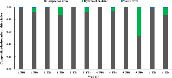 Figure 10
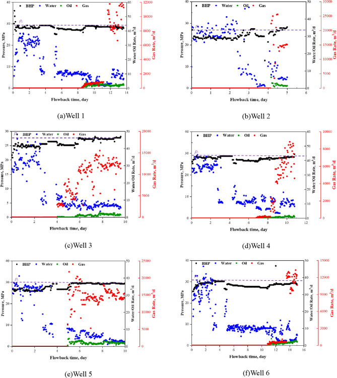 Figure 11
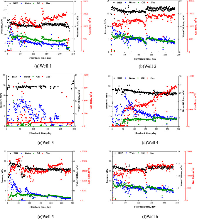 Figure 12
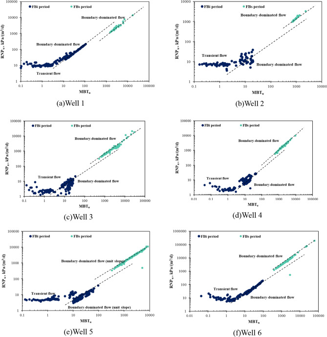 Figure 13
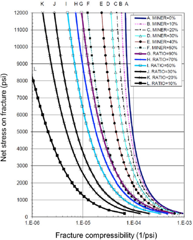 Figure 14
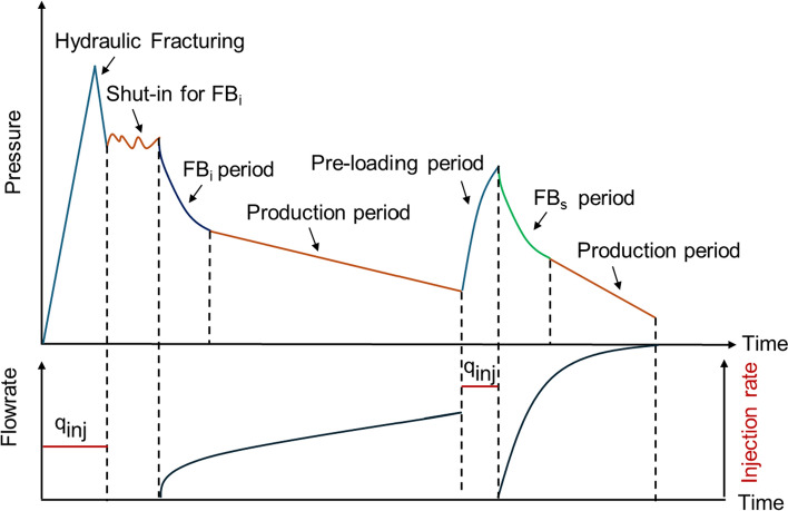 Figure 1
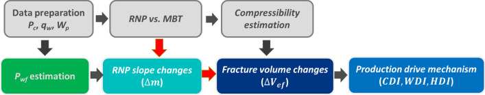 Figure 2
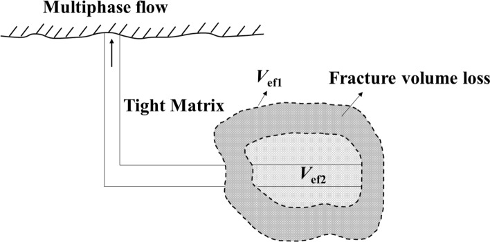 Figure 3
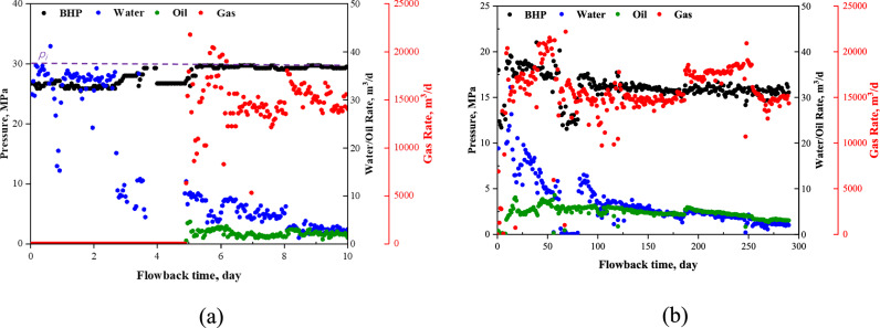 Figure 4
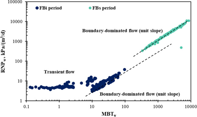 Figure 5
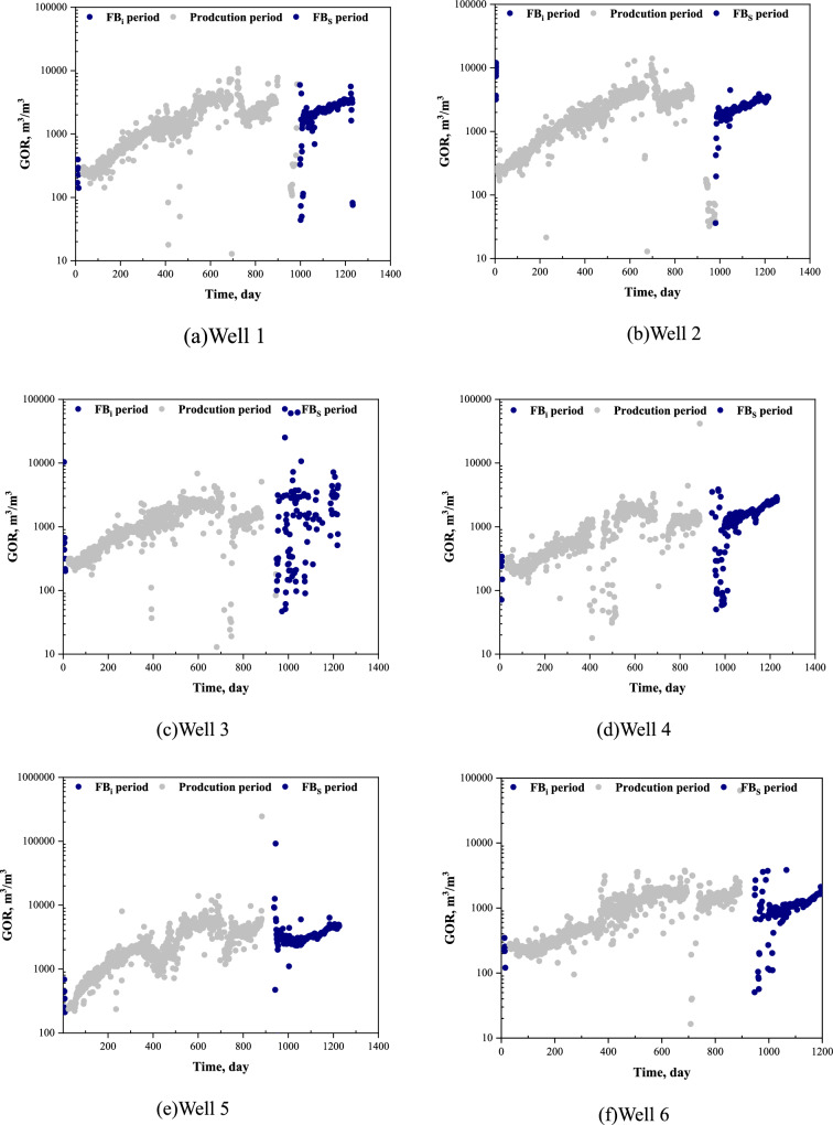 Figure 6
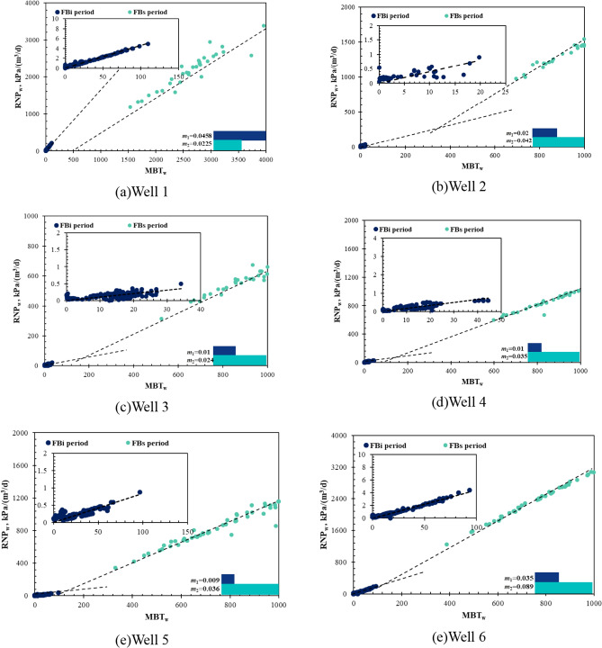 Figure 7
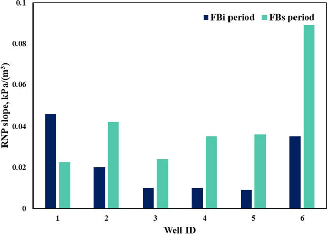 Figure 8
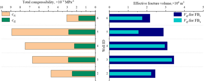 Figure 9
- —http://dx.doi.org/10.13039/501100000038Natural Sciences and Engineering Research Council of Canada
Peer Reviews
No public reviews on file for this paper yet. If you reviewed it on a platform where reviews are public (OpenReview, ICLR, NeurIPS, ICML), you can paste yours below so the community can read it here.
Videos
No videos yet. Explain this paper in a talk, walkthrough, or lecture? Add one.
Taxonomy
TopicsHydraulic Fracturing and Reservoir Analysis · Drilling and Well Engineering · Reservoir Engineering and Simulation Methods
Introduction
During the development and production of unconventional reservoirs, the fracture pressure gradually decreases as the fluid inside the fracture is gradually extracted. The changes of fracture characteristics (i.e., permeability, length, and width) with the depletion of fracture pressure are partially considered in the previous studies (Cao et al. 2022; Liu et al. 2018; Wang and Sharma 2019). Recent studies indicate that only about 25% of fracture length and 75% of effective fracture volume contribute to production over an extended production period (Gaddipati et al. 2020; Swami et al. 2017). The fracture length and permeability have been estimated by the production history matching (Jia et al. 2022; Lamidi Benson and Clarkson 2023). However, effective and robust methods for measuring fracture volume loss using flowback and production data are rarely reported.
Recently, flowback analysis has become a common practice for fracture characterization and well-performance evaluation. However, most studies have focused on characterizing the relationship between fracture permeability and pressure variation with the pressure depletion. The rate- and pressure-transient behaviors during flowback and post-flowback periods have been studied to understand the physics of flowback and to evaluate the fracture characteristics (Abbasi et al. 2014; Hossain et al. 2020, 2019; Ibrahim et al. 2019; Yang and Wu 2017). Flowback and early-time production analysis are increasingly used for fracture dynamics assessment, especially in shale gas development (Ibrahim et al. 2020; Zhang et al. 2023). Some pressure/rate transient models have been developed to investigate the effects of fracture half-length and fracture permeability on rate transient behavior (Clarkson and Williams-Kovacs 2013; Ezulike and Dehghanpour 2014; Gringarten 2008; Jia 2017; Li et al. 2019; Williams-Kovacs 2017; Zhang and Emami-Meybodi 2020a, 2020b). Moreover, several semi-analytical pressure-transient models have been applied for fracture volume estimation. The single- and multi-phase models for fracture volume estimation with pressure-supercharge effect have been proposed by Ezulike et al. 2016. Hossain et al. 2020 extended this tank model to analyze the effective stimulated reservoir volume using the post-flowback data. Moussa et al. 2020 estimated fracture volume with the changes of fracture porosity using the flowback data. Although many scholars have analyzed the changes of fracture permeability and geometry during the production processes, there remains a lack of quantitative multiphase flowback models to analyze the fracture volume loss caused by pressure depletion during production processes. Three phases (oil, gas, and water) may flow through the induced fractures, especially when the bottomhole pressure is lower than the bubble point pressure during flowback process. Therefore, three-phase flowback models are needed to be developed to capture the changes in fracture volume after long-term production processes.
Fracture closure, gas expansion, and water depletion have been considered as drive mechanisms for the flowback process. The results of Alkouh et al. 2014 show that the contribution of gas-drive mechanism (Sg_c_g) is at least 97% when the water saturation is less than 70. Fracture compressibility is generally one to two orders of magnitude higher than matrix compressibility (Newman 1973; Sawabini et al. 1974). Consequently, fracture closure serves as a key drive mechanism during FB_i_ and FB_s_ periods. In this paper, we analyze various flowback-drive mechanisms to investigate the changes in fluid-flow mechanisms between FB_i_ and FB_s_ periods.
Although infill drilling has improved the production and economic return, these practices have led to growing concern over the side effect often referred to as fracture hits between parent and infill wells. The fracture hits can cause decreased production in a parent well, as well as other negative effects such as wellbore sanding and reduced production performance in the infill well (Ajisafe et al. 2021; Jacobs 2017; King et al. 2017; Whitfield et al. 2018). The preloading strategy has been proved to be an effective and successful way to mitigate the loss of production caused by fracture hit (Aniemena et al. 2022; Joslin et al. 2020; Whitfield et al. 2018). To limit the influence of parent–child fracture hit, water is usually injected into the parent wells before the stimulation of child wells. The preloading fluid is produced back to the surface (Whitfield et al. 2018; Zheng et al. 2021). This process is referred to as the second flowback (FB_s_). It provides sufficient hourly flowback data and daily production data to quantitatively assess the changes in fracture volume from the FB_i_ period to the FB_s_ period.
The objective of this paper is to capture the changes in effective fracture volume during the production periods between the two flowback processes and compare the rate and pressure transient responses of the second flowback period with those of the initial flowback period to evaluate the changes in fracture characteristics. First, the generalized multiphase (oil, gas, and water) flowback model for FB_s_ period is proposed to evaluate the fracture volume loss between the FB_i_ period and the FB_s_ periods. Then, the fracture volume loss is estimated from the changes in the slope of RNP diagnostic plots and the variations of total compressibilities between FBi and FBs periods. Next, the RNP diagnostic plots of six multi-fractured horizontal wells completed in Niobrara and Codell formations in DJ Basin in the United States are constructed and the changes in fracture volume are compared. Finally, the compaction-drive index (CDI), hydrocarbon-drive index (HDI), and water-drive index (WDI) are used to compare the variations of production drive mechanisms during the two flowback periods.
Workflow for fracture volume loss
Timeline of initial and second flowback periods
Figure 1 illustrates the profiles of flow rate and pressure versus time from hydraulic fracturing treatment to the second flowback and subsequent production period. For the fractured horizontal wells in tight or shale reservoirs, the well is typically shut in for a period of time after hydraulic fracturing. This procedure allows more fracturing fluid to enter deeper into the reservoir and displace more oil. After the shut-in period, the well is then opened for the initial flowback (FB_i_), followed by the transition to later production. The fractures are generally filled with fracturing fluid at the beginning of the FB_i_ period. To mitigate pressure interference resulting from infill drilling, a large amount of water is injected into the parent well during the pre-loading period (Aniemena et al. 2022; Whitfield et al. 2018). In this work, the period during which the pre-loading fluid from the parent wells is produced back to the surface after the stimulation of child wells is referred to as the second flowback (FB_s_). The data from FB_i_ and FB_s_ periods are adopted in this paper to capture the loss of fracture volume due to pressure depletion during long-term production period.Fig. 1. Schematic illustration of flow rate and pressure versus time profiles
Fracture volume loss estimation
In this paper, we construct the rate-normalized pressure (RNP) diagnostic plots for both FB_i_ and FB_s_ periods. The average effective fracture volume can be estimated by the changes in RNP slope and total compressibility between FB_i_ and FB_s_ periods. The variations in effective fracture volume and production-drive mechanisms are compared for both FB_i_ and FB_s_ periods. The workflow for the estimation of fracture volume changes is shown in Fig. 2.Fig. 2. The workflow for the estimation of fracture volume changes
- Flowback data preparations: We collect initial and second flowback data, including tubing and casing pressures, along with flow rate (qw) and cumulative water production (Wp) of the parent wells. The hourly data from the initial flowback (FB_i_) and daily data from the second flowback (FB_s_) are then analyzed after noise removal.
- Pressure estimations: The bottomhole pressure data are estimated from casing pressure by using the correlation of Hagedorn and Brown 1965. The initial average reservoir pressure is estimated by averaging the flattening value of the calculated downhole pressure before hydrocarbon breakthrough as proposed by Jones et al. 2014.
- RNP diagnostic analysis: We construct the diagnostic plots of the RNP versus material-balance time (MBT) for both FB_i_ and FB_s_ data of the studied wells. RNP and MBT during FB_i_ and FB_s_ periods can be described as (Hossain et al. 2019)
Here, the subscripts FB_i_ and FB_s_ represent the initial and second flowback periods, respectively. 4. Average effective fracture volume estimation: The RNP slope (m) for both FB_i_ and FB_s_ periods can be determined from the RNP versus MBT diagnostic plots. The detailed derivation of the slope of the rate-normalized pressure (RNP) curve is provided in the model section, and it is expressed as
\documentclass[12pt]{minimal} \usepackage{amsmath} \usepackage{wasysym} \usepackage{amsfonts} \usepackage{amssymb} \usepackage{amsbsy} \usepackage{mathrsfs} \usepackage{upgreek} \setlength{\oddsidemargin}{-69pt} \begin{document}$$m({\text{slope}}) = \frac{1}{{V_{\text{ef}} c_{\text{t}} }}$$\end{document}Based on Eq. 3, the average effective fracture volume (Vef) is determined by utilizing the RNP slope and the total compressibility(Fu et al. 2017). The total compressibility is a function of the fracture, water and oil compressibility and water saturation. We assume that the water compressibility does not change between the FB_i_ and FB_s_ periods. cw is obtained from the existing correlations (Meehan 1980), and co is obtained from the pressure-dependent compressibility curves for the Niobrara Formation (Ning et al. 2018). The water saturation (Swi) of the FB_i_ period is assumed 1 since there is a long period of single-phase water production at the beginning of the FB_i_ period. Sw of the FB_s_ period can be estimated by (Ezulike and Dehghanpour 2014)
\documentclass[12pt]{minimal} \usepackage{amsmath} \usepackage{wasysym} \usepackage{amsfonts} \usepackage{amssymb} \usepackage{amsbsy} \usepackage{mathrsfs} \usepackage{upgreek} \setlength{\oddsidemargin}{-69pt} \begin{document}$$S_{\text{w}} = S_{\text{wi}} - \frac{{Q_{\text{w}} }}{{V_{\text{ef}1} }}$$\end{document}Here, Qw is the water production volume from the FB_i_ period to the start of FBs period.The primary challenge in estimating Vef lies in accurately calculating the fracture compressibility. Here, we adopt the graphical method proposed by Aguilera 1999 to estimate cpe, as shown in Appendix C. cpe is estimated using net pressure and mineralization values. The net pressure (pn) can be calculated by (Sherman and Holditch 1991)
\documentclass[12pt]{minimal} \usepackage{amsmath} \usepackage{wasysym} \usepackage{amsfonts} \usepackage{amssymb} \usepackage{amsbsy} \usepackage{mathrsfs} \usepackage{upgreek} \setlength{\oddsidemargin}{-69pt} \begin{document}$$p_{\text{n}} = p_{\text{closure}} - p_{\text{wf}}$$\end{document}Here, pclosure is the fracture closure pressure that can be approximated by the minimum horizontal principal stress. The maximum pressure during the shut-in period is used to approximate the fracture closure pressure in the absence of diagnostic pressure injection test (DFIT) (Wang et al. 2019). Therefore, the average effective fracture volume is estimated using the RNP slope, m, water saturation, Sw, average fracture compressibility,* c*pe, water compressibility, cw, and oil compressibility, co. 5. Comparing flowback drive mechanisms: Based on the definitions of total compressibility, the drive mechanisms of fracture closure, hydrocarbon expansion and water depletion can be evaluated quantitatively. The drive mechanisms for the two flowback periods are compared by calculating three flowback-drive indices (compaction-drive index (CDI), hydrocarbon-drive index (HDI), and water-drive index (WDI)) introduced by Ezulike et al. 2016:
\documentclass[12pt]{minimal} \usepackage{amsmath} \usepackage{wasysym} \usepackage{amsfonts} \usepackage{amssymb} \usepackage{amsbsy} \usepackage{mathrsfs} \usepackage{upgreek} \setlength{\oddsidemargin}{-69pt} \begin{document}$$\text{CDI} = \frac{{c_{\text{pe}} }}{{c_{\text{t}} }}$$\end{document} \documentclass[12pt]{minimal} \usepackage{amsmath} \usepackage{wasysym} \usepackage{amsfonts} \usepackage{amssymb} \usepackage{amsbsy} \usepackage{mathrsfs} \usepackage{upgreek} \setlength{\oddsidemargin}{-69pt} \begin{document}$$\text{HDI} = \frac{{S_{\text{o}} c_{\text{o}} + S_{\text{g}} c_{\text{g}} }}{{c_{\text{t}} }}$$\end{document} \documentclass[12pt]{minimal} \usepackage{amsmath} \usepackage{wasysym} \usepackage{amsfonts} \usepackage{amssymb} \usepackage{amsbsy} \usepackage{mathrsfs} \usepackage{upgreek} \setlength{\oddsidemargin}{-69pt} \begin{document}$$\text{WDI} = \frac{{S_{\text{w}} c_{\text{w}} }}{{c_{\text{t}} }}$$\end{document}Here, the sum of HDI and WDI represents fluid expansion, which can be expressed as EDI = HDI + WDI. 6. Effective fracture volume and total compressibility changes: The loss percentage of effective fracture volume (RVef) and total compressibility (Rct) during the two flowback periods can be estimated by
\documentclass[12pt]{minimal} \usepackage{amsmath} \usepackage{wasysym} \usepackage{amsfonts} \usepackage{amssymb} \usepackage{amsbsy} \usepackage{mathrsfs} \usepackage{upgreek} \setlength{\oddsidemargin}{-69pt} \begin{document}$$R_{{V_{\text{ef}} }} = \frac{{V_{\text{ef}1} - V_{\text{ef}2} }}{{V_{\text{ef}1} }}$$\end{document} \documentclass[12pt]{minimal} \usepackage{amsmath} \usepackage{wasysym} \usepackage{amsfonts} \usepackage{amssymb} \usepackage{amsbsy} \usepackage{mathrsfs} \usepackage{upgreek} \setlength{\oddsidemargin}{-69pt} \begin{document}$$R_{{c_{\text{t}} }} = \frac{{c_{\text{t}1} - c_{\text{t}2} }}{{c_{\text{t}1} }}$$\end{document}Here, Vef1 and Vef2 are the effective fracture pore volume estimated by analyzing the initial and second flowback data, respectively. ct1 and ct2 are the total compressibility estimated by analyzing the initial and second flowback data, respectively.
Methodology
Conceptual model
At the beginning of the FB_i_ period, the fractures are almost filled with fracturing water, and the fracture volume is denoted as Vef1. After a period of production, the pressure in the fractures gradually decreases. The fracture volume gradually shrinks from Vef1 to Vef2 between FBi and FBs period, as shown in Fig. 3. The FB_i_ data from the single-phase water production can be used to estimate the initial fracture volume. During the FBs stage, fluids (oil, gas and water) are gradually extracted, resulting in multiphase flow (oil, gas and water) within the fractures. Three-phase (oil, gas and water) flow occurs in the fractures especially when the bottomhole pressure drops below the bubble point pressure. The fracture volume after a long production period can be estimated from the FB_s_ data. Therefore, the fracture volume loss can be determined by comparing the fracture volume changes between FB_i_ and FB_s_ periods.Fig. 3. Schematic illustration of fracture volume loss between FBi and FBs periods
This paper hypothesizes that the changes in effective fracture volume can be evaluated by analyzing and comparing the initial and second flowback. Here, we assume that 1) the fractures are initially filled with water during FB_i_ period; 2) the fractures are filled with multiphase fluids (water + oil/gas) after injecting the preload fluids into the parent wells, and these multiphase fluids are primarily produced from the fractures during FB_s_ period; and 3) the gas expulsion from the oil is negligible under downhole conditions during the FB_i_ period. First, we test the hypothesis by analyzing the pressure and rate profiles measured during the two periods for six fractured horizontal wells. Then, we construct and compare RNP diagnostic plots for the initial and second flowback periods. Finally, we evaluate the changes in effective fracture volume by analyzing the variations in total compressibility and the slope of RNP versus MBT plots.
Multiphase flowing material balance model for FBs period
The gas expulsion from the oil under downhole conditions is considered for the second flowback period in this work. Therefore, a multiphase (oil, gas, and water) flowback model is developed in this paper. The water-phase mass conservation equations for both FB_i_ and FB_s_ in the fractures are described as (Hossain et al. 2020, 2019)
\documentclass[12pt]{minimal} \usepackage{amsmath} \usepackage{wasysym} \usepackage{amsfonts} \usepackage{amssymb} \usepackage{amsbsy} \usepackage{mathrsfs} \usepackage{upgreek} \setlength{\oddsidemargin}{-69pt} \begin{document}$$q_{{\text{w}_{{\text{in }}} }} \rho_{\text{w}} - q_{{\text{w}_{{\text{out }}} }} \rho_{\text{w}} = \frac{\partial }{\partial t}\left( {\rho_{\text{w}} V_{\text{w}} } \right)$$\end{document}Since the water influx from the matrix is negligible as assumed in the previous section, Eq. (11) can be rewritten as
\documentclass[12pt]{minimal} \usepackage{amsmath} \usepackage{wasysym} \usepackage{amsfonts} \usepackage{amssymb} \usepackage{amsbsy} \usepackage{mathrsfs} \usepackage{upgreek} \setlength{\oddsidemargin}{-69pt} \begin{document}$$0 - q_{\text{w}} \rho_{\text{w}} = \frac{\partial }{\partial t}\left( {\rho_{\text{w}} V_{\text{w}} } \right)$$\end{document}The water volume in the effective fracture volume is given by
\documentclass[12pt]{minimal} \usepackage{amsmath} \usepackage{wasysym} \usepackage{amsfonts} \usepackage{amssymb} \usepackage{amsbsy} \usepackage{mathrsfs} \usepackage{upgreek} \setlength{\oddsidemargin}{-69pt} \begin{document}$$V_{\text{w}} = V_{\text{ef}} - V_{\text{o}} - V_{\text{g}}$$\end{document}Equation (12) is rewritten using the definition of Vw as
\documentclass[12pt]{minimal} \usepackage{amsmath} \usepackage{wasysym} \usepackage{amsfonts} \usepackage{amssymb} \usepackage{amsbsy} \usepackage{mathrsfs} \usepackage{upgreek} \setlength{\oddsidemargin}{-69pt} \begin{document}$$- q_{\text{w}} \rho_{\text{w}} = V_{\text{w}} \frac{{\partial \rho_{\text{w}} }}{\partial t} + \rho_{\text{w}} \left( {\frac{{\partial V_{\text{ef}} }}{\partial t} - \frac{{\partial V_{\text{o}} }}{\partial t} - \frac{{\partial V_{\text{g}} }}{\partial t}} \right)$$\end{document}Equation (14) can be further expanded using the chain rule as
\documentclass[12pt]{minimal} \usepackage{amsmath} \usepackage{wasysym} \usepackage{amsfonts} \usepackage{amssymb} \usepackage{amsbsy} \usepackage{mathrsfs} \usepackage{upgreek} \setlength{\oddsidemargin}{-69pt} \begin{document}$$- q_{\text{w}} \rho_{\text{w}} = V_{\text{w}} \frac{{\partial \rho_{\text{w}} }}{\partial P} \times \frac{\partial P}{{\partial t}} + \rho_{\text{w}} \left( {\frac{{\partial V_{\text{ef}} }}{\partial P} \times \frac{\partial P}{{\partial t}} - \frac{{\partial V_{\text{o}} }}{\partial P} \times \frac{\partial P}{{\partial t}} - \frac{{\partial V_{\text{g}} }}{\partial P} \times \frac{\partial P}{{\partial t}}} \right)$$\end{document}Here, oil and gas compressibility, defined as the changes in volume with respect to pressure, is simplified as the volume variation with pressure. The oil and gas compressibility can be defined as
\documentclass[12pt]{minimal} \usepackage{amsmath} \usepackage{wasysym} \usepackage{amsfonts} \usepackage{amssymb} \usepackage{amsbsy} \usepackage{mathrsfs} \usepackage{upgreek} \setlength{\oddsidemargin}{-69pt} \begin{document}$$c_{\text{g}} = - \frac{1}{{V_{\text{g}} }}\frac{{\partial V_{\text{g}} }}{\partial P}$$\end{document} \documentclass[12pt]{minimal} \usepackage{amsmath} \usepackage{wasysym} \usepackage{amsfonts} \usepackage{amssymb} \usepackage{amsbsy} \usepackage{mathrsfs} \usepackage{upgreek} \setlength{\oddsidemargin}{-69pt} \begin{document}$$c_{\text{o}} = - \frac{1}{{V_{\text{o}} }}\frac{{\partial V_{\text{o}} }}{\partial P}$$\end{document}Based on the definition of fracture, water, oil, and gas compressibility in Appendix A, Eq. (15) can be written as
\documentclass[12pt]{minimal} \usepackage{amsmath} \usepackage{wasysym} \usepackage{amsfonts} \usepackage{amssymb} \usepackage{amsbsy} \usepackage{mathrsfs} \usepackage{upgreek} \setlength{\oddsidemargin}{-69pt} \begin{document}$$- q_{\text{w}} = V_{\text{w}} c_{\text{w}} \frac{\partial P}{{\partial t}} + \left( {V_{\text{ef}} c_{\text{f}} + V_{\text{o}} c_{\text{o}} + V_{\text{g}} c_{\text{g}} } \right)\frac{\partial P}{{\partial t}}$$\end{document}The equation is further expanded as
\documentclass[12pt]{minimal} \usepackage{amsmath} \usepackage{wasysym} \usepackage{amsfonts} \usepackage{amssymb} \usepackage{amsbsy} \usepackage{mathrsfs} \usepackage{upgreek} \setlength{\oddsidemargin}{-69pt} \begin{document}$$- q_{\text{w}} = V_{\text{ef}} \left[ {c_{\text{f}} + S_{\text{w}} c_{\text{w}} + S_{\text{o}} c_{\text{o}} + S_{\text{g}} c_{\text{g}} } \right]\frac{\partial P}{{\partial t}}$$\end{document}Based on the definition of total compressibility, Eq. (19) can be written as
\documentclass[12pt]{minimal} \usepackage{amsmath} \usepackage{wasysym} \usepackage{amsfonts} \usepackage{amssymb} \usepackage{amsbsy} \usepackage{mathrsfs} \usepackage{upgreek} \setlength{\oddsidemargin}{-69pt} \begin{document}$$- q_{\text{w}} = V_{\text{ef}} c_{\text{t}} \frac{\partial P}{{\partial t}}$$\end{document}Integrating both sides of Eq. (20), we have
\documentclass[12pt]{minimal} \usepackage{amsmath} \usepackage{wasysym} \usepackage{amsfonts} \usepackage{amssymb} \usepackage{amsbsy} \usepackage{mathrsfs} \usepackage{upgreek} \setlength{\oddsidemargin}{-69pt} \begin{document}$$\text{RNP}_{\text{w}} = \frac{1}{{V_{\text{ef}} c_{\text{t}} }}\text{MBT}_{\text{w}}$$\end{document}The corresponding mathematical models and detailed derivations are provided in Appendix A. From Eq. (21), the changes in RNP slope represent the combined changes in both Vef and ct.
Here, RNP_w_ is the difference between the initial reservoir pressure (pi) and the flowing bottomhole pressure (pwf) divided by the water rate (qw). MBT_w_ denotes the sum of cumulative water production (Wp) divided by the water rates. RNP_w_ and MBT_w_ are respectively given by
\documentclass[12pt]{minimal} \usepackage{amsmath} \usepackage{wasysym} \usepackage{amsfonts} \usepackage{amssymb} \usepackage{amsbsy} \usepackage{mathrsfs} \usepackage{upgreek} \setlength{\oddsidemargin}{-69pt} \begin{document}$$\text{RNP}_{\text{w}} = \frac{{p_{\text{i}} - p_{\text{wf}} }}{{q_{\text{w}} }}$$\end{document} \documentclass[12pt]{minimal} \usepackage{amsmath} \usepackage{wasysym} \usepackage{amsfonts} \usepackage{amssymb} \usepackage{amsbsy} \usepackage{mathrsfs} \usepackage{upgreek} \setlength{\oddsidemargin}{-69pt} \begin{document}$$\text{MBT}_{\text{w}} = \frac{{W_{\text{p}} }}{{q_{\text{w}} }}$$\end{document}Equation (21) describe a linear relationship between RNP_w_ and MBT_w_, characterized by a unit slope on a log/log diagnostic plot. Once ct is determined, the effective fracture volume (Vef) can be obtained from the RNP slope in the Cartesian coordinate. Therefore, Vef in both FB_i_ and FB_s_ periods can be analyzed and compared.
If the flowing bottomhole pressure is higher than the bubble point pressure, the gas expulsion from the oil under downhole conditions is negligible. It indicates two-phase (oil and water) flow under the downhole conditions. Therefore, the multiphase flow model can be simplified as a two-phase flow and Eq. (19) can be simplified as
\documentclass[12pt]{minimal} \usepackage{amsmath} \usepackage{wasysym} \usepackage{amsfonts} \usepackage{amssymb} \usepackage{amsbsy} \usepackage{mathrsfs} \usepackage{upgreek} \setlength{\oddsidemargin}{-69pt} \begin{document}$$- q_{\text{w}} = V_{\text{ef}} \left[ {c_{\text{f}} + S_{\text{w}} c_{\text{w}} + S_{\text{o}} c_{\text{o}} } \right]\frac{\partial P}{{\partial t}}$$\end{document}As shown in Eq. (24), the most significant distinction between the two-phase model and the three-phase model is the absence of the gas term in the total compressibility.
Model Application
Reservoir and well completion information
To test the hypothesis presented in the methodology section, we analyze FB_i_ and FBs data from six parent wells completed in Niobrara and Codell formations in DJ Basin. The reservoir and well-completion data for these six wells are listed in Table 1. It includes total vertical depth (TVD), number of stages (ns), gross perforated interval (GPI), total injected proppant mass (Mprop), total injected water volume (TIV), the shut-in period for initial flowback (tsh), the duration of production period (tp). TVD of the six wells varies from 2126 to 2202 m. These wells were fractured in 52–70 stages. Mprop is 4.69 to 4.76 × 10^6^ kg. Figure 1 schematically illustrates the operational events occurring during the life of these wells. tsh represents the period from the completion date to the start date of initial flowback, ranging from 5 to 37 days. Compared to the other five wells, well 1 has the shortest tsh of 5 days. tp represents the interval from the end date of FB_i_ period to the start date of shut-in period before the FB_s_ period, ranging from 860 to 890 days.Table 1. Reservoir and well-completion dataWell IDTVD (m)n_s_GPI (m)TIV (m^3^)Mprop (10^6^ kg)tsh (d)tp (d)Well 1217169315826,4284.695885Well 2215969315826,2844.6922869Well 3220252314226,8074.7237869Well 4216370316726,3324.7626874Well 5212669313925,8834.6930870Well 6213770316726,0094.7620875
Bottomhole pressure and rate profiles
Figure 4a and b show the hourly measured FB_i_ data and the daily measured FB_s_ data of well 5 (the estimated bottom pressure, and flowrates of water, oil, and gas), respectively. The dashed line represents the estimated initial average reservoir pressure. There is a long period of single-phase water production before the oil and gas breakthrough during the FB_i_ period. The average bottomhole pressure in the FB_i_ period is about 20–30 MPa, while in the FB_s_ period it is about 10–20 MPa. The bottomhole pressure and rate profiles for the other five wells during FB_i_ and FB_s_ periods are shown in Appendix B.Fig. 4. Bottomhole pressure and rate profiles of Well 5 during FB_i_ and FB_s_ periods. a Hourly measured initial flowback data; b Daily measured second flowback data. The duration of production period between the two flowback periods is 870 days
For the FB_i_ period, the long period of single-phase water production before the oil and gas breakthrough indicates that the fracture system is almost completely filled with fracturing water during the FB_i_ period. Second, the straight line with unit slope is observed in Fig. 5, suggesting the single-phase water is mainly from the fractures during the FB_i_. In other words, the water influx from the matrix into the fractures can be assumed to be negligible. During the FB_s_ period, the water is produced with hydrocarbon indicating that the fractures have multiphase fluids. The straight line with unit slope is also observed in the FB_s_ periods, indicating the water influx from matrix is negligible during FB_s_.Fig. 5. Preliminary analysis of the initial and secondary flowback periods
As shown in Figs. 6a–d and Fig. 6f, there is no significant increase in gas-oil ratio (GOR) for Well 1 ~ Well 4 and Well 6 from the start of FB_i_ period to the end of FB_s_ period. Although the bottomhole pressure decreases during the second flowback period, the insignificant changes in the GOR curve indicates that the bottomhole pressure is still higher than the bubble point pressure. In other words, the gas expulsion from the oil can be negligible under downhole conditions and the changes in fracture volume of these five wells can be analyzed using the simplified two-phase model. In contrast, Fig. 6e shows a significant increase (by more than an order of magnitude) in the GOR curve during the FBs period for Well 5, suggesting the presence of 3-phase flow (oil, gas and water) under the downhole conditions. Therefore, the multiphase flow model proposed in this paper needs to be adopted to accurately capture the changes in the fracture volume for well 5.Fig. 6GOR profiles of six wells from FB_i_ to FB_s_ flowback periods
Results and discussions
Analyzing the FBi and FBs data
Figure 7 shows the RNP versus MBT diagnostic plots for the initial and second flowback periods of the studied parent wells. In order to quantitatively compare the flowback responses of the two periods, the RNP slopes for FB_i_ (m1) and for FB_s_ (m2) are compared in Fig. 8. In general, the RNP slope increases by approximately 2–5 times during the second flowback compared to the initial flowback, except for well 1. Interestingly, a straight line with unit slope is also observed in the RNP plot of the FB_s_ period where water is produced with hydrocarbons. This suggests negligible water influx from matrix and indicates that oil expansion serves as a drive mechanism for the pseudo-steady state flow of water, as described by Eq. (18). This also suggests that the fracture hit might have been avoided, as the closed-tank system of water is not interrupted by completing the child wells. Therefore, the increase in RNP slope with pressure depletion (5–10 MPa) from FB_i_ to FB_s_ period might be caused by the loss of effective fracture volume and the reduction in total compressibility due to partial fracture closure. The observed decrease in the RNP slope of well 1 may be attributed to an increase in total compressibility or the lower initial Vef compared to the other wells, as discussed later.Fig. 7RNP vs MBT diagnostic plots of the six wells during the FBi and FBs periodsFig. 8Comparing the RNP slope of the six wells during initial and second flowback periods
Effective fracture volume estimation
Figure 9 shows the calculated Vef, \documentclass[12pt]{minimal} \usepackage{amsmath} \usepackage{wasysym} \usepackage{amsfonts} \usepackage{amssymb} \usepackage{amsbsy} \usepackage{mathrsfs} \usepackage{upgreek} \setlength{\oddsidemargin}{-69pt} \begin{document}$${R}_{{V}_{\text{ef}}}$$\end{document} , \documentclass[12pt]{minimal} \usepackage{amsmath} \usepackage{wasysym} \usepackage{amsfonts} \usepackage{amssymb} \usepackage{amsbsy} \usepackage{mathrsfs} \usepackage{upgreek} \setlength{\oddsidemargin}{-69pt} \begin{document}$${R}_{{c}_{\text{t}}}$$\end{document} by analyzing the flowback data from the two flowback periods. \documentclass[12pt]{minimal} \usepackage{amsmath} \usepackage{wasysym} \usepackage{amsfonts} \usepackage{amssymb} \usepackage{amsbsy} \usepackage{mathrsfs} \usepackage{upgreek} \setlength{\oddsidemargin}{-69pt} \begin{document}$${R}_{{V}_{\text{ef}}}$$\end{document} and \documentclass[12pt]{minimal} \usepackage{amsmath} \usepackage{wasysym} \usepackage{amsfonts} \usepackage{amssymb} \usepackage{amsbsy} \usepackage{mathrsfs} \usepackage{upgreek} \setlength{\oddsidemargin}{-69pt} \begin{document}$${R}_{{c}_{\text{t}}}$$\end{document} are estimated using Eqs. (28) and (29). Compared to the FB_i_ period, ct and Vef for the five wells are decreased during the FB_s_ period. Although the total compressibility is decreased due to the pressure depletion from FB_i_ to FB_s_ periods, a loss of Vef is still observed, with \documentclass[12pt]{minimal} \usepackage{amsmath} \usepackage{wasysym} \usepackage{amsfonts} \usepackage{amssymb} \usepackage{amsbsy} \usepackage{mathrsfs} \usepackage{upgreek} \setlength{\oddsidemargin}{-69pt} \begin{document}$${R}_{{V}_{\text{ef}}}$$\end{document} values estimated at 3%–45%. The pressure profiles show that the bottomhole pressure is reduced by 5–10 MPa from the FB_i_ to the FB_s_ periods. Therefore, the high values of \documentclass[12pt]{minimal} \usepackage{amsmath} \usepackage{wasysym} \usepackage{amsfonts} \usepackage{amssymb} \usepackage{amsbsy} \usepackage{mathrsfs} \usepackage{upgreek} \setlength{\oddsidemargin}{-69pt} \begin{document}$${R}_{{V}_{\text{ef}}}$$\end{document} may be attributed to fracture closure caused by pressure depletion between the two flowback periods (Wang et al. 2019). Moreover, the initial Vef of well 1 is approximately 1.4 × 10^4^ m^3^, which is lower than the average Vef for the other five wells. This may explain the relatively higher slope of RNP plot for well 1 during the FB_i_ period.Fig. 9. Estimations and variations of Vef and ct for the FB_i_ and FB_s_ periods. \documentclass[12pt]{minimal} \usepackage{amsmath} \usepackage{wasysym} \usepackage{amsfonts} \usepackage{amssymb} \usepackage{amsbsy} \usepackage{mathrsfs} \usepackage{upgreek} \setlength{\oddsidemargin}{-69pt} \begin{document}$${R}_{{c}_{\text{t}}}$$\end{document} and \documentclass[12pt]{minimal} \usepackage{amsmath} \usepackage{wasysym} \usepackage{amsfonts} \usepackage{amssymb} \usepackage{amsbsy} \usepackage{mathrsfs} \usepackage{upgreek} \setlength{\oddsidemargin}{-69pt} \begin{document}$${R}_{{V}_{\text{ef}}}$$\end{document} are defined by Eqs. (14) and (15)
Analyzing the production drive mechanisms
Based on the RNP slope, three drive indices are calculated for the initial and second flowback periods, as shown in Fig. 10. The compaction drive index (CDI), as the dominant mechanism, varies from 0.54 to 1 during the two flowback periods. However, compared to the initial flowback period, the CDI decreases by 16% on average for the five wells. In other words, the contribution of fracture closure as a driving mechanism is lower during the FB_s_ period compared with that during the FB_i_ period. The reduction in CDI is compensated by a 16% increase in EDI (EDI = HDI + WDI) during the FB_s_ period. For well 1, there is about 6% increase in HDI during the FB_s_ period. The greater hydrocarbon expansion might account for the decreased slope in the RNP versus MBT diagnostic plot during FB_s_. As a result, the overall increase in hydrocarbon compressibility for well 1 may explain the decrease in its RNP slope during the FBs period.Fig. 10. Variations of compaction-, water- and hydrocarbon-drive indices for the FB_i_ and FB_s_ periods
Comparative analysis of two-phase and multiphase flow model for Well 5
To illustrate the difference in fracture volume analysis of FB_s_ between the multiphase model and the simplified two-phase model considering the significant increase in GOR curve (by more than an order of magnitude), both models are applied to analyze the loss of fracture volume for well 5, as shown in Table 2.Table 2. Comparative analysis of two-phase and multiphase flow model for Well 5ParametersSimplified two-phase modelThree-phase modelS_w_0.6350.635S_o_0.3650.022Sg/0.343c_t_1.66 × 10^–4^2.86 × 10^–4^Vef (m^3)^26,60315,440CDI0.920.54HDI0.060.46WDI0.010.01
As shown in Table 2, there is a significant deviation in the estimated fracture volume during the FBs period, which can be attributed to changes in total compressibility. In essence, the total compressibility depends on the variations in oil and gas saturation. Regarding the drive index, the increase in HDI compensates for the decrease in CDI. It is the result of the significant gas expulsion under downhole conditions. Therefore, the three-phase model is recommended for analyzing fracture volume loss from FBi to FBs periods in the parent wells where the GOR increases significantly.
Limitations and future work
This paper provides a workflow for evaluating the changes in fracture characteristics between initial and second flowback of parent wells. For the estimation of the effective fracture volume using the slope of RNP plots, the assumptions related to compressibility evaluation bring some uncertainties: (1) The initial free gas in fractures during FB_s_ is uncertain since the bubble-point pressure is not provided. (2) The fracture compressibility is obtained from the graphical method, where the approximation of fracture closure pressure and mineralization ratio both bring some uncertainties to the estimated fracture compressibilities. (3) The oil in fractures during the initial flowback period is neglected in this work, and the initial water saturation during the second flowback period is uncertain, both contributing to uncertainties in total compressibility. The relatively low number of parent wells makes it challenging to obtain accurate correlations between completion-design parameters and fracture volume loss. However, this work is a step forward in analyzing flowback data at different stages and comparing fracture characteristics. Future studies can focus on collecting a larger number of parent wells with reservoir, completion, and production data to estimate fracture compressibility and develop correlations between completion parameters and fracture volume loss.
Summary and conclusions
The first and second flowback data from six parent wells were analyzed and compared to evaluate the changes in effective fracture volume during the production period. The RNP diagnostic plots of the six parent wells, completed in Niobrara and Codell formation, were constructed for both FBi and FBs periods to estimate the changes in effective fracture volume. Based on the analysis, the following conclusions were drawn:
- The comparative analysis of the initial and second flowback data can be used to estimate the changes in effective fracture volume. This paper presents a flowback model and workflow for estimating fracture volume changes, which includes flowback data preparations, bottomhole pressure estimations, RNP diagnostic analysis, average fracture volume estimation and comparison of flowback drive mechanisms.
- The RNP versus MBT diagnostic plots generally show an around 2–5 times increase in the slope during the second flowback period. The increase in RNP slope with pressure depletion (5–10MPa) from FB_i_ to FB_s_ period might be attributed to the loss of effective fracture volume and the reduction in total compressibility due to partial fracture closure.
- The effective fracture volume during the two flowback periods can be quantitatively estimated using the RNP slope and total compressibility. The percentage of effective fracture volume loss between the initial and second flowback periods is estimated at 3%–45%.
- Compaction drive is identified as the dominant mechanism during both periods. The calculations show a 16% decrease in the compaction drive index during the second flowback period compared to the initial period. The reduction in the compaction-drive index is compensated by an increase in the hydrocarbon-drive index during the second flowback period.