Unified Framework for Molecular Response Functions of Different Electronic-Structure Models
Bin Gao, Magnus Ringholm

TL;DR
This paper introduces SymResponse, a flexible framework for calculating molecular response functions using various electronic-structure models.
Contribution
The novelty is a unified symbolic framework that simplifies implementing and extending response theory across different models.
Findings
SymResponse uses symbolic expressions to represent response functions for numerical evaluation.
The framework is demonstrated with Hartree–Fock, DFT, and coupled-cluster methods.
Elimination rules reduce computational effort in response calculations.
Abstract
A unified framework—SymResponse—has been developed as a versatile tool to aid the implementation of response theory for different electronic-structure models. The framework manipulates the quasi-energy formulation of response theory at a symbolic level by building on top of other well-developed symbolic libraries. Response functions can therefore be nicely represented by “symbolic expressions,” which can be further evaluated numerically by users by developing their own evaluation routines with the assistance of SymResponse. The design of SymResponse makes it extensible to different electronic-structure models with only a moderate further amount of development effort. Response theory at Hartree–Fock, density functional theory, and coupled-cluster levels has been implemented in the present work as a demonstration, where elimination rules [KristensenK.J. Chem. Phys.2008, 129,…
Genes, proteins, chemicals, diseases, species, mutations and cell lines named across the full text — each resolved to its canonical identifier and authoritative record.
Click any figure to enlarge with its caption.
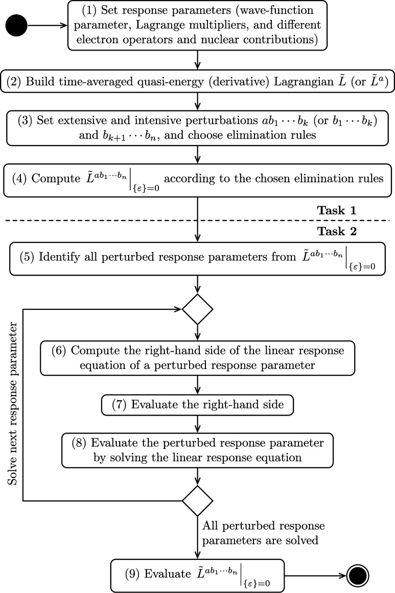 Figure 1
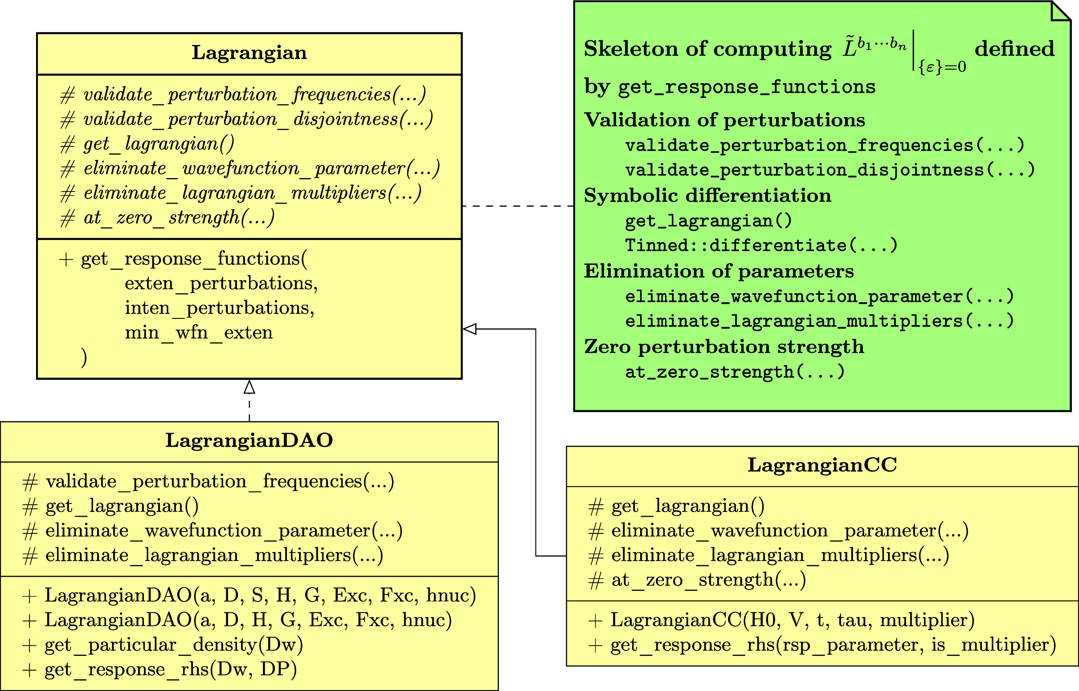 Figure 2
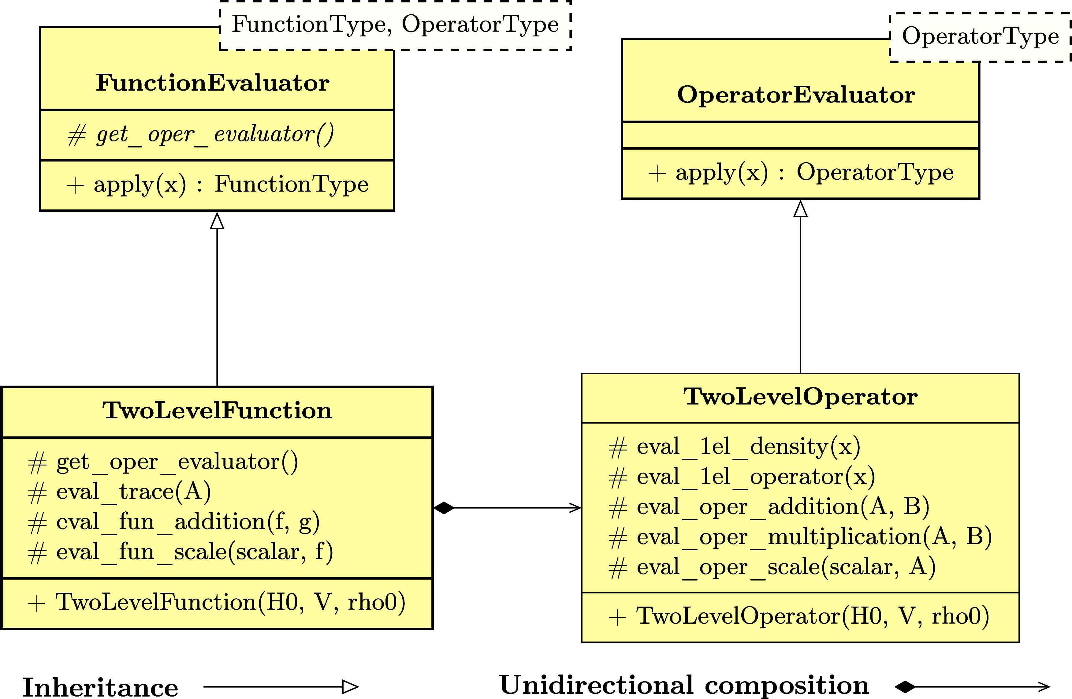 Figure 3
| classes and helper functions | description |
|---|---|
| A C++ | |
| A (response) parameter with a given name. The parameter will depend on all perturbations to arbitrary order. It can be used to represent, for example, Lagrangian multipliers. | |
| Remove the following quantities from | |
| differentiate | |
| eliminate a
given response | |
| write | |
| make a conjugate transpose of | |
| replace some symbols with others (specified by the
parameter |
- —Norges ForskningsrÃ¥d10.13039/501100005416
Peer Reviews
No public reviews on file for this paper yet. If you reviewed it on a platform where reviews are public (OpenReview, ICLR, NeurIPS, ICML), you can paste yours below so the community can read it here.
Videos
No videos yet. Explain this paper in a talk, walkthrough, or lecture? Add one.
Taxonomy
TopicsAdvanced Chemical Physics Studies · Photochemistry and Electron Transfer Studies · Spectroscopy and Quantum Chemical Studies
Introduction
1
The calculation of molecular properties has been and will stay an active research field in computational chemistry, as such calculations work as a bridge between theory and experiment. From the side of theoretical studies, the simulation of molecular properties involves solving the time-dependent Schrödinger equation under external (and usually time-dependent) influences. If these influences or perturbations are sufficiently weak, this can be carried out by perturbation-theory approaches. Such an approach in the framework of the Hartree–Fock approximation can be dated back to 1964 by Ball and McLachlan.^1,2^
After the seminal work by Runge and Gross^3^ in 1984, many efforts have been devoted to obtaining information about electronically excited states within the framework of time-dependent density functional theory (TDDFT). One important such contribution is by Casida in 1990s,^4,5^ in which the information on excited states is derived as a linear response to an applied perturbation. Over the last few decades, impressive achievements have been made in the use of response theory to calculate molecular properties. Such developments are mostly based on the pioneering work of Olsen and Jørgensen^6^ in 1985, in which they for the first time devised a general way of calculating higher-order response functions for self-consistent field (SCF) and multiconfigurational SCF (MCSCF) noneigenstates of the unperturbed molecular Hamiltonian. Later on, the quasi-energy approach was developed,^7−9^ in which frequency-dependent response functions could be conveniently derived from the derivatives of the time-averaged quasi-energy with respect to external perturbations. The so-called 2n + 1 and 2n + 2 rules could be routinely used for a properly chosen Lagrangian to judiciously eliminate the need to calculate some response parameters during calculations^8,10^ and thereby offering an opportunity to reduce the computational task size.
So far, the quasi-energy approach has been successfully applied to different electronic-structure models, for instance, Hartree–Fock (HF) and DFT, MCSCF, configuration interaction (CI) and coupled-cluster (CC) theory.^8,11,12^ Relatively recently, Thorvaldsen and co-workers proposed an atomic orbital (AO) density matrix-based quasi-energy formulation of the response theory at the HF and DFT levels.^13^ By its open-ended formulation, their approach can be employed to calculate a wide range of molecular properties with time- and perturbation-dependent basis sets and relativistic or nonrelativistic Hamiltonians.^14,15^ In a more recent work, Ringholm, Jonsson and Ruud presented a new implementation of this open-ended response theory formulation by using the technique of recursive programming.^16^ Their implementation has made it possible to manage the calculation of a large selection of response properties of molecular systems in an analytic manner, limited by the generality of modules for, e.g., differentiated one- and two-electron integral contributions to which this implementation is connected. An implementation of the recursive approach to the calculations of single residues of response functions has also been reported by Friese, Ringholm, Ruud and their co-workers.^17,18^
It is undoubtedly attractive to extend such open-ended recursive capability to other electronic-structure models, such as the MCSCF, CI and CC levels of theory, which are not supported in the aforementioned formulation.^13^ This can be considered in light of the observation that standard grids and aspects of the functionals themselves may be problematic when it comes to the integration of exchange-correlation (XC) functionals and their derivatives as in the case of higher-order polarizabilities^15,19^ and properties related to vibrational spectroscopies.^20^ Furthermore, and perhaps more simply, this can also be motivated by the desire to calculate analytically a wide variety of molecular properties at accuracies unattainable by the HF and DFT approaches.
However, algorithms and software development of the aforementioned recursive approach^16−18^ are specially designed for the AO density matrix and hardly reusable for other electronic-structure models. We therefore in this paper propose a new unified framework called SymResponse,^21^ which is a tool for the simulation of molecular response functions and is extensible to different electronic-structure models, offering significant reusability. The key to extensibility and reusability is an explicit separation between symbolic computations and actual evaluation in the quasi-energy formulation of response theory. The separation is achieved by building on earlier work by Gao^22,23^ where key operators and function(al)s are programmed to different C++ symbolic classes, so that response functions can be computed straightforwardly from symbolic arithmetic and differentiation. SymResponse is designed to generate hierarchical symbolic representations of the contributions to the terms one would need to evaluate for a desired property at a given level of theory. It will provide such a representation at a significant “depth” or level of detail, and while functionality for the actual (numerical) evaluation of the contributions identified by SymResponse must be supplied externally, SymResponse nevertheless offers the opportunity to significantly ease the development and maintenance effort in this area.
As a demonstration, we will in this work present the implementation of AO density matrix-based^13^ and coupled-cluster^8^ response theories in SymResponse. To illustrate the functionality, we will apply it to the evaluation of response functions of a two-level atom model within the AO density matrix-based response theory, where response functions can be evaluated analytically.^24^ Our results highlight the capabilities of SymResponse to automate the obtainment of response function expressions as these expressions become increasingly complicated at higher orders of perturbation.
The rest of this paper is organized as follows: First, we will briefly describe the theoretical background applied in the current work—the quasi-energy response theory in AO density matrix-based^13^ and coupled-cluster^8,11,25,26^ formulation. Next, we will present the design and implementation of SymResponse, and special consideration will be given to good code reusability when extending to include more electronic-structure models. Then, we will demonstrate the functionality of SymResponse by applying it to the computations of response functions within the AO density matrix-based and coupled-cluster response theories, in particular the two-level atom model will be investigated in the case of the AO density matrix-based formulation. Finally, we will give our concluding remarks and future work.
Theoretical Background
2
We will in this section consider basic expressions of the AO density matrix-based and coupled-cluster response theories. We here choose the quasi-energy derivative formulation and start from a phase-isolated state |Φ(t)⟩^13^
where the Hamiltonian Ĥ(t) is expressed as
where Ĥ0 is a time-independent unperturbed Hamiltonian, and V̂(t) is a time-dependent operator for some applied perturbation or perturbations. The quantity Q(t) is the time-dependent quasi-energy
and is a real-valued function when the Hamiltonian Ĥ(t) is Hermitian.^8,13^
It is Q(t) or the time-dependent quasi-energy Lagrangian^8,12^
which forms the starting point for approaches for the obtainment of molecular properties described in this work. Here e(t) represents constraints that the system has to obey, such as the time-dependent self-consistent-field (TDSCF) equation and the idempotency constraint in the AO density matrix-based response theory, or the amplitude equations in the coupled-cluster response theory. λ̅(t) contains the associated time-dependent Lagrangian multipliers.
A fundamental aspect of the quasi-energy derivative method is that we require V̂(t) to be periodic with a period T, and we express it on a general form^15^
where εA(t) is a real-valued time-periodic function representing the perturbation strength of the time-independent one-electron operator Â. To ensure the hermiticity of V̂(t), the operator  should be Hermitian.
The sum in the brackets [···] of eq 5 is the Fourier series of εA(t). In order for εA(t) to be real-valued, its Fourier series should contain both frequencies ω_A_ and −ω_A, and the complex Fourier coefficients εωA__ should satisfy ε–ωA_ = εωA__^^. Due to the assumed periodicity of V̂(t), each frequency ω_A_ can be expressed as an integer z_A_ times some fundamental frequency ω_A_ = z_A*ω_0. Still because of the periodicity of V̂(t), the Hamiltonian Ĥ and the state |Φ(t)⟩ are also time-periodic with the same period T. One can therefore consider the time-averaged quasi-energy Lagrangian
which fulfills the variational condition
The molecular response functions can be related to the time-averaged quasi-energy Lagrangian as^8,12^
where
and where {ε} = 0 denotes the evaluation at zero perturbation strength, i.e., εωA, εωB1, ···, εωBn = 0.
To evaluate the response functions in eq 8, a typical procedure is to first identify all required quantities involved in this equation, and then to compute these quantities from the equation of motion as deduced from the variational condition, eq 7.^8^
In the following subsections, we will first introduce the necessary definitions and notations about perturbations and derivatives for the current work. Next, we will describe key formulas of the response functions and response equations in the AO density matrix-based and coupled-cluster formulation, as well as the use of elimination rules to reduce the number of response parameters to be solved.^10,13,16^
Perturbations and Derivatives
2.1
We will in this section establish some concepts related to collections of perturbations that will be useful in the derivation to come. Here, a perturbation a can be associated with characteristics such as its perturbation strength εωA__, the associated operator Â, or the frequency ω_A_. Two perturbations are equivalent or the same if and only if they have the same characteristics.
Throughout the present work, we use “perturbation multichain” to represent derivatives with respect to perturbation strength. We define a perturbation multichain(27) as a totally ordered multiset of perturbations a ≤ b ≤ c ≤ ···, and is denoted as abc··· for the sake of simplicity. We note that the specific way in which the binary relation “≤” is defined is arbitrary for the purposes of this presentation.
Derivatives with respect to perturbation strength can thus be expressed in a more compact way by using the perturbation multichain notation. For example, derivatives of the time-averaged quasi-energy Lagrangian (8) can be written as . We notice that the notion of a perturbation collection/tuple or a totally ordered tuple of perturbation strengths have also been proposed and used in expressing these derivatives.^13,22,28^ Our perturbation multichain can be viewed as a “totally ordered” tuple^27^ of perturbations with respect to which derivation of response-theory expressions can be straightforwardly performed.
As with the totally ordered tuple of perturbation strengths,^22^ the following properties hold for the perturbation multichain:
- 1.The length of a perturbation multichain is the order of its corresponding derivative;
- 2.Perturbations that are equivalent according to the binary relation “≤” must always be consecutive in the multichain. For example, abbc can be a valid perturbation multichain, but abcb is not.
- 3.Multichains abc ≠ acb, because b ≤ c in the former case while c ≤ b in the latter case.These two multichains may represent derivatives stored in tensors with different shapes. For example, let a, b and c be the electric dipole, magnetic dipole and geometrical perturbations. The shapes of derivative tensors are (3, 3, 3N) and (3, 3N, 3) respectively for multichains abc and acb, where N is the number of atoms.
To represent derivatives of a product in response theory in a more practical manner, we will also use the concept “perturbation index chain” and its “set partition”. A perturbation index chain^22^ is a totally ordered set (or a chain) {1, ···, n} whose elements are unique and each points at the position of its corresponding perturbation in a perturbation multichain b1 ··· bn, or with a more short-hand notation, b{1, ···, n}. The set partition^22,29^ of a perturbation index chain {1, ···, n} is a collection of k (1 ≤ k ≤ n) nonempty and disjoint subchains (or “blocks”) of {1, ···, n}.
For example, the nth-order derivative of the second term in eq 4 can, using the concepts introduced above, be written as
where P is a subchain of the perturbation index chain {1, ···, n} and represents the set of all set partitions of the chain {1, ···, n} with exactly k (1 ≤ k ≤ n) blocks π_1_, ···, π_k_.
In practice, high-order derivatives of a product are obtained by calling a function differentiate (see Table 1) in our previously developed library Tinned,^23^ which generates a representation of such derivatives in an order-by-order manner. More details about the implementation of symbolic differentiation can be referred to ref (22).
Table 1: New Contributions to Tinned23 for the Development of AO Density Matrix-Based and Coupled-Cluster Response Functionality
AO Density Matrix-Based Response Theory
2.2
We will in this section recapitulate the AO density matrix-based quasi-energy formulation proposed by Thorvaldsen et al.,^13^ which together with the coupled-cluster approach introduced in the next section are the two levels of theory at which SymResponse is utilized in this work. The key quantity in this formulation is the so-called variational time-averaged quasi-energy derivative Lagrangian,^13^
where the notation denotes a trace over the resulting matrix-shape expression on the right-hand side followed by an average over a time period T of the applied perturbations. The tildes above symbols are used to denote quantities considered at general perturbation strengths {ε}, instead of (or not yet evaluated at) zero perturbation strength.
The right-hand side terms of (11) are,^13,16,22^ respectively, the generalized energy Ẽ (where the first superscript denotes the order of differentiation of Ẽ with respect to the AO density matrix D̃), the overlap matrix S̃, the generalized energy-weighted density matrix S̃, and the TDSCF equation Ỹ and idempotency constraints Z̃, with respective Lagrangian multipliers λ̃a and ζ̃a.
The response functions can be related to the variational time-averaged quasi-energy derivative Lagrangian (11) as^13^
which follows the n + 1 formulation,^10,13^ i.e., molecular properties to order n + 1 may be determined by response parameters (here are perturbed AO density matrices) to no greater than order n. The response functions can be further simplified by reducing the number of perturbed AO density matrices and Lagrangian multipliers according to the elimination rules developed in ref (10). We will discuss these rules in a later subsection together with similar considerations for coupled-cluster response theory.
To evaluate the response functions (12), one must determine derivatives of the AO density matrix in the frequency domain. The nth-order such derivatives can be partitioned as^13^
where the particular solution DP^b1···bn^ and the homogeneous solution DH^b1···bn^ are represented as^13^
The term Kω^(n–1)^ is obtained by truncating the derivatives of the AO density matrix after (n – 1)-th order in the nth-order derivatives of the idempotency constraint Z̃ in the frequency domain,^13^ that is,
The nth-order response parameter Xω^b1···bn^ is found by solving the linear response equation^13^
where E^[2]^ and S^[2]^ are respectively the generalized Hessian and metric operator,^13^ and
The right-hand side Mω^b1···bn^ is obtained from the nth-order derivative of the TDSCF equation Ỹ in frequency domain and by replacing the nth-order derivative of the AO density matrix Dω^b1···bn^ with its corresponding particular solution D_P_^b1···bn^, i.e.^16^
where F̃ is the generalized AO Fock matrix.^13,22^
Coupled-Cluster Response Theory
2.3
We now turn to an exposition of coupled-cluster response theory in a similar vein to the AO density matrix-based formulation in the previous subsection. Neglecting orbital relaxation^11,30^ in the present work, the time-dependent coupled-cluster quasi-energy Lagrangian is^8,11,25,26^
where we have used the Einstein summation convention for μ. Notations ⟨Ã⟩ and ⟨Â⟩μ represent expectation values of an operator Â, and are defined as
where |R⟩ is the (Hartree–Fock) reference state. The Hamiltonian Ĥ(t) is defined in eq 2, and the time-dependent cluster operator T̂(t) is
where the row vectors t~ and τ̂ contain respectively time-dependent coupled-cluster amplitudes and (commuting) excitation operators. The row vector λ̃ is the associated Lagrangian multipliers of the time-dependent coupled-cluster amplitude equations.^11^
The operator e^ad_–T̂(t)_^(Ĥ(t))≡ e^–T̂(t)^Ĥ(t)e^T̂(t)^ is the similarity-transformed Hamiltonian,^11^ or, using a more compact name, “exponential map,”^22^ which can be expanded as
by noticing that the Hamiltonian Ĥ(t) has no more than two-body interactions so that the expansion can be terminated after 4-fold commutators.^31^ The notation (ad_T̂(t)_)^j^ (Ĥ(t)) is an “adjoint map”(or adjoint representation) from Lie algebra^32^ and is defined as
The use of exponential and adjoint maps from Lie algebra can facilitate the development and implementation of symbolic computations and differentiation for coupled-cluster response theory as illustrated in ref (22).
The key quantities for evaluating coupled-cluster response functions are the derivatives of the coupled-cluster amplitudes tωB1···ω*B_n^b1···*b_n^ and the Lagrangian multipliers λωB1···ω*B_n^b1···*b_n^ the frequency domain. As presented in the Supporting Informationcc_response_formulation.pdf, the response equations for the nth-order derivatives tωB1···ω*B_n^b1···*b_n^ and λ_ωB1···ωB_n_^b1···*b_n*^ read
where the superscript “T” denotes the transposition of row vectors, the sum of frequencies ω_BN__ is defined in eq 18, I is an n × n identity matrix and A is the nonsymmetric coupled-cluster Jacobian.^11,25^ The right-hand side vectors ξω^b1···bn^ and ζω^b1···bn_^ can be written compactly as
In the n + 1 formulation, the response functions can be expressed as
where indicates we take the real part of the derivative of the quasi-energy Lagrangian,^25^ and can be determined from
by using the product rule, subperturbation multichains, and
In the next subsection, we will present how to reduce the number of perturbed coupled-cluster amplitudes and Lagrangian multipliers to be solved according to the elimination rules in ref (10).
Elimination of Response Parameters
2.4
We will in this section show how we can apply the elimination rules in ref (10) to the context of the response-theory formulations shown above. By following ref (10), we divide perturbations into two categories: “intensive” and “extensive” perturbations, respectively. The former refers to perturbation whose number of components is independent of the system size, such as electric dipole and magnetic dipole perturbations that always have only Cartesian x, y, and z components. In contrast, extensive perturbations refer to perturbations whose number of components is proportional to the size of the molecule, like for example nuclear displacements in geometrical differentiation. Consequently, extensive perturbations usually have more components than intensive ones, and it is therefore of interest to apply elimination rules separately to the extensive perturbations to the greatest extent possible in order to maximally reduce the number of extensive response parameters to be solved.^10^
We first consider elimination rules for response functions in coupled-cluster response theory. Let a, b1, ···, bk–1 be extensive and bk, ···, bn be intensive perturbations. We then have
where we have followed the notation in ref (10), that is, tω,[kt,k]|*^ab_1_···bk–1|bk···bn^ represents perturbed coupled-cluster amplitudes at orders greater than or equal to kt and less than or equal to k when perturbations a, b1, ···, bk–1 are involved, and λω,[kλ,k]|*^ab1···bk–1|bk···bn^ stands for perturbed Lagrangian multipliers at orders from kλ to k when perturbations a, b1, ···, bk–1 are involved. Orders kt and kλ can be chosen according to the conditions^10^
where is the greatest integer less than or equal to k/2. We note that this also includes the case kt > k, which implies no perturbed coupled-cluster amplitudes will be eliminated and all Lagrangian multipliers can be removed.
For the AO density matrix-based response theory, it is the time-averaged quasi-energy derivative Lagrangian L̃^a^ that is variational in the multipliers λ̃a, ζ̃a and density matrix D̃,^13^ and the application of elimination rules is therefore only relevant to consider for perturbations b1, ···, bn. Let b1, ···, bk be extensive and bk+1, ···, bn be intensive perturbations, respectively. The response functions in the AO density matrix-based response theory can be written as^10^
where we can choose elimination parameters satisfying the conditions
where, similarly, kD > k indicates no perturbed AO density matrices will be eliminated and all Lagrangian multipliers can be removed.
We note in passing that when k = n in eqs 33 and 35, i.e., when all perturbations are treated on an equal footing, one can reproduce the well-known 2n + 1 rule for the wave function parameters and 2n + 2 rule for the multipliers.^10^
Design and Implementation
3
In this section, we will present the design of our library SymResponse^21^ and its implementation of the AO density matrix-based^13^ and coupled-cluster^8^ response theories. Before presenting the design and implementation details, we first clarify the meaning we assign to the terms “(symbolic) computation” and “evaluation”. Unless otherwise stated, they have the following specific meaning:
Computation or symbolic computation is the action of calculation associated with the obtainment of a symbolic representation of a response function, and does not imply actual (numerical) evaluation;
Evaluation refers to the process of obtaining the actual result of the evaluation of a SymResponse symbolic representation of a response function, and would usually involve (although is not necessarily limited to) numerical actualization of the symbolically represented terms, or, in informal terms, “number-crunching”.
The primary objective of SymResponse is to develop a unified framework for the symbolic computation of molecular response functions at different electronic-structure levels, including but not limited to, HF, DFT and coupled cluster. SymResponse also aims at assisting in the evaluation of resulted symbolic representation of a response function, but does not include the complete fulfillment of this part in its scope. We will now examine the procedure of the application of response theory involving SymResponse. Although the particulars of this workflow may vary significantly between different electronic-structure models, we can still identify and depict overall steps as shown in Figure 1.
UML activity diagram of the computational structure of response theory for different electronic-structure models.
In this figure, we use the activity diagram of unified modeling language (UML)^33^ to represent the workflow, and we divide it into the following two overall tasks:
Task 1 symbolic computation consists of activities (1)–(4) that compute a response function symbolically by using, for example, eq 33 for the coupled-cluster response theory or (35) for the AO density matrix-based response theory;
Task 2 evaluation is divided into activities (5)–(9) that together evaluate the computed symbolic expression of the response function, in which activities (5)–(6) operate at a symbolic level and activities (7)–(9) are usually carried out involving numerical evaluation and would likely be the most time-consuming ones.
The above organization and its division into the stated activities facilitate explicit separation between symbolic computation and actual evaluation regardless of electronic-structure model. Among these Figure 1 activities, SymResponse deals with the implementation of activities (2), (4) and (6), while the remaining ones would be carried out by users with the assistance of SymResponse and two other symbolic libraries SymEngine^34^ and Tinned.^23^
SymEngine is a well-developed C++ symbolic library, and we in the present work use its modified version at https://github.com/bingao/symengine, where derivatives of symbolic matrices have been implemented. Tinned is built on SymEngine, and is furthermore geared toward response theory programming by providing classes for various electron operators and nuclear contributions, as well as helper functions for symbolic search, removal and replacement. An overview of available symbolic classes and helper functions from Tinned can be found in ref (22) and the library Tinned itself.^23^ In this manuscript, we highlight a few new classes and helper functions developed in Tinned for the purpose of the present work, as shown in Table 1. These classes and functions are intended to assist in the development effort of response theory for different electronic-structure models, and their use will be described in detail in the following subsections, where we will also describe how the above two overall tasks are approached in SymResponse, and in particular how its extensibility and reusability for different electronic-structure models can be accomplished.
Task 1: Symbolic Computation of Response Functions
3.1
In task 1, activities (1) and (3) would, as mentioned above, be carried out by users by using Tinned and SymEngine and can be considered as having more of a “setup” character, and we therefore do not present any particulars of their implementation here. Interested readers are referred to ref (22) and the libraries^23,34^ for more information about this topic.
Activity (2) constructs the time-averaged quasi-energy (derivative) Lagrangian L̃ (or L̃^a^ for the AO density matrix-based formulation), which as presented in the theoretical background, is specific to the chosen electronic-structure model. As shown in Figure 2, we have developed two classes LagrangianDAO and LagrangianCC respectively for the AO density matrix-based and coupled-cluster response theories in the current version of SymResponse. Constructors of these two classes can be straightforwardly implemented by using Tinned,^23^ and by respectively following eqs 11 and 20. Extending to include more electronic-structure models is feasible and not demanding by building on top of Tinned and SymEngine.
UML class diagram of SymResponse:21 an abstract base class Lagrangian, and two subclasses LagrangianDAO and LagrangianCC respectively for the AO density matrix-based and coupled-cluster response theories. Notations “#” and “+” respectively denote protected and public member functions of a class. Details regarding the member functions are provided in the relevant context of Section 3.
Input parameters for the constructors of LagrangianDAO and LagrangianCC can be easily recognized: the perturbation a, D̃, S̃, one-electron operators, two-electron matrix with scaled (scaling factor is γ) exchange^13^G̃^γ^(D̃), exchange-correlation energy functional Ẽxc(ρ̃), density functional derivative matrix^13,28^F̃xc(ρ̃) and nuclear contributions for the class LagrangianDAO, and Ĥ0, V̂(t), t~, τ̂ and λ̃ for the class LagrangianCC. The second constructor of the class LagrangianDAO works for the case of orthonormal basis sets, where as shown in the Supporting Informationdao_response_orth.pdf, the overlap matrix S̃ is not needed as an input parameter. Furthermore, for both constructors of the class LagrangianDAO, we use multipliers λ̃a and ζ̃a as symbols representing themselves with no further detail before applying the elimination rule (35), after which their representation will be expanded in terms of their constituent terms according to (un)differentiated renderings of ansätze^13^
Next, we consider activity (4), the symbolic differentiation of L̃ at zero perturbation strength, which can be further divided into the following four steps:
Validation of perturbations checks, for example, whether the sum of all perturbations’ frequencies is zero, and whether extensive and intensive perturbations are disjoint, i.e., a perturbation must not be both extensive and intensive.
One should notice that the perturbation a should also be considered for the AO density matrix-based response theory in this step.
Symbolic differentiation computes symbolic derivatives L̃^ab1···bn^ of the time-averaged quasi-energy (derivative) Lagrangian, which can be performed by simply calling the function differentiate in Tinned^23^ (see Table 1), with expr being L̃ (or L̃^a^) from the constructor and perturbations the union of extensive and intensive perturbations.
Elimination of parameters eliminates wave function parameter(s) and Lagrangian multipliers from computed L̃^ab1···bn^, and which can be achieved by calling the function eliminate in Table 1 twice with parameter respectively representing wave function parameter(s) and multipliers.
The argument x is the computed L̃^ab1···bn^ or the output from the previous calling of the function eliminate. The argument perturbations contains the extensive perturbations, while min_order is the minimum order of parameter’s derivatives to be eliminated that should satisfy eq 34 or 36.
Zero perturbation strength mostly processes time-differentiated quantities (as well as T̃ matrix^22^ for the AO density matrix-based response theory), as which may become zero at zero perturbation strength and should be removed from L̃^ab1···bn^, including
- unperturbed time-differentiated quantities, and
- perturbed ones but with zero frequency sum, see for example, eq 32. These can be performed by calling the function clean_temporum in Table 1, with x being the eliminated L̃^ab1···bn^.
To achieve good code reusability and maintainability, we have chosen to employ the so-called template method pattern^35^ for the development of activity (4). In brief, this design pattern defines the skeleton of an algorithm in a base class and then defers some steps of the algorithm to subclasses. In this way, subclasses can redefine certain steps of the algorithm without changing its overall structure^35^ and this matches our design requirements for activity (4). For example, as shown in Figure 2, we have introduced an abstract base class Lagrangian, which has implemented a “template method” get_response_functions that defines the skeleton of computing in four steps or six function calls. The subclasses LagrangianDAO and LagrangianCC must provide or can redefine certain functions of the computation without changing the overall structure of the method get_response_functions:
- Functions validate_perturbation_frequencies, validate_perturbation_disjointedness and at_zero_strength can be redefined by subclasses, respectively for the steps Validation of perturbations and Zero perturbation strength.For example, one needs to redefine the function validate_perturbation_frequencies for the AO density matrix-based response theory to verify that the frequency of the perturbation a is the negative sum of all of the other perturbations’ frequencies.For the coupled-cluster response theory, undifferentiated perturbation operators V̂(t) will become zero and should be removed at zero perturbation strength, which can be achieved by reimplementing the function at_zero_strength.
- Functions get_lagrangian, eliminate_wave function_parameter and eliminate_lagrangian_multipliers must be implemented by subclasses, which will be invoked by the method get_response_functions to retrieve the time-averaged quasi-energy (derivative) Lagrangian for the step Symbolic differentiation, and to perform the step Elimination of parameters, respectively.As aforementioned, the subclass LagrangianDAO must replace (un)perturbed Lagrangian multipliers λ̃a and ζ̃a by their corresponding ansätze 37 and 38 or differentiated ones after the elimination. This can be performed in the function eliminate_lagrangian_multipliers by using the function template replace_all in Table 1.
Last but not least, the template method get_response_functions takes three input parameters as shown in Figure 2. The first two parameters specify which perturbations are to be regarded as respectively extensive and intensive. The last one, min_wfn_exten represents either kt (for coupled-cluster response theory) or kD (for AO density-matrix based response theory) that satisfies eq 34 or 36. The minimum order for the elimination of Lagrangian multipliers can be determined as kλ = max(k – kt + 1, 0) or kλa__ = max(k – kD + 1, 0), which ensures the elimination of differentiated multipliers to the greatest extent.
Task 2: Evaluation of Response Functions
3.2
The evaluation of response functions entails carrying out activities (5) to (9) in Figure 1, where activities (5) and (6) are still performed in a symbolic manner. The former can be straightforwardly carried out by using a function find_all(x, symbol) in Tinned,^23^ which can find the given symbol in differentiated or undifferentiated form in the expression x if they exist there. The latter has been implemented in SymResponse. As shown in Figure 2, the member function get_response_rhs can be used to compute the symbolic expression of the right-hand side of a response equation. Parameters Dw and DP represent respectively Dω^b1···bn^ and DP^b1···bn^ in eq 19, and rsp_parameter stands for T̂ω^b1···bn^ in eq 28 or λω^b1···bn^ in eq 29 depending on the value of the parameter is_multiplier.
Regarding the AO density-matrix based formulation, we have also developed another member function get_particular_density for computing Kω^(n–1)^ in eq 16, which should be evaluated for the particular solution (14).
In activities (7) to (9), one needs to evaluate different symbolic expressions of—the right-hand side of a response equation, Kω^(n–1)^, and different (un)perturbed electron operators, XC functionals, and nuclear contributions in , etc. Each symbolic expression is represented as a tree-like data structure inside SymEngine,^34^ and can be evaluated by using two template classes in Tinned:^23^FunctionEvaluator and OperatorEvaluator. The former is used to evaluate scalar symbolic expressions such as matrix traces and expectation values, and the latter is for the evaluation of different electron operators. These two template classes provide a way to traverse and evaluate all symbols in the tree-like structure of a symbolic expression, and users need to implement the helper methods defined in these two classes.^22^ Each helper method usually evaluates one specific type of symbols, for example, (un)perturbed one- and two-electron operators in the AO density-matrix based formulation, and expectation values of the similarity-transformed Hamiltonian in the coupled-cluster response theory. At the end of the evaluation, the response functions will be evaluated and returned.
To briefly summarize, the evaluation of response functions—from activity (5) to (9), are actually carried out by users and outside the scope of SymResponse. Users will have full control of the evaluation procedure,^22^ such as evaluating in parallel, and/or caching intermediate results for later use. The evaluation of response functions is not necessarily restricted to be numerical. In the next section, we will show the application of SymResponse for a two-level atom where response functions will be evaluated in a symbolic manner by using the two template classes FunctionEvaluator and OperatorEvaluator.
Computational Illustration
4
Thus, far we have presented our unified framework for response theory of two different electronic-structure models. In the current section, we will demonstrate the functionalities of the framework via two elementary examples: the application of response theory for a two-level atom model in which the so-called density operator^24^ is used, and symbolic computations of response functions at the coupled-cluster theory level.
Two-Level Atom
4.1
The two-level atom model we choose is adopted from ref (24), and can be described by using the Liouville Equation
where the density operator ρ̂(t) fulfills both the idempotency constraint ρ̂^2^(t) = ρ̂(t) and the normalization condition tr[ρ̂(t)] = 1. The unperturbed Hamiltonian Ĥ0 can be written as,^24^
where E0 and E1 are the energy eigenvalues. The external field perturbation V̂(t) is similar to eq 5,
and the envelope function e^ϵt^ has a positive infinitesimal ϵ that ensures a slow switch-on of the field when t → – ∞.^24^
Response functions of the two-level atom can also be investigated by using the AO matrix-based response theory.^13^ As shown in Supporting Informationdao_response_orth.pdf, the formulation developed in ref (13) can be directly used by replacing the overlap matrix S̃ by an identity matrix. In Listing 1, we illustrate how to compute response functions of the two-level atom in a symbolic manner by using SymResponse.^21^
Listing 1: Snippet for computing response functions of the two-level atom by using SymResponse.^21^
The snippet strictly follows activities (1)–(4) in Figure 1 and demonstrates the relative ease with which the SymResponse functionality can be utilized. Lines 2 and 3 create respectively the density operator ρ̂(t) and the unperturbed Hamiltonian Ĥ0 by using functions from Tinned.^23^ In this example, we define three operators V̂α, V̂β and V̂γ, and each of them depend only on one perturbation differentiating the quasienergy Lagrangian, that is, a, b and c, respectively. Corresponding frequencies are ω_α_, ω_β_ and ω_γ_. Lines 4–9 are used to declare and create these frequencies, perturbations and operators one after another, in which we use the type PertDependency from Tinned to inform the code that each operator can be differentiated only to the first order. After activity (1) performed, lines 10–12 construct L̃^a^ for activity (2). The last two lines compute response functions by setting both b and c as extensive perturbations, but with different elimination rules, i.e., kρ̂ [or kD in eq 36] = 3 and 2, respectively.
One may would like to read results La_bc_3 and La_bc_2 in the form of mathematical expressions. As shown in Table 1, the function latexify from Tinned can convert these results into LATEX that can be compiled to readable expressions. In Supporting Informationtwo_level_atom.pdf, we give the symbolic expressions of La_bc_3 and La_bc_2 by using the function latexify.
Next, we consider the evaluation of the response functions of the two-level atom, in which all operators are represented by corresponding 2 × 2 matrices. For instance, Ĥ0 is a 2 × 2 diagonal matrix given in eq 40, and the field perturbation V̂(t) will be provided by users. Recall that the unperturbed system is in the ground state E0, so the unperturbed or the zeroth-order density operator ρ̂^(0)^ becomes^24^
from which derivatives of the density operator can be evaluated order by order. As shown in Supporting Informationtwo_level_atom.pdf, the n-th order derivative of the density operator can be directly obtained from that at the (n – 1)-th order, as
so that it is not necessary to solve the linear response equation of ρ̂_ω_^b1···bn^ as that of the AO density matrix-based response theory.^13^
Our implementation of the evaluation procedure can be summarized in Figure 3. Two subclasses TwoLevelFunction and TwoLevelOperator take care of the evaluation, and inherit respectively from the template classes FunctionEvaluator and OperatorEvaluator. Input parameters of these two subclasses are the same, and contain mapping information between operators and their corresponding 2 × 2 matrices.
UML class diagram for the evaluation of response functions of the two-level atom.
Following the subsection Task 2: evaluation of response functions, we have overridden a few helper methods (beginning with “eval_” as shown in Figure 3) within these two subclasses that are necessary for the two-level atom’s evaluation. These helper methods can be straightforwardly implemented by using SymEngine,^34^ which provides different symbolic matrix classes and relevant symbolic computations and differentiation. Nevertheless, two helper methods are particularly worth mentioning:
- eval_1el_density(x) evaluates derivatives of the density operator by following eq 43, and for the reason for efficiency, we also cache evaluated derivatives in a C++ map that can be reused in a later stage.
- eval_1el_operator(x) evaluates operators Ĥ0 and V̂, and its algorithm can be described in Listing 2.
Listing 2: Algorithm for evaluation of Ĥ0 and V̂ of the two-level atom.
Last but not least, the template base class FunctionEvaluator also requires an abstract interface get_oper_evaluator to be implemented by subclasses. This interface should return an instance of a subclass of OperatorEvaluator, which will be used for the evaluation of a trace of an operator or a product of several operators. That is, the class FunctionEvaluator will first invoke the instance to evaluate the operator or the product of operators, and then send the evaluated result to the helper method eval_trace(A) for the final evaluation of the trace. Users can certainly use a different strategy for the evaluation of a trace by simply overriding the corresponding function of the class FunctionEvaluator.
The use of the class TwoLevelFunction is rather simple—by calling the function apply with the parameter x being La_bc_3 and La_bc_2 in Listing 1. In Supporting Informationtwo_level_atom.pdf, we give a complete snippet for the evaluation and the final mathematical expressions of these two response functions. It is worth mentioning that, if one categorizes evaluated response functions of the two-level atom according to transition moments in the numerators, there are 12, 54, and 220 unique terms respectively for L^abc^, the fourth order L^abcd^ and the fifth order L^abcde^. It is nevertheless challenging for one to derive their expressions manually.
Symbolic Coupled-Cluster Response Theory Computations
4.2
As a final example, we illustrate how one could perform coupled-cluster response theory computations by using SymResponse.^21^ Carrying out this in SymResponse is rather straightforward as shown in Listing 3, where the second- and third-order response functions are computed with three operators Va, Vb and Vc applied.
Listing 3: Snippet for computing response functions L^ab^ and L^abc^ at the coupled-cluster theory level by using SymResponse.^21^
Similar to the case of the two-level atom, response functions can be straightforwardly obtained by calling the template method get_response_functions after the symbolic representation of the time-averaged quasi-energy Lagrangian L̃ is created. In the last two lines of Listing 3, we set all perturbations as extensive so that the 2n + 1 rule for the coupled-cluster amplitudes t~ and 2n + 2 rule for the Lagrangian multipliers λ̃ are used. The third parameter “0” means that the method get_response_functions will determine the minimum order of differentiated coupled-cluster amplitudes to be eliminated by itself, which is from eq 34.
In Supporting Informationcc_symbolic_response.pdf, we provide the resulting symbolic expressions of L_ab and L_abc in Listing 3, which we have verified to be equivalent to published results from literature.^11,25,26^
While the actual numerical evaluation of the coupled-cluster response function expressions is outside the scope of the present work, we also demonstrate briefly in this Supporting Information the use of the function get_response_rhs for the Figure 1 activity (6), shown in Listing 4, to identify the constituent terms of the right-hand sides that would need to be evaluated as part of such a calculation. We also remark that the function find_all in Tinned can be used in the Figure 1 activity (5) to search all perturbed amplitudes and multipliers in the computed response functions L_ab and L_abc in Listing 3, which can then be solved one after another with the knowledge of their right-hand sides.
Listing 4: Snippet for computing the right-hand sides of response equations of tω^a^ and λω^a^ by using SymResponse.^21^
In summary, SymResponse provides an opportunity to derive and represent response functions at a symbolic level in a way that we believe can significantly ease the development effort associated with obtaining functionality for response function calculation. The overarching design of SymResponse is general enough to make it readily extensible to other electronic-structure models, such as MCSCF and orbital-relaxed coupled-cluster, at a moderate further investment of SymResponse development effort. Such extensions are considered by us to be relevant topics for future work. Another relevant and relatively straightforward prospective extension of SymResponse is creating routines for determining optimal elimination rules for the calculation of a given property. For instance, one may count the number of perturbed wave function parameters and Lagrangian multipliers to be solved in the symbolic expression of a response function, from which optimal elimination rules may be figured out without the actual (numerical) evaluation.
Conclusions
5
We have developed the tool SymResponse for the purpose of facilitating the simulation of molecular response functions of different electronic-structure models. As a demonstration, we have shown the application of SymResponse for the development and computation of AO density matrix-based and coupled-cluster response theories. Extending SymResponse to encompass the response theories associated with further electronic-structure models, such as MCSCF and orbital-relaxed coupled-cluster response theories, is certainly feasible at moderate additional development effort. The underlying design choice in SymResponse that leads to this prospective electronic-structure model versatility can be attributed to the explicit separation between symbolic computations and actual evaluation of response functions, where SymResponse takes care of the symbolic part and the evaluation is left to users. We anticipate that SymResponse will become a useful framework on which to base development of functionality to calculate molecular response properties and intend to apply it ourselves for this purpose in future work.
The reference list from the paper itself. Each links out to its DOI / PubMed record.
- 1Ball M. A.; Mc Lachlan A. D. Time-dependent Hartree-Fock theory II. The electron-pair bond. Mol. Phys. 1964, 7, 501–513. 10.1080/00268976300101311. · doi ↗
- 2Mc Lachlan A. D.; Ball M. A. Time-Dependent Hartree–Fock Theory for Molecules. Rev. Mod. Phys. 1964, 36, 84410.1103/Rev Mod Phys.36.844. · doi ↗
- 3Runge E.; Gross E. K. U. Density-Functional Theory for Time-Dependent Systems. Phys. Rev. Lett. 1984, 52, 99710.1103/Phys Rev Lett.52.997. · doi ↗
- 4Casida M. E.Recent Advances in Density-Functional Methods, Part I; Chong D. P., Ed.; World Scientific: Singapore, 1995; pp 155–192.
- 5Casida M. E.Recent Developments and Applications of Modern Density Functional Theory; Seminario J. M., Ed.; Elsevier Science: Amsterdam, 1996; pp 391–439.
- 6Olsen J.; Jørgensen P. Linear and nonlinear response functions for an exact state and for an MCSCF state. J. Chem. Phys. 1985, 82, 3235–3264. 10.1063/1.448223. · doi ↗
- 7Sasagane K.; Aiga F.; Itoh R. Higher-order response theory based on the quasienergy derivatives: The derivation of the frequency-dependent polarizabilities and hyperpolarizabilities. J. Chem. Phys. 1993, 99, 3738–3778. 10.1063/1.466123. · doi ↗
- 8Christiansen O.; Jørgensen P.; Hättig C. Response Functions from Fourier Component Variational Perturbation Theory Applied to a Time-Averaged Quasienergy. Int. J. Quantum Chem. 1998, 68, 1–52. 10.1002/(SICI)1097-461X(1998)68:1<1::AID-QUA 1>3.0.CO;2-Z. · doi ↗