Further Exploration of an Upper Bound for Kemeny’s Constant
Robert E. Kooij, Johan L. A. Dubbeldam

TL;DR
This paper explores a mathematical upper bound for Kemeny’s constant in graphs and shows how it can be used efficiently for large networks.
Contribution
The paper generalizes previous bounds for specific graph classes and demonstrates practical numerical approximations for large-scale networks.
Findings
The previously found bound is tight for bipartite and windmill graphs.
Numerical approximations using the bound are efficient for real-world networks.
The method provides a 30x speedup for graphs with up to 100K nodes.
Abstract
Even though Kemeny’s constant was first discovered in Markov chains and expressed by Kemeny in terms of mean first passage times on a graph, it can also be expressed using the pseudo-inverse of the Laplacian matrix representing the graph, which facilitates the calculation of a sharp upper bound of Kemeny’s constant. We show that for certain classes of graphs, a previously found bound is tight, which generalises previous results for bipartite and (generalised) windmill graphs. Moreover, we show numerically that for real-world networks, this bound can be used to find good numerical approximations for Kemeny’s constant. For certain graphs consisting of up to 100 K nodes, we find a speedup of a factor 30, depending on the accuracy of the approximation that can be achieved. For networks consisting of over 500 K nodes, the approximation can be used to estimate values for the Kemeny constant,…
Genes, proteins, chemicals, diseases, species, mutations and cell lines named across the full text — each resolved to its canonical identifier and authoritative record.
Click any figure to enlarge with its caption.
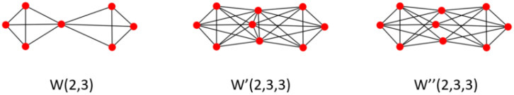 Figure 1
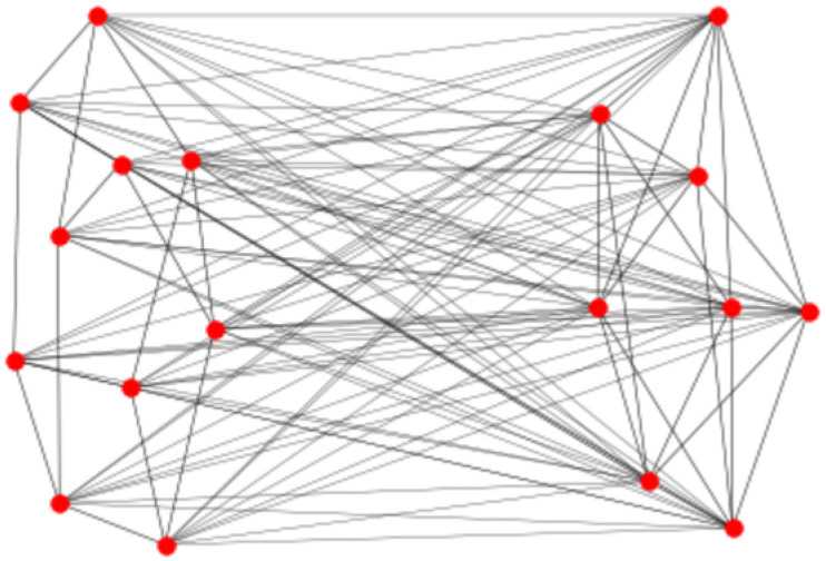 Figure 2
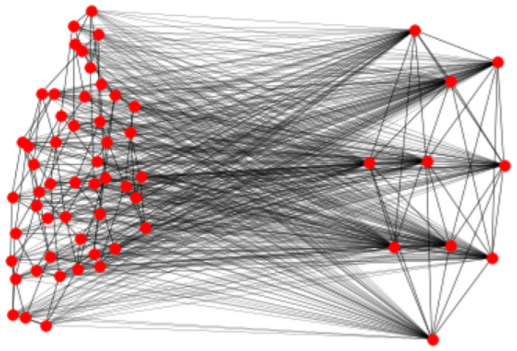 Figure 3
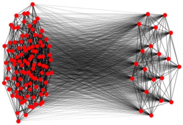 Figure 4
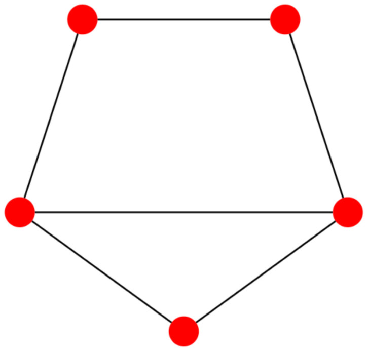 Figure 5
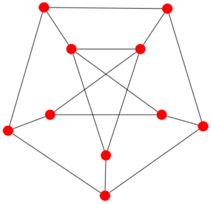 Figure 6
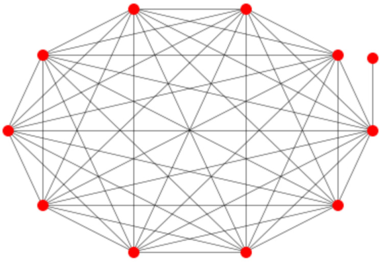 Figure 7
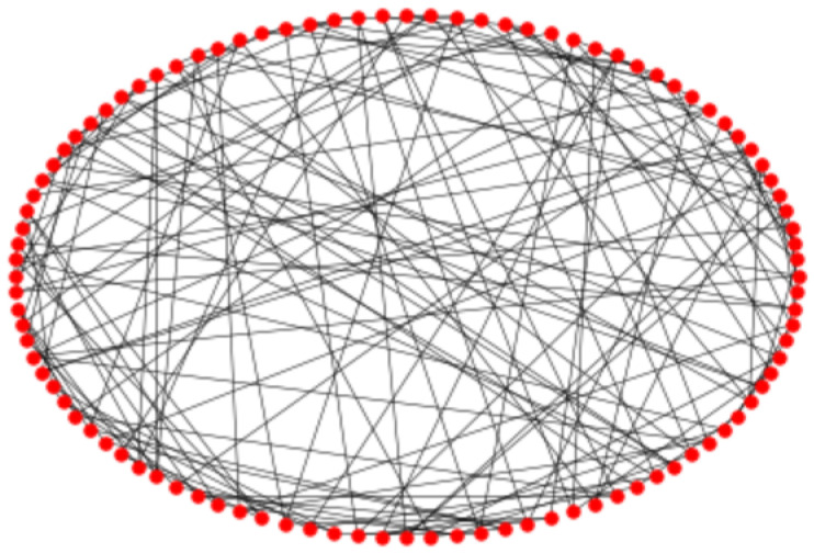 Figure 8
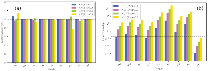 Figure 9
- —European Union’s Horizon 2020 research and innovation program
- —Marie Sklodowska-Curie
- —Dutch National Foundation
Peer Reviews
No public reviews on file for this paper yet. If you reviewed it on a platform where reviews are public (OpenReview, ICLR, NeurIPS, ICML), you can paste yours below so the community can read it here.
Videos
No videos yet. Explain this paper in a talk, walkthrough, or lecture? Add one.
Taxonomy
TopicsGraph theory and applications · Complex Network Analysis Techniques · Advanced Queuing Theory Analysis
1. Introduction
Kemeny’s constant, a graph metric first proposed in 1960 [1], links random walks, Markov chains, and spectral graph theory; see, for instance, [2,3,4].
An intuitive way to understand Kemeny’s constant is by random walks on a graph, which was also how it was originally presented by Kemeny [1]. For an undirected connected graph with an adjacency matrix A, we can define a transition matrix for the transition from state i to j, where is the degree of node i. This defines an irreducible finite-state Markov chain in discrete time with an transition matrix [5]. If we also know the mean first-passage time matrix denoting the average time to go from a vertex i to a vertex j (we take by convention), the Kemeny constant is defined by
where is the j-th component of the stationary solution of the random walk. The fact that does not depend on the index i, which can be interpreted as the starting state of the random walk and is therefore truly a constant, was discussed in a number of papers [6,7]. Hunter [8] and Kirkland [9] have analysed Relation (1) and established a connection with generalised matrix inverses.
The Kemeny constant also has an interpretation as a ‘mixing time’, which was originally proposed by Hunter in [7]. Here, we briefly repeat the demonstration that the Kemeny constant can be identified by a mixing time and show that this can be directly interpreted in terms of entropy. Let us define the ‘time to mixing’, T, of a Markov chain following [7], as the smallest index k at which , where Y is a random variable distributed according to the stationary distribution of the Markov chain . We can now calculate the conditional expectation value of T, ,
where is the mean first-passage time for going from node i to node j.
Expression Equation (2) for the mixing time permits an interpretation in terms of relative entropy or Kullback–Leiber divergence , which measures the distance between the distributions p and ; see also [10]. The relative entropy is defined as
Since with equality only when for all , the time to mixing can be interpreted as the smallest value of n for which the relative entropy .
Kemeny’s constant has recently also been suggested as a metric to identify bottleneck roads whose removal would greatly reduce the connectivity of the network [11] or as a metric to determine the ‘superspreader’ links that transmit disease between different communities [12].
It has already been established that there are several equivalent ways to express Kemeny’s constant: using effective graph resistance, random walks, spectral graph theory, and pseudo-inverse Laplacians; see [8].
The study of Kemeny’s constant is still an active and relevant research field, as was showcased by the mini-symposium “Kemeny’s constant on networks and its application”, which was organised as part of the 24th Conference of the International Linear Algebra Society, which took place in Galway, Ireland, 20–24 June 2022 [13] as well as recent papers addressing applications of Kemeny’s constant to different networks [14,15].
In 2017, Wang et al. [4] derived a closed-form formula for Kemeny’s constant, for a random walk on a graph G with N nodes and L edges, where the transition matrix was given by , where is the adjacency matrix of G and is a diagonal matrix containing the degrees of the nodes. In [4], it was shown that can be expressed in terms of the Moore–Penrose pseudo-inverse of the Laplacian matrix of G, as
where the column vector and denotes the degree vector for the graph.
In [4], not only Equation (3) was derived, but also a closely connected upper bound:
where is the average degree and is the largest eigenvalue of the Laplacian matrix corresponding to graph G. Here, denotes the diagonal matrix containing the degrees of the nodes. The heterogeneity index , measuring the variability in the degrees of the nodes (see [16]) is defined as
where is the degree of the i-th node.
It was shown in [17] that the upper bound given in Equation (4) is tight, meaning that we have an equality in Equation (4), for two classes of graphs, namely complete bipartite graphs and (generalised) windmill graphs. A windmill graph consists of copies of the complete graph , with each node connected to a common node. Two generalisations of windmill graphs were suggested by Kooij [18] in 2019. For both generalisations, we replace the central node, connecting all copies of the complete graph , with l central nodes. For the first generalisation, we assume that the l central nodes are all connected, i.e., they form a clique . We call this a generalised windmill graph of Type I and denote it by . For the second generalisation, we assume that the l central nodes have no connections among each other. We will refer to it as a Type II generalised windmill graph and denote it by . Figure 1 shows examples of a windmill graph and its two generalisations,
The aim of this paper is four-fold. First, we will consider a broad family of graphs, which contain complete bipartite and (generalised) windmill graphs as special cases, and show analytically that for these graphs, the bound Equation (4) is tight. Graphs in this family have in common that they are bimodal and have a diameter of two. However, we will also show that these conditions are not sufficient to ensure that Equation (4) is tight. Next, we compare the complexity of the computation of the upper-bound Equation (4) with the exact expression for Kemeny’s constant, given by Equation (3). In [17], we have already compared the exact value of with the upper bound for some real-world networks. However, the considered networks were of rather moderate size ( ). Here, we will assess the performance of on real-world networks of sizes up to around 365 K nodes and M edges.
Finally, in addition to Equation (4), we also assess the performance of an upper bound suggested by de Vriendt [19] based on the so-called resistance radius of a graph:
where the resistance radius is defined as
with denoting the resistance matrix and u the all-one vector. The upper-bound Equation (5) is tight for vertex-transitive graphs. Here, we remark that vertex-transitive graphs are rather exceptional and are typically highly symmetric; examples of vertex-transitive graphs are Cayley graphs and the Petersen graph [20]. We will show in this paper that the bound is not a good estimate for the Kemeny constant for the classes of graphs that are considered in this paper and that is in general a much better estimate.
2. A Family of Biregular Graphs with Diameter 2
2.1. Construction
The aim is to construct a family of graphs that contains the complete bipartite and (generalised) windmill graphs as special cases and is commonly known as the combination of two regular graphs, denoted . We start the construction by considering a -regular graph on nodes, and a -regular graph on nodes. We assume and also . Finally, we connect every node in to every node in to obtain the graph G. The nodes in G that are also in have degree , while the nodes in have degree . This construction yields a graph that is a so-called biregular graph in which all nodes of have the same degree and the same holds for all nodes of ; see also [21]. Only if is the graph G regular. By construction, G has diameter 2.
The choice of and leads to the complete bipartite graph . If we take isolated copies of the complete graph as and an isolated node for , then G is the windmill graph . If instead, we let be a complete graph , then G is a generalised windmill graph of Type I, , whereas if we let consist of l isolated nodes, G is a generalised windmill graph of Type II, .
Figure 2 shows an example of a graph that belongs to the suggested family of graphs. Here, , on the left side of the figure, is a random regular graph with , on nodes, while is a graph on nodes, where each node has degree . For the graph G, the nodes in have degree 11, while the nodes in have degree 15.
2.2. Tightness of the Upper Bound KU(G)
We will now show for the family of graphs proposed in the previous subsection that the upper-bound Equation (4) for Kemeny’s constant is tight.
Theorem 1. Consider two graphs and with all vertices in with degree and those in degree . If we connect each of the vertices in with all nodes of , then Kemeny’s constant for the resulting graph G is given by , that is, the upper-bound Equation (4) is tight.
Proof. First, we give expressions for the average degree D and the heterogeneity index H, which appear in the upper-bound Equation (4). Denoting the degrees of the nodes in G in and as and , respectively, we obtain
and
The average degree of G, , which we abbreviate for notational convenience to D, is defined by
The heterogeneity index , a metric which quantifies the variability of the degree distribution (see [16]), is defined as follows:
where denotes the degree of node i in graph G. Using the expressions for degrees and found in (7) and (8) and expression (9) for D, we obtain
We will now prove the statement by first calculating the Laplacian matrix Q for the graph G, which has the following special structure:
where is an all-one matrix, and the square matrices and are defined as
where , is the Laplacian of graph ( ), and denote the identity matrices of size and , respectively. The decomposition of Q into 4 blocks can be understood by realising that the upper right-hand block, , represents the links that exist between each vertex of and all the vertices of . Since Q is a Laplacian matrix, we have to ensure that all rows sum up to zero, which can be achieved by adding to each of the diagonal entries of the block in the upper left-hand corner, that is, the block should be as defined above. Analogously, we find that the lower left-hand and right-hand blocks should be equal to and , respectively.Two eigenvectors, and , can be found by inspection. , which corresponds to eigenvalue , and , which has entries equal to and entries equal to and corresponds to .Because the largest Laplacian eigenvalue is upper-bounded by N, the number of nodes in a graph (see [22]), we directly obtain that is the largest eigenvalue of Q. Combining this with Equations (9)–(11), we obtain
Since eigenvectors corresponding to different eigenvalues are all orthogonal and those corresponding to the same eigenvalues can be chosen to be orthogonal, due to the symmetry of Q, all eigenvectors that are not equal to or are subject to
which leads to
We next turn to the expression , where where is the i-th eigenvalue of Q and is the normalised eigenvector. The conditions for the eigenvectors (15) imply that all terms in the expression vanish except the term associated with . More precisely, we find that
where , so the first components all have degree and the remaining components have degree , which implies by Equation (15). Finally, because from , we obtain
it follows that equals Equation (14), which proves the proposition. □
2.3. Some Examples
As a first example, we consider the graph depicted in Figure 2, where , , and . Using Python (https://www.python.org/) code, we have evaluated both K and . For this network, we obtain , which is equal to to numerical precision, as should be according to Theorem 1. On the other hand, the upper bound based upon the resistance radius gives , which is reasonably close to the actual value.
Next, we consider a graph where , , and ; see Figure 3. Here, we get , and again, K and are numerically extremely close. On the other hand, for this graph, the bound Equation (5) is two orders larger than the actual value: .
As a final example, we consider the case where , , and ; see Figure 4. Now, and again K and are equal to numerical precision. Again, the bound based on the resistance radius is much higher: .
We end this subsection by noting that the choice for the examples in this subsection was rather arbitrary. We also ran our Python script on several other graphs with sizes up to 1500 nodes. Each time, it yielded the same result: K and have values that are numerically very close (see also [4,17] for more numerical comparisons), while the upper bound exceeds Kemeny’s constant by a few orders.
3. Graphs with Diameter 2 for Which KU(P) Is Not Tight
3.1. Bimodal Graphs with Diameter 2 for Which Equation (4) Is Not Tight
The numerical results of the examples on biregular graphs with diameter 2 from the previous section showed that in all these cases, the approximation of K by is actually exact. In other words, the bound is tight in these cases. Therefore, one might be tempted to believe that Equation (4) is tight for all biregular graphs with diameter 2. In this section, we prove that this is not the case by giving some counterexamples.
The simplest counterexample we could find consists of the cycle graph with an additional link; see Figure 5.
For this graph, we get , and . There is a simple procedure to check whether or not a biregular graph G with diameter 2 belongs to the graph family constructed in the previous section. First, partition the nodes into two sets and where all the nodes in the set have degree , while all the nodes in the set have degree . Next, verify if the number of links between the 2 sets is and all nodes of are linked to all nodes of . If this is not the case, the graph . In the other case, remove all links between the sets and . If the remaining two graphs are not both regular, then the original graph G does not belong to the family constructed in the previous section, that is,
The second counterexample is constructed by adding a link to the Petersen graph; see Figure 6.
For this graph, we get , and .
3.2. Non-Biregular Graphs with Diameter 2
We now give an example of a non-biregular graph with diameter 2, for which the upper-bound Equation (4) also does not equal Kemeny’s constant. We construct the graph by first taking a complete graph on N nodes. Next, we add one node and connect it to one node in and therefore the resulting graph has diameter 2. The resulting graph has nodes with degree , one node with degree N, and one node with degree 1. Figure 7 shows an example with .
Applying Equation (3), we get , while the upper bound of Equation (4) gives , while .
4. Regular Graphs
In this section, we consider regular graphs on N nodes with degree r. In this case, the relation between Kemeny’s constant and the effective graph resistance was shown [23] to be
where denotes the effective graph resistance. Next, we show that for these graphs, the upper-bound Equation (4) is also tight. For this, we will use the following expression for the effective graph resistance (see [4]):
For r-regular graphs, , and therefore Equation (4) gives
hence according to Equation (18).
As an example, we consider a random 3-regular graph on 100 nodes (see Figure 8), which has a diameter 10. We get numerically , which is indeed equal to up to the numerical precision of . Applying Equation (5) gives . In this case, the upper-bound Equation (5) is not tight because the graph is not vertex-transitive.
5. Complexity for the Computation of KU(P)
The time complexity of , computed via Equation (3), is dominated by the Laplacian pseudo-inverse, which is as expensive as performing a dense matrix multiplication and takes in practice with standard tools. On the other hand, the time complexity of mainly depends on two operations: computing the largest Laplacian eigenvalue and performing the dot product of a degree vector and the diagonal element vector of the Laplacian pseudo-inverse. Interestingly, to compute , we can avoid the full pseudo-inversion as it only requires the diagonal elements of the Laplacian pseudo-inverse. Algorithms that approximate the diagonal (or the trace) of matrices often use iterative methods, sparse direct methods [24], Monte Carlo [25] or deterministic probing techniques [26]. Although faster than computing the full inversion, these approaches are still time-consuming in practice for large graphs [27]. For that reason, we employ a recently proposed algorithm that approximates the diagonal entries of the Laplacian pseudo-inverse using combinatorial connections [27]. This algorithm exploits the relation between effective resistance and the pseudo-inverse Laplacian. In order to calculate the diagonal elements of , it is sufficient to compute the electrical farness of each node u in the set of all nodes V; the farness is defined by
Here, is the effective resistance between node u and v, which is the potential difference between u and v when a unit current is injected in graph G at node u and extracted at node v [28]. Rather than calculate for each pair of nodes, we sample a set of uniform spanning trees. This approach provides a probabilistic absolute approximation guarantee.
The algorithm’s time complexity is summarised in the following proposition:
Proposition 1([27]). Let be an undirected and weighted graph with N nodes and L edges. The sampling algorithm, briefly described above, gives an approximation of the diagonal elements of with absolute error with probability in an expected time , where is the length of the longest shortest path (eccentricity) starting in a selected node u. For small-world graphs and (for high probability), this yields a time complexity of .
For networks that have small-world characteristics, a common feature for many real-world networks [29], the above algorithm obtains a -approximation with high probability, in a time that is linear in L up to polylogarithmic terms and quadratic in . Furthermore, computing the largest Laplacian eigenvalue does not change the overall complexity bound. More precisely, this step often takes time for sparse matrices using standard iterative methods, such as the Lanczos algorithm [30]. In general, the actual running time for this step highly depends on the desired accuracy and the eigenvalue distribution of the involved matrix. Overall, the complexity bound for computing for small-world graphs using the above techniques is linear in the number of links L (up to a polylogarithmic factor).
6. Analysis of Some Large Real-World Networks
In this section, we analyse the performance of our proposed bound, , compared to Kemeny’s constant, , in terms of accuracy and running time results. For , our implementation uses the NetworKit [31] graph library to compute the diagonal elements of (via the algorithm of Angriman et al. [27]) and the Slepc library (https://slepc.upv.es/) (accessed on 2 December 2024) to compute the largest Laplacian eigenvalue. , in turn, is computed via Equation (3) and our implementation uses the Eigen library (http://eigen.tuxfamily.org) (accessed on 2 December 2024) to compute the entire pseudo-inverse, . We do not include any comparisons against since, computationally, it is as expensive as the exact computation of Kemeny’s constant. Our test machine is a shared-memory server with a 2x 18-Core Intel Xeon 6154 CPU and a total of 1.5 TB RAM. To ensure reproducibility, experiments are managed by SimexPal [32]. In Table 1, we list the real-world graphs that are used in our experiments, downloaded from SNAP [33] and NR [34] public repositories. In this context, we consider as medium graphs those whose vertex count is <57 K. The largest graph has around 365 K nodes and M edges.
For the medium graphs of Table 1, we are able to compare our bound relatively to Kemeny’s constant , and the results are illustrated in Figure 9. is computed with different error bounds ( ) for the approximation of the diagonal elements (via the algorithm of Angriman et al. [27])—they correspond to the respective numbers next to the names in Figure 9. Regarding the accuracy, we observe that our approach for computing is overall highly accurate for all values of and graphs. More precisely, on average (computed via geometric mean) over the medium-size graphs, our approach is 0.33% 0.27% 0.25% and 1.26% away from the exact Kemeny’s constant for and , respectively. Meanwhile, the running time is on average and 141× faster than the exact computation for each , respectively. Figure 9a shows that on individual graphs, a larger value ( ) may result in a slightly less accurate bound—up to 10% away from the exact value (arx). Moreover, in Figure 9b, we observe that for the inf graph, computing the exact Kemeny’s constant is much faster than computing via Algorithm [27]. The primary reason for that is the small size (6K edges) for which an exact computation of the entire pseudo-inverse is still fast enough. A second reason for the slow performance of the algorithm of Angriman et al. could be due to the high diameter of the graph in question (≫ ).
In Table 2, we illustrate our results for the largest graphs of Table 1. For this experiment, we set for the approximation of the diagonal elements of as this offers the best trade-off between accuracy and speed, according to the previous experiment. Unfortunately, we were not able to compute exact values for Kemeny’s constant for these graphs, as all involved runs timed out at 18,000 s. This is due to the prohibitive time and space complexity of the pseudo-inversion operation required by .
7. Conclusions
We have investigated Kemeny’s constant for a number of networks using the exact expression from [4] and compared this expression with two upper bounds: one that was derived in Ref. [19] and is known to be tight for vertex-transitive graphs, and the other bound was derived in [4] and is written in terms of degrees of the nodes, the diagonal elements of the pseudo-inverse Laplacian, the largest eigenvalue of the Laplacian matrix and the heterogeneity of the degrees of the nodes.
We have numerically demonstrated that the bound is generally a much better approximation for than for the networks that we have explored. Moreover, we have proved that for any graph G composed of two regular graphs and with all nodes of the graph connected to each node of , the bound is tight. This generalises earlier findings that the bound is tight for (generalised) windmill and complete bipartite graphs.
As an illustration of the advantages of using the expression to estimate the Kemeny constant, we numerically calculated the Kemeny constant for a number of real-world large networks. We find that the calculation of can be performed very efficiently, displaying efficiency gains in the order of a factor 100–1000, for networks up to 57 K nodes. The upper bound can still be obtained in a reasonable time for networks up to 365 K nodes.
The reference list from the paper itself. Each links out to its DOI / PubMed record.
- 1Kemeny J.G. Snell J.L. Finite Markov Chains D. Van Nostrand Princeton, NJ, USA 1960
- 2Lovász L. Random Walks on Graphs: A Survey Paul Erdös is Eighty Bolyai Society, Mathematical Studies Keszthely, Hungary 1993 Volume 2146
- 3Palacios J.L. Renom J.M. Bounds for the Kirchhoff index of regular graphs via the spectra of their random walks Int. J. Quantum Chem.20101101637164110.1002/qua.22323 · doi ↗
- 4Wang X. Dubbeldam J.L.A. Van Mieghem P. Kemeny’s constant and the effective graph resistance Linear Algebra Its Appl.2017535231244
- 5Noh J.D. Rieger H. Random Walks on Complex Networks Phys. Rev. Lett.20049211870110.1103/Phys Rev Lett.92.11870115089179 · doi ↗ · pubmed ↗
- 6Levene M. Loizou G. Kemeny’s Constant and the Random Surfer Am. Math. Mon.200210974174510.1080/00029890.2002.11919905 · doi ↗
- 7Hunter J. Mixing times with applications to perturbed Markov chains Linear Algebra Its Appl.200641710812310.1016/j.laa.2006.02.008 · doi ↗
- 8Hunter J.J. The role of Kemeny’s constant in properties of Markov chains Commun. Stat.-Theory Methods 20144313091321