A convexity‐constrained parameterization of the random effects generalized partial credit model
David J. Hessen

TL;DR
This paper introduces a new mathematical approach to improve the estimation of parameters in a statistical model used for scoring items.
Contribution
The novel contribution is a convexity-constrained parameterization that ensures proper maximum likelihood estimation.
Findings
A closed-form expression using a cumulant generating function is introduced.
The convexity constraints ensure a single global maximum in the likelihood function.
The method is demonstrated with an example and includes goodness-of-fit testing.
Abstract
An alternative closed‐form expression for the marginal joint probability distribution of item scores under the random effects generalized partial credit model is presented. The closed‐form expression involves a cumulant generating function and is therefore subjected to convexity constraints. As a consequence, complicated moment inequalities are taken into account in maximum likelihood estimation of the parameters of the model, so that the estimation solution is always proper. Another important favorable consequence is that the likelihood function has a single local extreme point, the global maximum. Furthermore, attention is paid to expected a posteriori person parameter estimation, generalizations of the model, and testing the goodness‐of‐fit of the model. Procedures proposed are demonstrated in an illustrative example.
Genes, proteins, chemicals, diseases, species, mutations and cell lines named across the full text — each resolved to its canonical identifier and authoritative record.
Click any figure to enlarge with its caption.
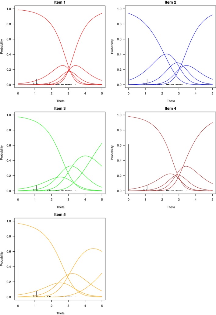 FIGURE 1
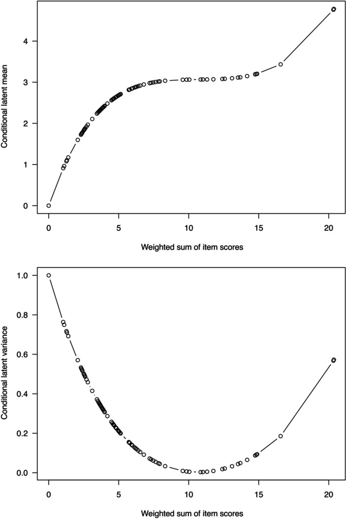 FIGURE 2
| 302 | 0.000 | 1.000 | 1 | 2.711 | 0.199 | 1 | 3.068 | 0.005 | |||
| 7 | 1.172 | 0.692 | 1 | 2.919 | 0.105 | 1 | 3.113 | 0.044 | |||
| 1 | 1.968 | 0.459 | 1 | 3.020 | 0.045 | 5 | 1.599 | 0.570 | |||
| 1 | 2.482 | 0.287 | 1 | 3.016 | 0.048 | 1 | 2.996 | 0.061 | |||
| 37 | 1.106 | 0.710 | 1 | 2.670 | 0.216 | 2 | 2.852 | 0.138 | |||
| 5 | 1.924 | 0.473 | 1 | 3.006 | 0.055 | 1 | 2.562 | 0.258 | |||
| 7 | 1.878 | 0.487 | 1 | 3.063 | 0.005 | 1 | 2.824 | 0.151 | |||
| 1 | 2.426 | 0.307 | 1 | 2.704 | 0.202 | 1 | 3.121 | 0.049 | |||
| 1 | 2.945 | 0.091 | 1 | 2.882 | 0.124 | 1 | 3.205 | 0.093 | |||
| 1 | 2.396 | 0.318 | 1 | 3.149 | 0.065 | 1 | 2.602 | 0.243 | |||
| 7 | 0.962 | 0.750 | 12 | 0.910 | 0.764 | 2 | 2.818 | 0.153 | |||
| 1 | 1.828 | 0.502 | 3 | 1.744 | 0.527 | 1 | 3.062 | 0.006 | |||
| 6 | 1.779 | 0.517 | 1 | 2.341 | 0.337 | 1 | 3.193 | 0.088 | |||
| 1 | 2.363 | 0.329 | 1 | 2.308 | 0.348 | 1 | 2.593 | 0.246 | |||
| 2 | 2.332 | 0.340 | 1 | 2.691 | 0.208 | 1 | 2.842 | 0.143 | |||
| 1 | 2.296 | 0.352 | 1 | 2.237 | 0.372 | 1 | 2.979 | 0.072 | |||
| 5 | 2.262 | 0.364 | 1 | 2.579 | 0.251 | 1 | 3.035 | 0.033 | |||
| 3 | 2.642 | 0.227 | 1 | 1.725 | 0.533 | 1 | 3.097 | 0.033 | |||
| 1 | 2.986 | 0.068 | 1 | 2.683 | 0.211 | 1 | 3.066 | 0.003 | |||
| 1 | 2.814 | 0.155 | 1 | 2.905 | 0.112 | 1 | 3.202 | 0.092 | |||
| 11 | 1.080 | 0.717 | 1 | 3.067 | 0.004 | 1 | 3.193 | 0.088 | |||
| 5 | 1.861 | 0.492 | 1 | 2.284 | 0.356 | 1 | 2.106 | 0.415 | |||
| 1 | 2.415 | 0.311 | 1 | 2.889 | 0.120 | 1 | 3.080 | 0.018 | |||
| 2 | 2.385 | 0.322 | 1 | 3.071 | 0.009 | 1 | 3.060 | 0.009 | |||
| 1 | 1.761 | 0.522 | 1 | 2.610 | 0.239 | 1 | 3.434 | 0.186 | |||
| 2 | 2.320 | 0.344 | 1 | 3.083 | 0.021 | 1 | 4.782 | 0.573 | |||
| 1 | 2.634 | 0.230 | 1 | 2.647 | 0.225 | 1 | 4.762 | 0.568 | |||
| 2 | 1.844 | 0.497 | 2 | 2.873 | 0.128 | ||||||
| 1 | 2.374 | 0.326 | 1 | 3.193 | 0.088 |
| Parameter | Estimate | SE | Parameter | Estimate | SE | Parameter | Estimate | SE |
|---|---|---|---|---|---|---|---|---|
| −4.340 | 0.521 | 3.107 | 0.284 | 3.107 | 0.284 | |||
| −8.705 | 1.440 | 3.125 | 0.369 | 3.116 | 0.210 | |||
| −12.851 | 2.246 | 2.968 | 0.488 | 3.067 | 0.182 | |||
| −17.020 | 3.142 | 2.984 | 0.651 | 3.046 | 0.192 | |||
| −2.781 | 0.343 | 2.136 | 0.165 | 2.136 | 0.165 | |||
| −6.514 | 1.026 | 2.868 | 0.188 | 2.502 | 0.106 | |||
| −10.768 | 1.777 | 3.267 | 0.359 | 2.757 | 0.135 | |||
| −14.717 | 2.689 | 3.033 | 0.496 | 2.826 | 0.131 | |||
| −3.738 | 0.416 | 3.383 | 0.374 | 3.383 | 0.374 | |||
| −6.293 | 1.147 | 2.312 | 0.384 | 2.847 | 0.177 | |||
| −9.868 | 2.002 | 3.236 | 0.604 | 2.977 | 0.220 | |||
| −14.733 | 3.210 | 4.403 | 1.601 | 3.333 | 0.386 | |||
| −3.905 | 0.396 | 3.083 | 0.302 | 3.083 | 0.302 | |||
| −7.433 | 1.079 | 2.785 | 0.283 | 2.934 | 0.168 | |||
| −10.997 | 1.774 | 2.813 | 0.416 | 2.894 | 0.162 | |||
| −15.083 | 2.589 | 3.226 | 0.528 | 2.977 | 0.162 | |||
| −3.544 | 0.315 | 3.418 | 0.362 | 3.418 | 0.362 | |||
| −6.030 | 0.818 | 2.397 | 0.330 | 2.907 | 0.187 | |||
| −9.198 | 1.385 | 3.055 | 0.704 | 2.957 | 0.241 | |||
| −15.030 | 2.833 | 5.625 | 1.870 | 3.624 | 0.451 | |||
| 1.397 | 0.259 | −0.251 | 0.020 | |||||
| 1.302 | 0.228 | 0.046 | 0.011 | |||||
| 1.105 | 0.215 | −0.006 | 0.003 | |||||
| 1.267 | 0.217 | 0.001 | 0.000 | |||||
| 1.037 | 0.169 | |||||||
| −0.110 | 0.019 | |||||||
| 0.005 | 0.002 | |||||||
| −0.074 | 0.005 |
Peer Reviews
No public reviews on file for this paper yet. If you reviewed it on a platform where reviews are public (OpenReview, ICLR, NeurIPS, ICML), you can paste yours below so the community can read it here.
Videos
No videos yet. Explain this paper in a talk, walkthrough, or lecture? Add one.
Taxonomy
TopicsPsychometric Methodologies and Testing · Statistical Methods and Bayesian Inference · Statistical Methods and Inference
INTRODUCTION
1
A well‐known item response model for the measurement of a single latent variable by a set of polytomously scored items with ordered response categories is the generalized partial credit model (Muraki, 1992, 1993). In the generalized partial credit model, the conditional probability distribution of an item score given the latent variable is assumed to depend on the latent variable, an item scaling parameter, and item category location parameters. Well‐known special cases of the generalized partial credit model are the partial credit model (Agresti, 1993; Masters, 1982) and the rating scale model (Andrich, 1978). In the case of dichotomously scored items, the generalized partial credit model equals the two‐parameter logistic model (Birnbaum, 1968) and includes the Rasch model (Rasch, 1960, 1966) as a special case. Generalizations of the generalized partial credit model are the two‐parameter partial credit model (Hemker et al., 1996) and the nominal response model (Bock, 1972).
A distinction can be made between the fixed effects and the random effects generalized partial credit model. In the fixed effects generalized partial credit model, item and person parameters are treated as fixed and can be jointly estimated. Unfortunately, however, joint maximum likelihood estimators of item parameters have been shown to be inconsistent if the number of items is fixed and the number of examinees tends to infinity (Andersen, 1971, 1973; Haberman, 1977). In the random effects generalized partial credit model, the latent variable is assumed to be a random variable with a distribution in the population of examinees and the examinees in the sample are assumed to be randomly sampled from the population. Usually, the latent variable is assumed to have a specific distribution in the population of examinees, and if the generalized partial credit model and the assumed latent variable distribution are true, then item parameters can consistently be estimated in the joint marginal probability distribution of the item scores, where the latent variable has been integrating out.
For the random effects generalized partial credit model without a specified latent variable distribution, it has been shown that the joint marginal probability distribution of the item scores has a closed‐form expression (Hessen, 2021). This closed‐form expression does not seem useful for fitting the random effects generalized partial credit model because of complicated inequality constraints that follow from moment inequalities. However, due to this closed‐form expression, an extended version of the model (Cressie & Holland, 1983; Tjur, 1982) can be fitted to data without requiring the specification of a population distribution for the latent variable and without using numerical integration techniques. An important advantage of using the closed‐form expression in practice is that there will be no estimation bias due to a misspecification of the population distribution of the latent variable. Another advantage is that the model cannot be incorrectly rejected due to a violation of the assumed latent variable distribution. Despite these advantages, the use of this closed‐form expression in fitting the extended generalized partial credit model does not guarantee a solution that is consistent with a latent random variable. Due to ignoring moment inequalities, the estimation solution might not be proper (Cressie & Holland, 1983). Another disadvantage is that in maximum likelihood estimation of the parameters of the extended model, the likelihood function might have several local extreme points.
In this paper, an alternative closed‐form expression of the random effects generalized partial credit model is presented. It is shown that the joint marginal probability distribution of the item scores under the random effects generalized partial model has a closed‐form expression in terms of item category location parameters, item scaling parameters, and an incomplete conditional cumulant‐generating function of the latent random variable given an arbitrary reference score pattern. Since the incomplete cumulant‐generating function is a convex polynomial, the random effects generalized partial credit model can now be fitted to data using this alternative closed‐form expression and appropriate convexity constraints. Fitting the model in this way is latent variable distribution‐free, takes moment inequalities into account, and guarantees a proper estimation solution. Moreover, due to the convexity constraints, the likelihood function now has a single local extreme point, the global maximum.
The framework in which the new closed‐form expression is derived allows the fitting of the random effects generalized partial credit model in a subpopulation defined by a subset of the support of the joint probability distribution of the item scores in the total population (Hessen, 2023). The possibility of fitting a subpopulation model instead of the population model greatly enhances the number of applications in practice because the subpopulation can be chosen so that the normalizing constant in the model expression can efficiently be calculated. For example, if the subpopulation is defined by the set of all observed score patterns, then even when the number of items is large, the number of addends in the denominator of the normalizing constant cannot exceed the sample size. Thus, within this framework, the latent variable distribution‐free application of the random effects generalized partial credit model is not restricted by the number of items.
The remainder of this paper is organized as follows. In the following section, an alternative closed‐form expression of the probability distribution of the item scores under the random effects generalized partial credit model is derived. In the third section, the alternative closed‐form expression is subjected to convexity constraints. In the fourth section, maximum likelihood estimation of the parameters of the random effects generalized partial credit model is discussed. In the fifth section, attention is paid to goodness‐of‐fit testing and to more general models that can be used as alternative models in likelihood ratio tests. One of these more general models is shown to be a convexity‐constrained parameterization of the random effects nominal response model. The sixth section is devoted to expected a posteriori (EAP) estimation of person parameters and to estimating cumulants (e.g., mean, variance, skewness, kurtosis) of the latent variable in the total (sub)population. In the seventh section, an illustrative example is given in which both the distribution of EAP estimates of person parameters and estimates of cumulants in the total (sub)population seem to indicate that the latent variable distribution in the (sub)population is positively skewed and platykurtic.
A CLOSED‐FORM MODEL EXPRESSION
2
Consider a situation in which a test of k polytomously scored items is administered to a sample of examinees. The number of response categories of item i is denoted by mi+1, where mi≥1, for all i, and is not restricted to be the same for all i. It is assumed that the examinees are randomly sampled from an infinite population. It is also assumed that the items are measures of a single latent random variable Θ with realization θ. Next, let Y=(Y1,…,Yk)′ be the random vector of item scores, and let y=(y1,…,yk)′ be a realization, where yi∈{0,1,…,mi}, for i∈{1,2,…,k}. The joint marginal probability distribution of Y can be written
where P(Y=y|θ) is the joint conditional probability distribution of Y given Θ=θ, and f(θ) is the probability density of Θ in the population of examinees. The elements of Y are assumed to be conditionally independent given Θ=θ. The conditional independence of the elements of Y given Θ=θ is defined as
where P(Yi=yi|θ) is the conditional probability distribution of Yi given Θ=θ. Using dummy scores xis=1 if yi=s and xis=0 otherwise, for s∈{1,…,mi}, the conditional probability distribution of Yi given Θ=θ can be written
where Vis(θ)=P(Yi=s|θ)/P(Yi=0|θ) is the odds of score s on item i relative to score 0 on item i as a function of θ and P(Yi=0|θ)=1+∑s=1miVis(θ)−1. The use of the dummy scores in this way fixes the reference category for each item score. The model framework of interest, however, requires flexibility in choosing a different reference category for each item score. By what now follows, this flexibility is obtained. From Eq. 3 it follows for fixed item score y0i that
where x0is=1 if y0i=s and x0is=0 otherwise, for s=1,…,mi. Solving for P(Yi=0|θ) from Eq. 4 and substitution into Eq. 3 yields
where x˜is=xis−x0is. Next, substitution from Eqs. 2 and 5 into Eq. 1 yields
where P(Y=y0|θ)=∏i=1kP(Yi=y0i|θ). Note that
where Via(θ)=P(Yi=a|θ)/P(Yi=a−1|θ) is the odds of score a on item i relative to score a−1 on item i as a function of θ.
In the generalized partial credit model (Muraki, 1992, 1993) it is assumed that
where αi is an item scaling parameter and δia is an item category location parameter that gives the threshold θ value for which P(Yi=a−1|θ)=P(Yi=a|θ). Substitution from Eq. 8 into Eq. 7 yields
where ωis=∑a=1sδia/s is a transformed item category location parameter. The generalized partial credit model specializes to the partial credit model if αi=α, for all i (Masters, 1982). In the case of dichotomously scored items, that is mi=1, for all i, the generalized partial credit model equals the two‐parameter logistic model (Birnbaum, 1968) and the partial credit model equals the one‐parameter logistic model (Rasch, 1960, 1966).
Now, substitution from Eq. 9 into Eq. 6 gives, after some algebra,
where βis=−αisωis=−αi∑a=1sδia is another transformed item category location parameter, and y˜i=yi−y0i. If it is assumed that f(θ) is the standard normal density, then the integral in Eq. 10 is intractable but can numerically be approximated for any set of parameter values using Gaussian quadrature (Bock & Aitkin, 1981; Bock & Lieberman, 1970). The resulting random effects generalized partial credit model then has ∑i=1kmi+k free parameters. Here, however, no specific density is assumed for f(θ). Following Cressie and Holland (1983), we can write
where βi=(βi1,…,βimi)′, x˜i=(x˜i1,…,x˜imi)′, α=(α1,…,αk)′, y˜=(y˜1,…,y˜k)′, and g(θ|y0)=P(Y=y0|θ)f(θ)/P(Y=y0) is the conditional density of Θ given Y=y0. Note that under the partial credit model, α′y˜=αy˜, where y˜=∑i=1ky˜i. Subsequently, Eq. 11 can alternatively be written
where β=vec(β1,…,βk), x˜=vec(x˜1,…,x˜k), and MΘ|y0(α′y˜)=E{exp(α′y˜Θ)|y0} is the conditional moment‐generating function of Θ given Y=y0. It is well known that
where KΘ|y0(α′y˜) is the conditional cumulant‐generating function of Θ given Y=y0, and κr is the rth cumulant of Θ given Y=y0. The first cumulant κ1 is the conditional mean of Θ given Y=y0, the second cumulant κ2 is the conditional variance of Θ given Y=y0, and the third cumulant κ3 is the third central moment of Θ given Y=y0. Note that κ3 determines the skewness of the conditional distribution of Θ given Y=y0 because if κ3<0, then the coefficient of skewness given by κ3/κ23/2 is negative and the distribution is skewed to the left, and if κ3>0, the coefficient of skewness is positive and the distribution is skewed to the right. Also note that κ4 determines the kurtosis of the distribution of Θ given Y=y0 because if κ4<0, then the coefficient of kurtosis given by 3+κ4/κ22 is less than 3 and the distribution is platykurtic; if κ4=0, then the coefficient of kurtosis is 3 and the distribution is mesokurtic; and if κ4>0, then the coefficient of kurtosis is greater than 3 and the distribution is leptokurtic.
Substitution from Eq. 13 into Eq. 11 yields an unidentifiable model with infinitely many parameters. Hessen (2021) has shown, however, that the conditional moment‐generating function of Θ given Y=0 has a closed‐form expression in terms of common assocation parameters. Although this closed‐form expression yields an identifiable model after fixing the scale of θ, the expression is quite complex and its parameters are not very informative about the conditional distribution of Θ given Y=0. The result in the following theorem provides a closed‐form expression for the conditional moment‐generating function of Θ given Y=y0. This closed‐form expression for MΘ|y0(α′y˜) is simpler and better interpretable than the closed‐form expression for MΘ|0(α′y) proposed by Hessen (2021) and also yields an identifiable model.
Theorem 1Under the model in Eq. 12, the conditional moment‐generating function of Θ given Y=y0 equals
where λ1,…,λv−1 are the first v−1 conditional cumulants of Θ given Y=y0, and λv=KΘ|y0(v)(ξv) is the vth derivative of KΘ|y0(α′y˜)=lnMΘ|y0(α′y˜) for some real number ξv between zero and α′y˜.
The (v−1)th‐order Maclaurin polynomial of KΘ|y0(α′y˜) is
where KΘ|y0(r)(0) is the rth derivative of KΘ|y0(α′y˜) at α′y˜=0. The Lagrange form of the remainder is given by
for some real number ξv between zero and α′y˜. Solving Eq. 16 for KΘ|y0(α′y˜) and substitution into Eq. 13 yields Eq. 14, where λr=κr, for r=1,…,v−1, and λv=KΘ|y0(v)(ξv). This completes the proof. □
Note that v is a positive integer that must be specified. If v>2, then the moment‐generating function in Eq. 14 is incomplete and can only generate the first v−1 cumulants. In the case v=1 or λr=0, for r≥2, the distribution of Θ given Y=y0 is degenerate and the model equals the independence model. The special case in the following theorem is a reparameterization of the conditional normal generalized partial credit model (Hessen, 2021). In this special case, v=2 and λ2>0.
Theorem 2If all conditional cumulants given Y=y0 of order r>2 are zero, then the conditional distribution of Θ given Y=y is normal with mean κ1+κ2α′y˜ (linear) and variance κ2 (homoscedastic).
If κr=0, for r>2, then
which is the moment‐generating function of a normal random variable with mean κ1 and variance κ2. Furthermore,
where g(θ|y0)=(2πκ2)−1/2exp{−12(θ−κ1)2/κ2}, so that after some algebra it follows that
which can be recognized as a normal density with mean κ1+κ2α′y˜ and variance κ2. □
Substitution from Eq. 14 into Eq. 12 gives
where τ=P(Y=y0) is a normalizing constant. This normalizing constant equals
where S={y|P(Y=y)>0} is the support of Y, that is, the set of all score patterns that are observable. Without additional constraints the model is not identifiable. In the case v≥2, there are two indeterminacies. To show these two indeterminacies, the exponent on the right‐hand side of Eq. 18 is rewritten as ∑i=1k∑s=1mi(βis+λ1αis)x˜is+∑r=2vλr1r!(α′y˜)r. It follows that if βis=βis∗+cαis and λ1=λ1∗−c, for some constant c, then βis+λ1αis=βis∗+λ1∗αis. In addition, if α=α∗c−1 and λr=λr∗cr, for some constant c, then (y˜′α)rλr=(y˜′α∗)rλr∗. The two indeterminacies can be solved by arbitrarily setting λ1=0 and λ2=1. Consequently, the number of free parameters is ∑i=1kmi+k+v−2, for v≥2, and since λv is not a cumulant, only v−3 of the free parameters are conditional cumulants, for v≥3. Note that sign indeterminacy remains because (y˜′α)rλr=(y˜′α)r(−1)r·−λr, for odd r. In the random effects partial credit model, the right‐hand side of Eq. 18 equals ∑i=1k∑s=1miϕisx˜is+∑r=2vψr1r!y˜r, where ϕis=βis+λ1αs, for all i and s, and ψr=λrαr, for r=2,…,v, are identifiable. In this model, the number of free parameters is ∑i=1kmi+v−1.
CONVEXITY CONSTRAINTS
3
It follows from Hölder's inequality that the cumulant‐generating function KΘ|y0(α′y˜)=∑r=1vλr1r!(α′y˜)r is a convex polynomial. This polynomial is of degree v and has v coefficients. Consequently, its first derivative
is a strictly increasing polynomial of degree v−1, also with v coefficients, and its second derivative
is a non‐negative polynomial of degree v−2, with v−1 coefficients. It is well known that KΘ|y0(2)(α′y˜) is non‐negative on (−∞,∞) if and only if v−2=2q, where v is even, and
where p1(α′y˜) and p2(α′y˜) are polynomials whose degrees are at most q∈{0,1,2,…} (Brickman & Steinberg, 1962; Murray et al., 2016). If both polynomials are of degree q and each has q+1 coefficients, then the 2q+1 coefficients of the resulting polynomial of degree 2q in Eq. 22 are functions of 2q+2 parameters. Here, p1(α′y˜) and p2(α′y˜) should be chosen so that the coefficients of the resulting polynomial are functions of at most v−2=2q free parameters. Thus, at least two constraints are needed for identification.
Let p1(α′y˜)=ϵ1′t and p2(α′y˜)=ϵ2′t, where ϵ1=(ϵ10,ϵ11,…,ϵ1q)′, ϵ2=(ϵ20,ϵ21,…,ϵ2q)′, and t=1,α′y˜,(α′y˜)2,…,(α′y˜)q′. Then, KΘ|y0(2)(α′y˜)=(ϵ1′t)2+(ϵ2′t)2 equals
where hc(ϵ1,ϵ2)=∑j+j′=c(ϵ1jϵ1j′+ϵ2jϵ2j′)=1c!λc+2=1(r−2)!λr. As a consequence, we can write
and the cumulant‐generating function can be written
where λ1 is set to zero for identification. If, in addition, (ϵ10,ϵ20) is arbitrarily set to 12,12 or 35,45, then h0(ϵ1,ϵ2)=ϵ102+ϵ202=λ2=1, and the model is identified. More constraints can be added, however, while keeping the polynomial in Eq. 22 of degree 2q. If more constraints are added, then λ3,…,λv are modeled by a smaller number of parameters than v−2. For example, if the degree of p1(α′y˜) is q and the degree of p2(α′y˜) is q−1, then the degree of the resulting polynomial in Eq. 22 is still 2q, but its 2q+1 coefficients are now functions of 2q+1 parameters, of which only 2q−1 are free. Note that the elements of the parameter vectors ϵ1 and ϵ2 do not have a statistically meaningful interpretation. These elements should be conceived of as auxiliary parameters that are used only to constrain λ2,…,λv such that the conditional cumulant‐generating function of Θ given Y=y0 is convex.
MAXIMUM LIKELIHOOD ESTIMATION
4
The random effects generalized partial credit model given by
where KΘ|y0(α′y˜) is given by Eq. 29, is the population model for which the normalizing constant equals
where S is the support of Y. S might be an unknown proper subset of the set of all theoretically possible score patterns. Note that it follows from Eq. 12 that y0 must be an element of S; otherwise, the model is degenerate. Let O⊆B⊆S, where O is the set of all observed score patterns in the sample. Thus, selecting y0∈O guarantees that y0∈S. According to Hessen (2023), it follows from the population model in Eq. 30 that
where
Now, let ny be the number of examinees in the sample with score pattern y, for all y. Then, taking all possible score patterns into account and assuming the independence of observations, the likelihood function for the subpopulation model in Eq. 32 is given by
where n is the total sample size, and n˜=∑ynyx˜. For fixed α and without convexity constraints, the likelihood function for the model in Eq. 18 is log‐concave in the remaining parameters because for fixed α, the model is a member of the exponential family. Now, since KΘ|y0(α′y˜) is convex in α′y˜ and therefore also convex in α, the likelihood function in Eq. 34 is log‐concave in all parameters. This means that the likelihood function has a single local extreme point, the global maximum. To find the estimates of the elements of β, α, ϵ1, and ϵ2 that maximize the likelihood function in Eq. 34, the log‐likelihood function can be maximized with respect to the parameters subject to identification constraints using the Broyden‐Fletcher‐Goldfarb‐Shanno (BFGS) algorithm (Fletcher, 1987). The BFGS algorithm is a quasi‐Newton method in which the Hessian matrix of second derivatives is approximated using updates specified by (approximate) evaluations of the first derivatives. The first derivatives of the log‐likelihood function with respect to β, α, and the elements of ϵ1 and ϵ2 are given in Appendix.
Let β^i and α^i be the maximum likelihood estimates of βi and αi, respectively, for all i. Then the maximum likelihood estimate of the threshold vector δi=(δi1,…,δimi)′ is δ^i=−α^i−1Ji−1β^i, for all i, where Ji is a lower triangular matrix whose diagonal entries and entries below the main diagonal are all one, for all i. Let ϵ^1 and ϵ^2 be the maximum likelihood estimates of ϵ1 and ϵ2, respectively. Then the maximum likelihood estimate of λr is λ^r=hr−2(ϵ^1,ϵ^2)(r−2)!, for r∈{2,…,v}.
PERSON AND POPULATION PARAMETERS
5
A popular way of obtaining person parameter estimates under a random effects item response model is the calculation of the so‐called EAP estimates. An EAP estimate is an estimate of the conditional latent mean given score pattern y. The calculation of such an estimate requires a theoretical expression for the conditional latent mean given score pattern y. The theoretical expression of this conditional latent mean can be obtained via the moment‐generating function of the latent variable given score pattern y. This conditional moment‐generating function is given in the following theorem.
Theorem 3Under the random effects generalized partial credit response model, the conditional moment‐generating function of Θ given Y=y is
The conditional moment‐generating function of Θ given Y=y is given by
Substitution from Eq. 17 into Eq. 36 yields
and factorizing ∑r=1v(r!)−1 gives Eq. 35. □
The jth derivative of KΘ|y(z)=lnMΘ|y(z) with respect to z can be shown to be equal to
Consequently, the jth conditional cumulant of Θ given Y=y is given by
KΘ|y(1)(0)=μy and KΘ|y(2)(0)=σy2 are the conditional mean and variance of Θ given Y=y, respectively. Note that since μy is exactly equal to KΘ|y0(1)(α′y˜) in Eq. 20, it is a strictly increasing function of α′y˜. Also note that since σy2 is exactly equal to KΘ|y0(2)(α′y˜) in Eq. 21, it is a non‐negative function of α′y˜. The maximum likelihood estimate of the jth conditional cumulant of Θ given Y=y is given by
where λ^r is as before and α^ is the maximum likelihood estimate of α. The maximum likelihood estimate of μy is the EAP person parameter estimate given by κ^1y=μ^y, for all y. The maximum likelihood estimate of σy2 is κ^2y=σ^y2, for all y.
It is well known that the jth conditional non‐central moment E(Θj|y)=μjy′ is a jth‐degree polynomial in the first j conditional cumulants of Θ given Y=y. The first four conditional non‐central moments as polynomial functions of the first four conditional cumulants are given in Appendix. By the law of total expectation, it then follows that the jth non‐central moment of Θ in the total population defined by B is given by
Then the first four cumulants of Θ (mean, variance, skewness, and kurtosis) in the population defined by B are given by
respectively. Thus, with the maximum likelihood estimates of the first four conditional cumulants of Θ given Y=y, for all y∈B, maximum likelihood estimates of the first four conditional non‐central moments of Θ given Y=y can be calculated, for all y∈B. Subsequently, the maximum likelihood estimates of the first four non‐central moments of Θ in the population defined by B can be calculated using Eq. 39 and, finally, the maximum likelihood estimates of the first four cumulants of Θ in the population defined by B.
GOODNESS OF FIT AND GENERALIZATIONS
6
For assessing the goodness of fit of a random effects generalized partial credit model in the subpopulation defined by B⊇O, Pearson's asymptotic chi‐squared test or the likelihood ratio test against the saturated model might be appropriate. However, these tests often cannot be validly applied due to too many observed score patterns with low sample frequencies. Better goodness‐of‐fit tests in these circumstances are the alternative likelihood ratio tests proposed by Hessen (2023).
In addition, a random effects generalized partial credit model can be tested against less general alternatives than the saturated model using likelihood ratio tests. One such less general alternative is the model given by
This model specializes to the random effects generalized partial credit model if νis=βis+λ1αis+12λ2αi2s2, ρij=λ2αiαj, and λr=hr−2(ϵ1,ϵ2)(r−2)!, for r≥2. Another less general alternative is the random effects nominal response model (Bock, 1972) given by
where η is a vector of unrestricted item category scaling parameters. Note that if η′x˜=∑i=1k∑s=1miηisxis, where ηis=αis, for all i and s, then this model specializes to the random effects generalized partial credit model. A third less general alternative is the model given by
This model specializes to the random effects nominal response model in Eq. 41 if νis=βis+λ1ηis+12λ2ηis2, ρisi′s′=λ2ηisηi′s′, for all i,s,i′,s′, and λr=hr−2(ϵ1,ϵ2)(r−2)!, for r≥2. Note that the model in Eq. 42 can also be used as an alternative in a likelihood ratio test of the random effects nominal response model in Eq. 41.
AN ILLUSTRATIVE EXAMPLE
7
The data in this example are the responses of 493 adolescents to five polytomously scored items that are intended to measure aggressive antisocial behaviour (Dekovic, 2003). The adolescents were asked to indicate on a five‐point scale how often they have committed the antisocial act given by each item in the last 12 months. The responses are coded as 0 = never, 1 = once, 2 = two or three times, 3 = four to ten times, and 4 = more than ten times. Thus, mi=4, for all i. All observed score patterns and their observed frequencies are given in Table 1.
The number of observed score patterns is 85, and the number of theoretically possible score patterns is 55=3125. The random effects generalized partial credit model is fitted to the data, and to include skewness and kurtosis parameters v is set to 6. The assumed subpopulation is defined by B=O. Since 0=(0,0,0,0,0)∈O, y0 is conveniently set to 0. Since v=6, q=(v−2)/2=2. For convexity of the conditional cumulant‐generating function, the first polynomial is of degree q and the degree of the second polynomial is parsimoniously set to q−1. Thus, p1(α′y˜)=ϵ10+ϵ11α′y˜+ϵ12(α′y˜)2, and p2(α′y˜)=ϵ20+ϵ21α′y˜. For identification, κ1=0, ϵ10=35, and ϵ20=45. As a consequence, κ2=1. In total, there are 28 parameters to be estimated, the ∑i=15mi=5·4=20 elements of β, the five elements of α, and ϵ11, ϵ12, and ϵ21. The parameter estimation results are given in Table 2. Note that the maximum likelihood estimate of δis is δ^is=−β^is/α^i if s=1 and δ^is=β^i(s−1)−β^is/α^i otherwise, where β^is and α^i are the maximum likelihood estimates of βis and αi, for all i and s. The maximum likelihood estimate of ωis is ω^is=−β^is/(sα^i), for all i and s. In Figure 1, the conditional probability distributions of the five‐item scores given θ have been plotted.
Estimated conditional probability distributions given θ for five‐item scores under the convexity‐constrained parameterization of the random effects generalized partial credit model fitted to the Dekovic (2003) data.
The maximum likelihood estimates of κ3, κ4, κ5, and λ6 are
respectively. The estimated standard errors of δ^is and ω^is, for all i and s, κ^3, κ^4, κ^5, and λ^6 were obtained by the delta method.
To test the goodness of fit of the random effects generalized partial credit model, the following likelihood ratio test is used (Hessen, 2023). First, score patterns are randomly assigned to O1 and O2, such that O1∪O2=O and O1∩O2=∅. Score patterns in Table 1 that were assigned to O1 have subscript 1 and those assigned to O2 have subscript 2. Let l^ be the overall maximum of the log‐likelihood function based on all y∈O, l^1 the maximum of the log‐likelihood function based on all y∈O1, l^2 the maximum of the log‐likelihood function based on all y∈O2, n1 the sum of the observed frequencies of score patterns in O1, and n2 the sum of the observed frequencies of score patterns in O2. Then, under the random effects generalized partial credit model, the value of
is the sample value of a random variable having an asymptotic chi‐squared distribution with its degrees of freedom equal to the total number of free parameters of the random effects generalized partial credit model plus one (Hessen, 2023). For the present data and partition, l^=−1055.679, l^1=−371.522, l^2=−392.198, n1=363, and n2=130, which yields LR=15.110 on 29 degrees of freedom. The corresponding p‐value is .984. Thus, based on this likelihood ratio test, the random effects generalized partial credit model cannot be rejected. Next, the EAP estimates and estimated conditional variances of Θ have been calculated and are also given in Table 1. In the plots of Figure 1, the vertical black lines represent the relative frequencies of the EAP estimates and indicate positive skewness. In Figure 2, KΘ|y0(1)(α^′y˜)=μ^y and KΘ|y0(2)(α^′y˜)=σ^y2 were plotted against α^′y, for all y. Obviously, KΘ|y0(1)(α^′y˜) is strictly increasing, and KΘ|y0(2)(α^′y˜) is non‐negative.
Estimated conditional mean (EAP) and variance of Θ given α^′y under convexity‐constrained parameterization of random effects generalized partial credit model fitted to Dekovic (2003) data.
The maximum likelihood estimates of the first four non‐central moments of Θ in the population defined by O are μ^1O′=.749, μ^2O′=2.472, μ^3O′=5.035, and μ^4O′=17.784. Consequently, the maximum likelihood estimates of the first four cumulants of Θ in the population defined by O are κ^1O=.749, κ^2O=1.911, κ^3O=0.322, and κ^4O=−27.848. Thus, the maximum likelihood estimates of the mean and variance of Θ in the population defined by O are .749 and 1.911, and the distribution of Θ in the population defined by O seems positively skewed and platykurtic.
DISCUSSION
8
The random effects generalized partial credit model can be fitted to data with or without the specification of a latent variable distribution in the population. If the latent variable distribution is completely specified, then the model has ∑i=1kmi+k free parameters. If the latent variable distribution is not specified, then the model has v−2 more free parameters, where v≥2 and might be larger than ∑i=1kmi, which is the theoretical maximum of v under the random effects partial credit model if all theoretically possible values of total score y˜ are observable. Since the total number of free parameters cannot exceed the number of free parameters of the saturated model, which is the cardinality of B minus one, v cannot exceed the cardinality of B plus one minus ∑i=1kmi+k but might be less due to a smaller cardinality of O. In practice, however, it is not necessary to know the maximum value of v. Ideally, the specified value of v is as small as possible and yields a good fitting model that replicates well. It is therefore recommended to try out different values of v and determine the most parsimonious value of v by goodness‐of‐fit tests, chi‐squared difference tests, and especially cross validation (Hessen, 2023).
The procedure proposed to find the maximum likelihood estimates of the parameters of the random effects generalized partial credit model is the numerical BFGS procedure. In each iteration, the BFGS algorithm uses an updated approximated Hessian. The final approximated Hessian is subsequently used to calculate the estimated standard errors of all estimates of the free parameters and functions thereof using the delta method. It is well known that the required calculations for these estimated standard errors are prone to numerical errors. Thus, the reported estimates of the standard errors should be handled with caution. More precise estimates of the standard errors would be obtained if the analytical Hessian were available and used. Unfortunately, however, the derivation and implementation of the analytical Hessian are difficult and have not been done yet.
The expressions and procedures proposed in this paper are a basis for several extensions. The convexity‐constrained parameterization of the random effects generalized partial credit model can be extended to a multigroup model, which can be used in test equating, in assessing measurement invariance, in studying latent variable differences, and in testing for differential item functioning. The advantage of such a multigroup model for these applications would be the possibility to independently estimate properties of the distributions of the latent variable in several (sub)populations. Furthermore, the convexity‐constrained model can be extended to a multidimensional model, which can be used for dimension reduction or factor analysis of polytomously scored items. Advantages of such a multidimensional extension over existing multidimensional latent variable models would be the possibility to fit a multidimensional latent variable model without assuming a specific form for the multivariate distribution of the latent variables and the possibility to take into account and estimate higher‐order associations between the latent variables than just the usual two‐way associations. In addition, the convexity‐constrained model can be extended to a longitudinal model, which can be used to analyse repeatedly administered polytomously scored items and study measurement invariance or latent change across time points. An advantage of such a longitudinal extension would be the possibility to fit a latent variable distribution‐free longitudinal model for polytomously scored items that assumes conditional independence between the item scores at each time point but takes into account possible auto‐associations of the item scores between time points.
Although all these extensions seem straightforward, the development of each extension will probably have its own specific challenges. The multigroup extension seems the least challenging. The only challenge for this extension seems to be the writing of software code that gives the flexibility to fit a multigroup model with all sorts of parameter constraints across groups. The development of a multidimensional extension seems more theoretically challenging because in the case of a conditional multivariate distribution of latent variables, the Hessian of the conditional multivariate cumulant‐generating function must be constrained to be positive semi‐definite. Finally, two challenges for the longitudinal extension seem to be the theoretical incorporation of auto‐associations of item scores between time points and the writing of software code that gives the flexibility to fit a longitudinal model with all sorts of parameter constraints across time points.
AUTHOR CONTRIBUTIONS
David J. Hessen: conceptualization; software; methodology; writing – review and editing.
CONFLICT OF INTEREST STATEMENT
The author declares that there is no conflict of interest.
The reference list from the paper itself. Each links out to its DOI / PubMed record.
- 1Agresti, A. (1993). Computing conditional maximum likelihood estimates for generalized Rasch models using simple loglinear models with diagonals parameters. Scandinavian Journal of Statistics, 20, 63–71.
- 2Andersen, E. B. (1971). Conditional inference for multiple choice questionnaires. Report No. 8 . Copenhagen: Copenhagen School for Economics and Business Administration.
- 3Andersen, E. B. (1973). Conditional inference and models for measuring. Mentalhygiejnisk Forlag.
- 4Andrich, D. (1978). A rating formulation for ordered response categories. Psychometrika, 43, 561–574.
- 5Birnbaum, A. (1968). Some latent trait models and their use in inferring an examinee's ability. In F. Lord & M. Novick (Eds.), Statistical theories of mental test scores (pp. 395–479). Addison‐Wesley.
- 6Bock, R. D. (1972). Estimating item parameters and latent ability when responses are scored in two or more nominal categories. Psychometrika, 37, 29–51.
- 7Bock, R. D. , & Aitkin, M. (1981). Marginal maximum likelihood estimation of item parameters: Application of an EM algorithm. Psychometrika, 46, 443–459.
- 8Bock, R. D. , & Lieberman, M. (1970). Fitting a response model for n dichotomously scored items. Psychometrika, 35, 179–197.