3D joint T1/T1 ρ/T2 mapping and water‐fat imaging for contrast‐agent free myocardial tissue characterization at 1.5T
Michael G. Crabb, Karl P. Kunze, Simon J. Littlewood, Donovan Tripp, Anastasia Fotaki, Claudia Prieto, René M. Botnar

TL;DR
This paper introduces a new MRI technique that maps multiple tissue properties and water-fat content in the heart in about 7 minutes without contrast agents.
Contribution
A novel 3D joint T1/T1ρ/T2 mapping sequence with water-fat imaging for whole-heart myocardial characterization in a single scan.
Findings
The proposed 3D sequence showed excellent correlation with 2D reference measurements in phantoms.
Mapping values for healthy subjects were consistent with conventional techniques.
Promising results were observed in a patient with suspected cardiovascular disease.
Abstract
To develop a novel, free‐breathing, 3D joint T1/T1ρ/T2 mapping sequence with Dixon encoding to provide co‐registered 3D T1, T1ρ, and T2 maps and water‐fat volumes with isotropic spatial resolution in a single ≈7 min scan for comprehensive contrast‐agent‐free myocardial tissue characterization and simultaneous evaluation of the whole‐heart anatomy. An interleaving sequence over 5 heartbeats is proposed to provide T1, T1ρ, and T2 encoding, with 3D data acquired with Dixon gradient‐echo readout and 2D image navigators to enable 100% respiratory scan efficiency. Images were reconstructed with a non‐rigid motion‐corrected, low‐rank patch‐based reconstruction, and maps were generated through dictionary matching. The proposed sequence was compared against conventional 2D techniques in phantoms, 10 healthy subjects, and 1 patient. The proposed 3D T1, T1ρ, and T2 measurements showed excellent…
Genes, proteins, chemicals, diseases, species, mutations and cell lines named across the full text — each resolved to its canonical identifier and authoritative record.
Click any figure to enlarge with its caption.
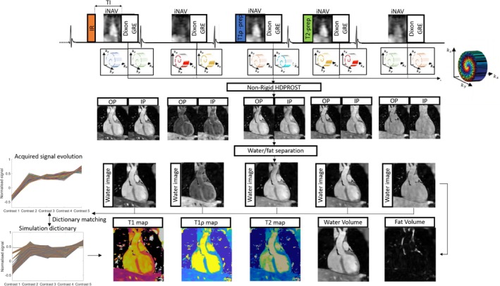 FIGURE 1
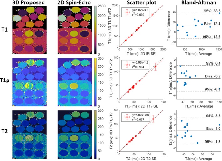 FIGURE 2
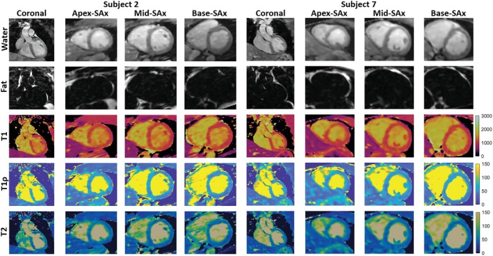 FIGURE 3
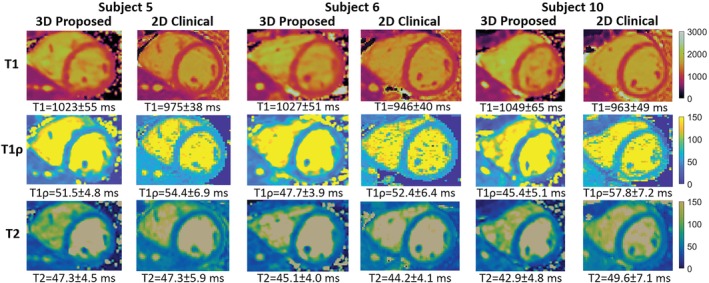 FIGURE 4
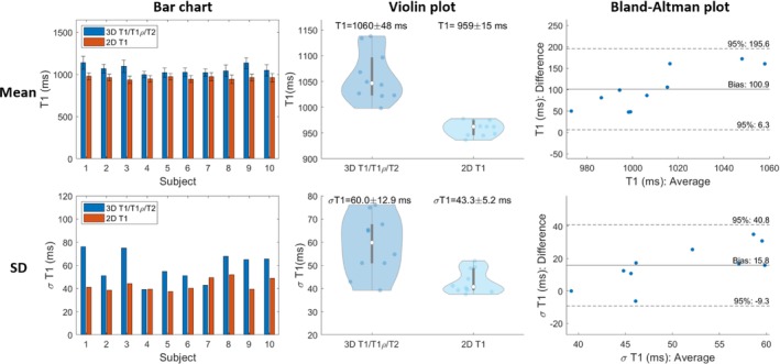 FIGURE 5
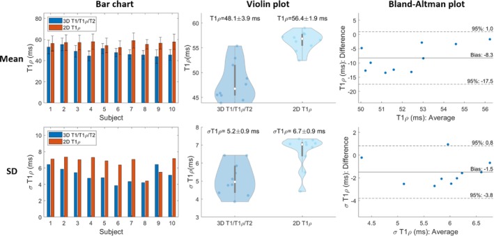 FIGURE 6
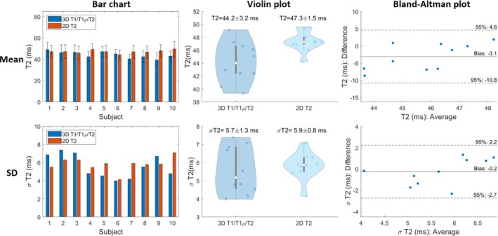 FIGURE 7
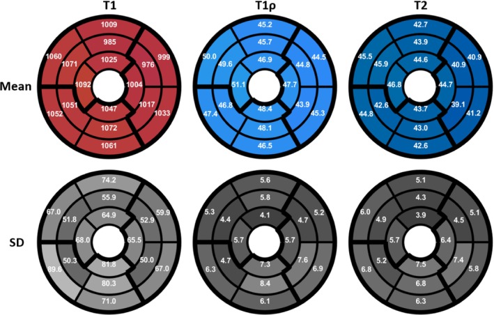 FIGURE 8
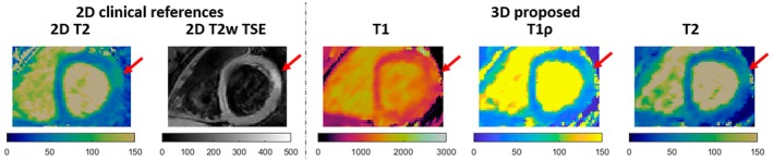 FIGURE 9
- —BHF: British Heart Foundation
- —British Heart Foundation 10.13039/501100000274
- —Millennium Institute for Intelligent Healthcare Engineering
- —Department of Health through the National Institute for Health Research (NIHR) comprehensive Biomedical Research Centre award 10.13039/501100000272
- —Engineering and Physical Sciences Research Council 10.13039/501100000266
- —IMPACT, Center of Interventional Medicine for Precision and Advanced Cellular Therapy
- —NIHR Cardiovascular MedTech Co‐operative
- —Fondo Nacional de Desarrollo Científico y Tecnológico 10.13039/501100002850
- —Institute for Advanced Study, Technische Universität München 10.13039/501100015072
- —Wellcome EPSRC Centre for Medical Engineering 10.13039/501100023312
Peer Reviews
No public reviews on file for this paper yet. If you reviewed it on a platform where reviews are public (OpenReview, ICLR, NeurIPS, ICML), you can paste yours below so the community can read it here.
Videos
No videos yet. Explain this paper in a talk, walkthrough, or lecture? Add one.
Taxonomy
TopicsCardiac Imaging and Diagnostics · Advanced MRI Techniques and Applications · Medical Imaging Techniques and Applications
INTRODUCTION
1
The use of gadolinium‐based contrast agents is clinically accepted for the detection of myocardial scar.1 However, in patients with renal dysfunction or contrast agent allergy, a non‐contrast‐enhanced approach would be of great value. Native T1, T1ρ, and T2 myocardial mapping have shown promising results in noninvasive detection of a range of different cardiomyopathies. This includes assessment of myocardial infarction and focal and diffuse fibrosis for T1,2, 3, 4, 5, 6 chronic myocardial infarction and fibrosis for T1ρ,7, 8, 9, 10 and assessment of inflammation and edema using T2,11, 12 thus helping to distinguish between acute and chronic infarction and providing complementary information for diagnosis. Furthermore, characterization of fibrofatty infiltration of the myocardium has been shown to be clinically relevant.13, 14
Myocardial maps are commonly acquired clinically through single‐parameter 2D mapping sequences, including MOLLI15 and SASHA16 for T1, and T2‐prep bSSFP17 for T2. These are usually acquired under a breath‐hold per short‐axis slice, yielding limited heart coverage and low spatial resolution. Also, additional heartbeats (HBs) are required to ensure magnetization recovery between preparation pulses. T1ρ mapping is less common clinically, but 2D breath‐hold sequences have recently been proposed.18, 19 However, these suffer from the same problems as previously mentioned for 2D mapping.
3D free‐breathing, single‐parameter mapping techniques have been proposed to remove the requirement of breath‐holds and increase heart coverage and spatial resolution. These include respiratory‐gated 3D mapping,20, 21 and respiratory motion‐compensated 3D mapping22, 23, 24 using 2D image navigators (iNAVs) and translational respiratory motion correction, leading to 100% respiratory scan efficiency and predictable scan time. However, these do not account for non‐rigid deformation of the heart through the respiratory cycle, but non‐rigid motion‐compensated reconstruction can be achieved through iNAV‐based translation motion estimation in concert with respiratory binning.25, 26, 27
Multi‐parametric mapping sequences, where several parameters are quantified in a single scan, may improve accuracy and protocol efficiency, simplify segmentation and analysis, and avoid misregistration over sequentially acquired sequences.28 For 2D multi‐parametric mapping, the most common parameters mapped are T1 and T2,29, 30, 31 but T1ρ has more recently been proposed in 2D joint T1/T1ρ mapping at 3T,32 2D T1/T2/T1ρ Magnetic Resonance Fingerprinting (MRF) at 1.5T,33 and 2D multi‐parametric T1/T2/T1ρ mapping at 3T.34 Fat quantification has been additionally incorporated in 2D T1/T2 MRF.35, 36 For 3D joint mapping, 3D joint T1/T2 mapping sequences that acquire data in the steady state have been proposed,37, 38 and a 3D joint T1/T2 mapping technique has recently been proposed that aims to provide co‐registered 3D T1 and T2 maps and water‐fat volumes with isotropic spatial resolution at 1.5T.28 A 3D joint T1/T1ρ mapping technique has also been proposed at 3T.39
The aim of this work was to develop a novel, free‐breathing, 3D whole‐heart joint T1/T1ρ/T2 mapping sequence with Dixon encoding to provide co‐registered 3D T1, T1ρ, and T2 maps and water‐fat volumes with isotropic spatial resolution in a single ≈7 min scan for comprehensive contrast‐agent‐free myocardial tissue characterization and simultaneous evaluation of the cardiac and coronary anatomy. A complementary co‐registered T2‐prepared bright‐blood water volume is obtained for whole‐heart anatomy visualization.
METHODS
2
Pulse sequence
2.1
The proposed ECG‐triggered 3D joint T1/T1ρ/T2 research sequence (Figure 1) consisted of a repeating set of preparation modules defined over 5 HBs: a 180° adiabatic IR pulse, no preparation, T1ρ preparation, T2 preparation, and no preparation. For T1ρ preparation, four spin‐locking pulses with alternating phases and two rectangular refocusing pulses with opposite phases were deployed to make T1ρ preparation more robust to B0 and B1 inhomogeneities.40, 41 A spin‐lock duration (TSL) =40ms and spin‐lock amplitude (SLA) =400Hz were used. For T2 preparation, two adiabatic refocusing pulses were deployed to make preparation more robust to B0 and B1 inhomogeneities42 with duration =40ms. The 5th idle HB is to compensate for T1 recovery for the next shot of the IR preparation and provide greater T1 sensitivity for longer T1 or heart‐rates (HRs). Five interleaved volumes were acquired with a 2‐point bipolar Dixon RF‐spoiled gradient recalled echo (GRE) readout with a variable‐density 3D Cartesian trajectory with spiral profile order (VD‐CASPR).43 A golden angle step within and across contrasts was used to ensure incoherent undersampling artifacts both within and across contrasts, with an acceleration factor = 6 per contrast chosen. 2D iNAVs44 were acquired prior to each 3D acquisition to enable beat‐to‐beat respiratory motion estimation and correction.
3D joint T1/T1ρ/T2 mapping and water/fat imaging sequence schematic diagram. Volume 1: IR (TI=250ms), Volume 2: no‐preparation, Volume 3: T1ρ‐preparation (spin‐lock duration =40ms and spin‐lock amplitude =400Hz), Volume 4: T2‐preparation (duration =40ms), Volume 5: no preparation. Non‐rigid motion correction with patch‐based regularization is used to reconstruct 3D IP/OP HB images; water and fat images are generated from IP/OP images through a fat‐water separation algorithm, and T1/T1ρ/T2 maps are estimated from water images by dictionary matching via a Bloch simulation of the proposed 3D sequence.
Dictionary generation and simulations
2.1.1
Numerical simulations of the proposed sequence were performed to generate signal dictionaries, as well as to test the accuracy and precision of the sequence (Supporting Information, Figure S1). A 1D Bloch equation simulation of the longitudinal magnetization, assuming perfect spoiling, was implemented in MATLAB (The MathWorks Inc., Natick, MA, USA) to generate a signal at each TR. The simulation consisted of 3 sets of 5 HBs, with the first 2 sets simulated to reach the steady‐state magnetization. The signal from the last set of 5 HBs was averaged over the first 30% of imaging readout (since data was acquired with centric k‐space reordering) to yield a dictionary with 5 points. Each signal evolution in the dictionary (corresponding to a unique parameter combination) was normalized. For in‐vivo data, subject‐specific dictionaries were generated using the mean RR interval and acquisition window. The dictionary used the following parameter combinations ([start:step:end]): T1=[50:50:600,600:15:1800,1800:50:2200,2200:100:3000]ms, T1ρ=[5:5:20,20:1.5:80,80:4:100,100:10:300,300:100:600]ms, T2=[5:5:20,20:1.5:80,80:4:100,100:10:300,300:100:600]ms, constrained such that T2≤T1ρ and T1ρ≤T1.
Image reconstruction
2.2
Motion correction
2.2.1
2D iNAVs were used to generate a low‐resolution 2D image in coronal orientation at each HB. Beat‐to‐beat translational Right‐Left (RL)/Foot‐Head (FH) respiratory motion fields were estimated from the iNAVs via normalized cross‐correlation. The estimated FH translational motion field was used to assign the acquired k‐space data for each contrast into a set of B=4 respiratory bins, and intra‐bin 2D translational motion (RL and FH) correction was performed by correcting the k‐space data for each bin to the same respiratory position (taken here as the bin centre).25 For non‐rigid motion estimation, binned images were reconstructed with iterative SENSE with soft‐binning25 using the respiratory binned k‐space data from 4th contrast, 1st echo. Non‐rigid registration using free‐form deformation45 was deployed on binned images, using end expiration bin as reference,46 yielding motion fields {Ub}b=1B. These were used to build the following motion‐correction encoding operator, E(c),
where Ab(c) is the binned sampling mask for bin b=1,…,B and contrast c=1,…,C, ℱ is the Fourier Transform, and S the coil sensitivities.47 Here, C=10 corresponds to the out‐of‐phase (OP) and in‐phase (IP) echoes for all 5 interleaved contrast acquisitions.
Patch‐based, low‐rank reconstruction
2.2.2
The 10 3D image contrasts were reconstructed using non‐rigid motion correction with patch‐based multi‐dimensional low‐rank regularization (HD‐PROST).27, 48 Image reconstruction was posed as minimisation of the following Lagrangian
where X are the contrast images, E = (E(1),…,E(c)) is the multi‐contrast encoding operator, K is the multi‐coil multi‐contrast translational motion‐corrected k‐space data, and Pv(X) is the patch selection operator for voxel v, Tv is a tensor of patches similar to the patch at the vth voxel, Y is a Lagrange multiplier, μ, λ are regularization parameters, and ||·||∗/F are nuclear/Frobenius norms. The Alternating Direction Method of Multipliers (ADMM) method49 was used to solve this problem. For each outer iteration of ADMM, the minimization is performed by the sequential solution of the following 3 sub‐problems: (i) regularized MR reconstruction (minimization of (2) wrt X, with T,Y fixed) solved using iterative SENSE (5 iterations); (ii) denoising (minimization of (2) wrt T, with X,Y fixed) solved using higher‐order singular value decomposition and truncation, and (iii) Lagrange multiplier update of T. These sub‐problems are repeated over 5 outer ADMM iterations and regularization parameters, λ=0.04 and μ=0.1 are selected. For the patch‐based denoising step 2, other parameters selected include a voxel search window =20×20×20, a voxel patch size =5×5×5, a number of selected similar patches =20, and a voxel patch offset = 4 when searching for similar patches (see27, 50 for definitions and further details).
Water/fat separation
2.2.3
Water and fat images for all 5 interleaved contrast acquisitions were subsequently estimated from the corresponding reconstructed IP/OP images via background phase correction to eliminate errors due to B0 inhomogeneity using the B0‐NICE method.51
Mapping
2.2.4
For the generation of signal dictionaries, a simulation of the sequence was implemented in MATLAB as outlined in section 2.1.1. The signal polarity was estimated through background phase‐removal using the 4th contrast IP echo image,52 and the polarity‐restored water images were normalized across contrasts for each image voxel. Matching was performed voxel‐wise by selecting the parameter corresponding to the maximum inner‐product of the normalised measured signal with the dictionary.
Experiments
2.3
The proposed 3D joint T1/T1ρ/T2 sequence was tested in phantoms, healthy subjects, and patients. Data was acquired on a 1.5T MR scanner (MAGNETOM Aera, Siemens Healthineers AG, Erlangen, Germany) with an 18‐channel chest array and a 32‐channel spine array. Written informed consent was obtained from all participants before undergoing the MR scan, and the study was approved by the institutional review board.
Phantoms
2.3.1
Data was acquired in a T1‐MES phantom53 and an in‐house phantom with vials of variable agar/NiCl2 concentration.33 The mapping values obtained with the proposed approach were compared with 2D IR‐prep Spin‐Echo (IR SE), 2D T1ρ‐prep SE, and 2D T2 SE measurements for both accuracy and precision.
The proposed 3D joint T1/T1ρ/T2 mapping was acquired with 2‐point bipolar Dixon GRE read‐out (TE1/TE2/TR=2.38/4.76/6.71ms, flip angle (FA) =8°, bandwidth (BW) =453Hz/pixel), iNAV (14(×2)‐echoes, FA=3°), TI=250ms, VD‐CASPR acceleration =×6/contrast with centric k‐space reordering, FOV=320×320×20mm3, resolution =2mm isotropic. 16 segments were acquired per HB, corresponding to an acquisition window =107ms.
For 2D IR SE, imaging parameters included TE/TR=11/10000ms, FA=90°, resolution =2×2mm2, slice‐thickness =8mm, BW=130Hz/pixel. 9 IR‐preps with TIs=[50,350,650,950,1250,1550,1850,2150,2450]ms were used. A 2‐parameter fit, (T1,M0), to the following signal equation S(T1,M0,TI,TR)=M0(1−2exp(−TI/T1)+exp(−TR/T1)) was used, solved using the Levenberg‐Marquardt algorithm.
For 2D T1ρ‐prep SE, imaging parameters included TE/TR=12/5000ms, FA=90°, resolution =2×2mm2, slice‐thickness =8mm, BW=130Hz/pixel. 8 T1ρ‐preps with TSL =[2,14,26,38,50,62,74,86]ms and SLA =400Hz were used. A 1‐parameter fit T1ρ to the log of the following signal equation, S(T1ρ,M0,TSL)=M0exp(−TSL/T1ρ), was obtained through linear least‐squares fitting.
For 2D T2 SE, imaging parameters included TR=10000ms, FA=90°, resolution =2×2mm2, slice‐thickness =8mm, BW=130Hz/pixel. 8 images with TEs=[12,27,42,57,72,87,102,117]ms were acquired. A 1‐parameter fit T2 to the log of the following signal equation, S(T2,M0,TE)=M0exp(−TE/T2), was obtained through linear least‐squares fitting.
Healthy subjects
2.3.2
Data was acquired in 10 healthy subjects. The accuracy and precision of values from the proposed mapping sequence were compared to 2D MOLLI,15 2D T1ρ‐prep bSSFP,24 and 2D T2‐prep bSSFP17 mapping sequences at mid‐ventricular short‐axis (SAx) slice. Two‐tailed Student's t‐tests (p<0.05) were used to analyze differences in mean/SD T1/T1ρ/T2 values.
For the proposed 3D joint T1/T1ρ/T2 mapping, a subject‐specific slice selection covering the heart (FOV=320×320×96−120mm3) was planned following acquisition of a cardiac localiser. Imaging was performed at mid‐diastole with a trigger delay and acquisition window informed through acquisition of a free‐breathing 4‐chamber CINE. The acquisition window was 124±16ms. The remaining imaging parameters matched those used for phantoms. The total acquisition time was 7.3±0.8 mins.
For 2D MOLLI, the MOLLI 5(3)3 sequence15 was deployed with bSSFP readout with TE/TR=1.12/2.8ms, FA=35°, resolution =1.6×1.6mm2, slice‐thickness =8mm, and BW=1085Hz/pixel. The T1 weighted images and maps were obtained inline on the scanner.
For 2D T1ρ, an ECG‐triggered 2D T1ρ‐prepared bSSFP reference sequence24 was acquired during a breath‐hold at mid‐diastole and consists of the acquisition of 5 T1ρ‐prepared images with TSL =[1,10,20,35,50]ms and SLA =400Hz. A saturation (SAT) pulse was deployed at each HB with a constant delay prior to T1ρ‐preparation. A bSSFP readout was used with TE/TR=1.2/3.3ms (partial Fourier in readout direction), FA=50°, and parallel imaging using GRAPPA (acceleration factor ×2), FOV=300×300mm2, resolution =2×2mm2, slice‐thickness =8mm. A fixed 170ms acquisition window was used, corresponding to 3 HBs/contrast and a scan time of 15 HBs per short‐axis slice. Mono‐exponential fitting was used to generate T1ρ maps from the reconstructed T1ρ‐weighted images, working through image voxel by voxel.
For 2D T2, the 2D T2‐prepared bSSFP sequence17 was deployed with 3 T2‐prepared images acquired (T2‐prep durations =[0,25,55]ms) and 3 recovery beats. A bSSFP readout with TE⁄TR=1.06⁄2.49ms, FA=70°, resolution =1.9×1.9mm2, slice‐thickness =8mm, BW=1185Hz/pixel, and linear k‐space reordering was used. The T2 weighted images and maps were obtained inline on the scanner.
Patients
2.3.3
The proposed 3D joint T1/T1ρ/T2, 2D MOLLI, 2D T1ρ‐prep bSSFP, and 2D T2‐prep bSSFP sequences were acquired in 1 patient with suspected cardiovascular disease. Acquisition parameters matched those used for healthy subjects. For the patient, T2‐weighted Turbo Spin Echo (T2w‐TSE)54 (1.5×1.5×8 mm3) was additionally acquired in several SAx views.
RESULTS
3
Phantoms
3.1
For phantom results, we first show a comparison of the proposed 3D T1/T1ρ/T2 mapping sequence and 2D IR SE, 2D T1ρ‐prep SE, and 2D T2 SE references with a simulated HR = 60 bpm in Figure 2. High linear correlations of y=1.02x−3.8 (r2=0.999), y=0.96x−1.3 (r2=0.994), and y=1.00x+0.9 (r2=0.997) were observed when comparing the 3D joint T1/T1ρ/T2 sequence to 2D IR SE, 2D T1ρ‐prep SE, and 2D T2 SE, respectively. Small biases of +12ms, −3.2ms and +1.0ms for proposed T1, T1ρ, and T2 were observed, respectively. Vials with T1≥1500ms, T1ρ≥150ms, and T2≥150ms were rejected prior to fitting to focus on the typical myocardial tissue value range. Generally, vials with large T1, T1ρ or T2 were less accurate and precise, since the sequence is designed for values within the myocardium. In particular, for T1ρ and T2, the proposed sequence only uses a single T1ρ‐prep and T2‐prep, each with a 40 ms duration, and, for T1, there are only 5 HBs between IR pulses. Experiments were also performed to compare the proposed mapping sequence with 2D SE references over a range of simulated HRs (Supporting Information, Figure S2).
Left: Comparison of proposed 3D T1/T1ρ/T2 mapping to 2D IR SE, 2D T1ρ‐prep SE, and 2D T2 SE (simulated heart‐rate (HR)=60 bpm). The top 10 vials are from the in‐house phantom, and the bottom 9 vials are from the T1‐MES phantom. Middle: Scatter plot comparison of proposed 3D T1/T1ρ/T2 to 2D SE mapping references. The black and red lines are identity lines and linear fits, respectively. Right: Bland‐Altman plot comparison of proposed 3D T1/T1ρ/T2 to 2D SE mapping references.
Healthy subjects
3.2
Figure 3 shows different views of the 3D volume of Water (4th contrast), Fat (4th contrast), T1, T1ρ, and T2 maps in 2 representative healthy subjects. Good quality water and fat volumes and maps are observed, with clear definition of the myocardium in both subjects. Water and fat contrast images for each of the 5 contrast interleaved acquisitions for a representative subject are shown in Supporting Information, Figure S3. A 16‐segment AHA model55 was calculated on the reformatted SAx slices for each of the reconstructed 3D T1, T1ρ, and T2 maps for all healthy subjects. Mean and Standard Deviation (SD) were calculated for each segment of the AHA model. Figure 4 illustrates mid‐ventricular SAx views of the proposed 3D T1/T1ρ/T2 maps, 2D MOLLI, 2D T1ρ‐prep bSSFP, and 2D T2‐prep bSSFP for 3 representative healthy subjects, and good qualitative agreement is observed between the 3D proposed and 2D reference maps. SAx views of the 3D proposed maps extending from apex to base, high‐resolution Bull's eye plots, and histograms of measured left‐ventricle mapping values for a representative healthy subject are demonstrated for T1, T1ρ, and T2 in Supporting Information Figure S4, S5, and S6 respectively.
Water (4th HB), Fat (4th HB), T1, T1ρ, and T2 mappings from the proposed 3D joint T1/T1ρ/T2 mapping sequence with Dixon encoding showing coronal, apex‐, mid‐, and base‐ventricular short‐axis (SAx) views through the 3D reconstruction in 2 healthy subjects.
Comparison of 3D T1/T1ρ/T2 to 2D references at mid‐ventricular short‐axis (SAx) for 3 representative healthy subjects. The mean and standard deviation of mid‐ventricular SAx septal myocardium values are displayed.
For all subjects, the myocardium of a mid‐SAx slice was segmented for the proposed 3D T1/T1ρ/T2 mapping, 2D MOLLI, 2D T1ρ‐prep bSSFP, and 2D T2‐prep bSSFP. Figures 5, 6, 7 illustrate a comparison of mid‐SAx septal myocardium values between the proposed and reference sequences across all healthy subjects for T1, T1ρ, and T2, respectively. For T1, mean septal values for the proposed 3D T1/T1ρ/T2 sequence (1060±48ms) were significantly higher (p<0.0001) than for 2D MOLLI (959±15ms). For T1, SD for the proposed sequence (60±13ms) was significantly higher (p=0.004) than 2D MOLLI (43±5ms). For T1ρ, the mean septal value across subjects for the proposed 3D T1/T1ρ/T2 sequence (48.1±3.9ms) was significantly smaller (p<0.0001) than 2D T1ρ‐prep bSSFP (56.4±1.9ms). For T1ρ, SD for the proposed sequence (5.2±0.9ms) was significantly smaller (p=0.002) than 2D T1ρ‐prep bSSFP (6.7±0.9ms). For T2, the mean septal value across subjects for the proposed 3D T1/T1ρ/T2 sequence (44.2±3.2ms) was significantly smaller (p=0.02) than 2D T2‐prep bSSFP (47.3±1.5ms). For T2, SD for the proposed sequence (5.7±1.3ms) was slightly smaller than 2D T2‐prep bSSFP (5.9±0.8ms), but not significantly.
Comparison of mid‐ventricular short‐axis septal myocardium values for proposed T1 and 2D MOLLI across healthy subjects. Top/Bottom figures are the Mean/Standard Deviation (SD) of myocardial values Left to Right are Bar chart, Scatter, Violin and Bland‐Altman plots.
Comparison of mid‐ventricular short‐axis septal myocardium values for proposed T1ρ and 2D T1ρ‐prep bSSFP across healthy subjects. Top/Bottom figures are the Mean/Standard Deviation (SD) of myocardial values. Left to Right are Bar chart, Violin, and Bland‐Altman plots.
Comparison of mid‐ventricular short‐axis septal myocardium values for proposed T2 and 2D T2‐prep bSSFP across healthy subjects. Top/Bottom figures are the Mean/Standard Deviation (SD) of myocardial values. Left to Right are Bar chart, Violin, and Bland‐Altman plots.
Bull's eye plots of mean/SD for T1/T1ρ/T2 averaged across all healthy subjects are shown for proposed 3D joint T1/T1ρ /T2 mapping in Figure 8, demonstrating uniform T1, T1ρ, and T2 values over the 16 AHA segments. Violin plots of mean and SD for T1, T1ρ, and T2 for each AHA segment across all subjects are shown in Supporting Information Figure S7. Left‐ventricle myocardium values were computed for the proposed sequence, averaged across all healthy subjects. For T1 Mean/SD = 1034±19ms/83.0±15.8ms, for T1ρ Mean/SD = 47.0±1.6ms/7.2±1.6ms, and for T2 Mean/SD = 43.3±1.6ms/7.0±1.4ms. Mean/SD T1, T1ρ, and T2 values across all healthy subjects for different regions of the heart are tabulated in Supporting Information Table S1.
Bull's eye plots of Mean and Standard Deviation (SD) for T1, T1ρ, and T2 (ms) for proposed 3D joint T1/T1ρ/T2 mapping averaged across all 10 healthy subjects.
We compare values between mid, base, and apex segments. Mean T1 in base, mid, and apex segments was calculated to be 1036±24ms, 1029±24ms, and 1042±25ms. SD T1 in base, mid, and apex segments was calculated to be 72±14ms, 58±13ms, and 70±16ms. There were no significant differences for mean or SD between these segments, apart from SD T1 base which was significantly higher than mid (p=0.03). Mean T1ρ in base, mid, and apex segments was calculated to be 46.5±2.0ms, 46.5±2.3ms, and 48.5±1.8ms. SD T1ρ in base, mid and apex segments was calculated to be 5.9±1.2ms, 6.1±1.5ms, and 5.8±1.0ms. There were no significant differences for mean or SD between these segments, apart from mean T1ρ apex was significantly higher than mid (p=0.04) and base (p=0.03). Mean T2 in base, mid and apex segments was calculated to be 42.9±1.5ms, 42.6±1.8ms, and 45.0±2.3ms. SD T2 in base, mid and apex segments was calculated to be 5.9±1.3ms, 5.6±1.8ms, and 6.0±1.4ms. There was no significant differences for mean or SD between these segments, apart from mean T2 for apex, which was significantly higher than mid (p=0.02) and base (p=0.03).
We now compare values between anterior, inferior, septal, and lateral segments. Mean T1 in anterior, inferior, septal, and lateral segments was calculated to be 1007±23ms, 1060±39ms, 1065±37ms, and 1005±21ms. SD T1 in anterior, inferior, septal, and lateral segments was calculated to be 65±14ms, 78±18ms, 67±11ms, and 60±16ms. Comparing septal and lateral segments, and anterior and inferior segments, mean T1 septal was significantly larger (p<0.001) than lateral T1, and mean T1 inferior was significantly larger (p=0.002) than anterior T1. Mean T1ρ in anterior, inferior, septal, and lateral segments was calculated to be 45.9±3.3ms, 47.7±3.6ms, 49.0±2.6ms, and 45.2±2.0ms. SD T1ρ in anterior, inferior, septal, and lateral segments was calculated to be 5.2±1.6ms, 7.3±2.0ms, 5.4±0.8ms, and 6.1±1.6ms. Comparing septal and lateral segments, and anterior and inferior segments, the mean T1ρ septal was significantly larger (p=0.002) than lateral T1ρ, and SD T1ρ inferior was significantly larger (p=0.02) than anterior T1ρ. Mean T2 in anterior, inferior, septal, and lateral segments was calculated to be 43.8±3.0ms, 43.1±3.4ms, 45.1±2.2ms, and 41.4±1.4ms. SD T2 in anterior, inferior, septal, and lateral segments was calculated to be 4.5±1.0ms, 6.9±2.3ms, 5.7±1.2ms, and 5.9±1.6ms. Comparing septal and lateral segments and anterior and inferior segments, mean T2 septal was significantly larger (p<0.001) than lateral T2, and SD T2 inferior was significantly larger (p=0.02) than anterior T2.
Patients
3.3
Results from a patient with active myocarditis involving the left ventricle lateral wall are shown in Figure 9. Increased myocardial signal intensity in the basal‐anterolateral segments is observed in the clinical reference 2D T2 maps and 2D T2w‐TSE images in the first 2 columns. The proposed 3D T1/T1ρ/T2 mapping indicates elevated T2 values (as well as T1ρ and T1 values) in the corresponding region. Remote/basal‐anterolateral T2 values were 45±2ms/78±4ms and 42±5ms/66±3ms for 2D reference and 3D proposed, respectively. Remote/basal‐anterolateral T1 and T1ρ values for the proposed sequence were estimated to be: T1=1081±55ms/1319±69ms and T1ρ=46±2ms/71±3ms respectively.
Comparison of 3D T1/T1ρ/T2 with 2D LGE at a basal SAx slice for a patient with active myocarditis. Increased myocardial signal intensity can be observed in both the clinical 2D T2 map and 2D T2‐weighted Turbo Spin Echo (T2w‐TSE) images. The proposed sequence indicates elevated T2 (as well as T1ρ and T1) in the corresponding region.
DISCUSSION
4
A novel free‐breathing, 3D joint T1/T1ρ/T2 mapping sequence with Dixon encoding has been proposed to provide co‐registered 3D T1, T1ρ, and T2 maps and water‐fat volumes with isotropic spatial resolution in a single ≈7 min scan for comprehensive contrast‐agent‐free myocardial tissue characterization and simultaneous evaluation of the whole‐heart anatomy. The proposed sequence is an extension of the sequence proposed in28 but with additional T1ρ magnetization preparation, since T1ρ mapping has shown to be more sensitive to the detection of fibrotic tissue. The proposed sequence also uses a 2nd angle increment across contrasts to increase the incoherence of undersampling artifacts in order to improve the performance of the patch‐based low‐rank regularization algorithm and enable higher undersampling factors. Additionally, the proposed framework has been extended to incorporate non‐rigid respiratory motion correction to the reconstructed volumes and subsequent maps.
The proposed free‐breathing mapping sequence provides 3D whole‐heart co‐registered water and fat volumes and T1, T1ρ, and T2 maps in a clinically feasible time, addressing some of the previously mentioned limitations of 2D clinical mapping sequences acquired during a typical CMR examination. In phantoms, the proposed technique demonstrated good correlation with reference T1/T1ρ/T2 SE values with a high coefficient of determination after a linear fit. The proposed sequence was compared to in‐vivo 2D MOLLI, 2D T1ρ‐prep bSSFP, and 2D T2‐prep bSSFP mapping sequences in 10 healthy subjects. For T1, statistically significant larger mean and SD values were observed with proposed mapping than 2D MOLLI. The bias in mean T1 could be explained by the known underestimation of T1 by MOLLI.56 For T1ρ and T2, statistically significant shorter mean values were observed with proposed mapping compared to reference 2D T1ρ‐prep bSSFP and 2D T2‐prep bSSFP, respectively, but the latter methods could be overestimating due to the unaccounted effect of imaging pulses during bSSFP readout.57 A whole‐heart analysis over all healthy subjects demonstrated some differences when comparing mapping values in basal, mid, and apical segments, with mean T1ρ and T2 for apical segments being significantly shorter than mid and basal segments (p=0.02−0.04). Comparing anterior and inferior segments, mean T1 inferior were significantly larger than anterior (p=0.002), and SD T1ρ and T2 inferior was significantly larger than anterior (p=0.02). Comparing septal and lateral segments, mapping values in lateral segments were significantly shorter than septal segments for T1 (p<0.001), T1ρ (p=0.002), and T2 (p<0.001). Similar underestimation has been reported previously22, 28 and may be due to greater susceptibility artifacts at the lung‐myocardium interface and reduced coil sensitivity in lateral segments.58 The proposed sequence was acquired in 1 patient with active myocarditis and demonstrated good correlation with clinical 2D T2‐prep bSSFP and 2D T2w‐TSE.
This study has some limitations. First, the sequence could be sensitive to arrhythmias, since the assumed steady‐state signal would be affected by arrhythmic beats, potentially causing a loss of accuracy and precision in mapping values. The integration of prospective and retrospective arrhythmia rejection will be considered in future work. Second, only a small number of healthy subjects and patients were scanned, but further work will include acquisition of a larger cohort of healthy subjects and patients with different cardiovascular diseases to assess the suitability of the proposed mapping sequence for myocardial tissue characterization. Third, coils were manually selected in this work, but in future automatic coil selection techniques will be considered.59 Fourth, the sequence has potentially reduced T2 and T1ρ sensitivity since there is only a single T2‐prep and T1ρ‐prep pulse per repetition, potentially limiting clinical usage of the sequence. Further work will include the use of an additional T1ρ‐prep and T2‐prep module to increase the encoding strength and improve sensitivity to T1ρ and T2, at the expense of a longer 7 HB preparation sequence repetition. To offset the increase in scan time that would result, a further increase in VD‐CASPR acceleration or reduction of FOV (e.g., changing orientation to 3D short‐axis) will be explored. Additionally, an increase in spatial resolution would be considered to improve image quality. Super‐resolution techniques based on an end‐to‐end deep learning non‐rigid motion‐corrected reconstruction network will be considered to maintain a clinically feasible scan time.60, 61, 62, 63
Finally, an SLA =400 Hz was used in this study, but increasing SLA up to ≈1 kHz could better match physical processes of macromolecular‐water interactions in infarcted regions of the myocardium and thus increase the sensitivity of the proposed mapping to detect fibrosis. The maximal SLA is limited both by the maximum power of the RF amplifier as well as SAR constraints. Hence, it may be desirable to perform T1ρ‐mapping at lower‐field, where SAR limitations (SAR∝|B0|2) are decreased, and a future study will aim to acquire the proposed mapping sequence at lower B0 field strengths.
CONCLUSIONS
5
A novel free‐breathing, 3D joint T1/T1ρ/T2 mapping sequence with Dixon encoding was proposed to provide co‐registered 3D T1, T1ρ and T2 maps and water‐fat volumes with isotropic spatial resolution in a single ≈ 7 min scan for comprehensive contrast‐agent free myocardial tissue characterization and simultaneous evaluation of the whole‐heart anatomy. 3D joint T1/T1ρ/T2 mapping and fat imaging results demonstrate good quantitative agreement when comparing to 2D T1, T1ρ, and T2 references in phantoms and 10 healthy subjects. Data was acquired in 1 patient with active myocarditis, and promising results were obtained when comparing it to conventional 2D T2w‐TSE.
CONFLICT OF INTEREST STATEMENT
K. P. Kunze is an employee of Siemens Healthcare Limited.
Supporting information
Data S1. Supporting Information. Figure S1. Simulation of sequence precision and accuracy, with N _ n _ = 1000 noise realisations with SNR = 70 dB. Left to Right figures indicates (Bias) and Coefficient of Variation (CoV) for fixed T 1 = 1100 ms, fixed T 1ρ = 56 ms, and fixed T 2 = 44 ms. Top to Bottom are T 1/T 1ρ/T 2 values. Figure S2. Comparison of proposed 3D T 1/T 1ρ/T 2 values to 2D T 1 SE, 2D T 1ρ SE, and 2D T 2 SE in T 1‐MES and in‐house phantoms as function of simulated HR = [60, 80, 100, 120] bpm. Vials with T 1 ≥ 1500 ms, T 1ρ ≥ 150 ms, T 2 ≥ 150 ms were rejected to focus on typical myocardial tissue values. Left: Scatter plots including the coefficient of determination from a linear fit, and the black dashed lines are the identity line. Right: Bar charts of Mean and Coefficient of Variation (CoV) estimation for each vial for proposed 3D T 1/T 1ρ/T 2 mapping and 2D SE references. Good agreement is observed between 3D proposed and 2D SE references with an r ^2^ > 0.993 over all simulated HR and T 1/T 1ρ/T 2. Figure S3. 3D Water and Fat images for each volume from the proposed 3D joint T 1/T 1ρ/T 2 mapping sequence with Dixon encoding in mid‐coronal view for one representative healthy subject. Figure S4. Whole‐heart analysis of T 1 for one representative healthy subject (Subject 7): (A) T 1 maps in short‐axis view from apex to base, (B) high‐resolution Bull's eye plots of Mean (normalised to mean across whole left ventricle myocardium)/Coefficient of Variation (CoV) T 1 with the Mean(normalised)/CoV(%) of each AHA segment displayed, (C) histogram of T 1 values across the whole left‐ventricle with measured T 1 = 1039 ± 81 ms, CoV = 7.8%. Figure S5. Whole‐heart analysis of T 1ρ for one representative healthy subject (Subject 7): (A) T 1ρ maps in short‐axis view from apex to base, (B) high‐resolution Bull's eye plots of Mean (normalised to mean across whole left ventricle myocardium)/Coefficient of Variation (CoV) T 1ρ with the Mean(normalised)/CoV(%) of each AHA segment displayed, (C) histogram of T 1ρ values across the whole left‐ventricle with measured T 1ρ = 46.7 ± 6.7 ms, CoV = 14.4%. Figure S6. Whole‐heart analysis of T 2 for one representative healthy subject (Subject 7): (A) T 2 maps in short‐axis view from apex to base, (B) high‐resolution Bull's eye plots of Mean (normalised to mean across whole left ventricle myocardium)/Coefficient of Variation (CoV) T 2 with the Mean(normalised)/CoV(%) of each AHA segment displayed, (C) histogram of T 2 values across the whole left‐ventricle with measured T 2 = 42.5 ± 6.5 ms, CoV = 15.3%. Figure S7. Violin plots of Mean and Standard Deviation myocardium values for T 1/T 1ρ/T 2 across all healthy subjects over all 16 AHA segments. Ba = Basal, Mi = Mid, Ap = Apex, A = Anterior, I = Inferior, S = Septal, L = Lateral. Table S1. Mean/Standard Deviation (SD) myocardium T 1, T 1ρ and T 2 values of 10 healthy volunteers in different regions of the heart measured with the proposed 3D whole‐heart joint T 1/T 1ρ/T 2 mapping sequence.
The reference list from the paper itself. Each links out to its DOI / PubMed record.
- 1Kim RJ , Wu E , Rafael A , et al. The use of contrast‐enhanced magnetic resonance imaging to identify reversible myocardial dysfunction. N Engl J Med. 2000;343:1445‐1453.10.1056/NEJM 20001116343200311078769 · doi ↗ · pubmed ↗
- 2Haaf P , Pankaj G , Messroghli DR , Broadbent DA , Greenwood JP , Plein S . Cardiac T 1 mapping and extracellular volume (ECV) in clinical practice: a comprehensive review. J Cardiovasc Magn Reson. 2016;18:89.10.1186/s 12968-016-0308-4PMC 512925127899132 · doi ↗ · pubmed ↗
- 3Messroghli DR , Walters K , Plein S , et al. Myocardial T 1 mapping: application to patients with acute and chronic myocardial infarction. Magn Reson Med. 2007;58:34‐40.17659622 10.1002/mrm.21272 · doi ↗ · pubmed ↗
- 4Bull S , White SK , Piechnik SK , et al. Human non‐contrast T 1 values and correlation with histology in diffuse fibrosis. Heart. 2013;99:932‐937.23349348 10.1136/heartjnl-2012-303052 PMC 3686317 · doi ↗ · pubmed ↗
- 5Puntmann VO , Voigt T , Chen Z , et al. Native T 1 mapping in differentiation of normal myocardium from diffuse disease in hypertrophic and dilated cardiomyopathy. JACC Cardiovasc Imaging. 2013;6:475‐484.23498674 10.1016/j.jcmg.2012.08.019 · doi ↗ · pubmed ↗
- 6Moon JC , Messroghli DR , Kellman P , et al. Myocardial T 1 mapping and extracellular volume quantification: a Society for Cardiovascular Magnetic Resonance (SCMR) and CMR working Group of the European Society of cardiology consensus statement. J Cardiovasc Magn Reson. 2013;15:92.10.1186/1532-429X-15-92PMC 385445824124732 · doi ↗ · pubmed ↗
- 7Witschey WRT , Zsido GA , Koomalsingh K , et al. In‐vivo chronic myocardial infarction characterization by spin locked cardiovascular magnetic resonance. J Cardiovasc Magn Reson. 2012;14:37.22704222 10.1186/1532-429X-14-37PMC 3461454 · doi ↗ · pubmed ↗
- 8van Oorschot JWM , El Aidi H , Lorkeers SJ , et al. Endogenous assessment of chronic myocardial infarction with T(1ρ)‐mapping in patients. J Cardiovasc Magn Reson. 2014;16:104.10.1186/s 12968-014-0104-y PMC 427254225526973 · doi ↗ · pubmed ↗