Protocol for assessing distances in pathway space for classifier feature sets from machine learning methods
Bahar Tercan, Victor H. Apolonio, Vinicius S. Chagas, Christopher K. Wong, Jordan A. Lee, Christina Yau, Christopher C. Benz, Joshua M. Stuart, Brian J. Karlberg, Kyle Ellrott, Jasleen K. Grewal, Steven J.M. Jones, Theo A. Knijnenberg, Theo A. Knijnenberg, Mauro A.A. Castro

TL;DR
This paper introduces a protocol to assess biological relationships between gene sets identified by different machine learning methods using pathway space analysis.
Contribution
A novel protocol is introduced to evaluate the biological relevance of distinct gene sets in pathway space using the PathwaySpace R package.
Findings
The protocol enables testing if seemingly different gene sets are biologically related in pathway space.
Steps are provided for building a pathway space and calculating pathway distances between gene sets.
Density plots and pathway distance metrics help visualize and quantify relationships between gene sets.
Abstract
As genes tend to be co-regulated as gene modules, feature selection in machine learning (ML) on gene expression data can be challenged by the complexity of gene regulation. Here, we present a protocol for reconciling differences in classifier features identified using different ML approaches. We describe steps for loading the PathwaySpace R package, preparing input for analysis, and creating density plots of gene sets. We then detail procedures for testing whether apparently distinct feature sets are related in pathway space. For complete details on the use and execution of this protocol, please refer to Ellrott et al.1 •Protocol to test whether distinct gene sets reflect related biology•Steps for building a pathway space for graph- or network-based distance analysis•Instructions for calculating a pathway distance metric for any pair of gene sets•Guidance on exploring relationships…
Genes, proteins, chemicals, diseases, species, mutations and cell lines named across the full text — each resolved to its canonical identifier and authoritative record.
Click any figure to enlarge with its caption.
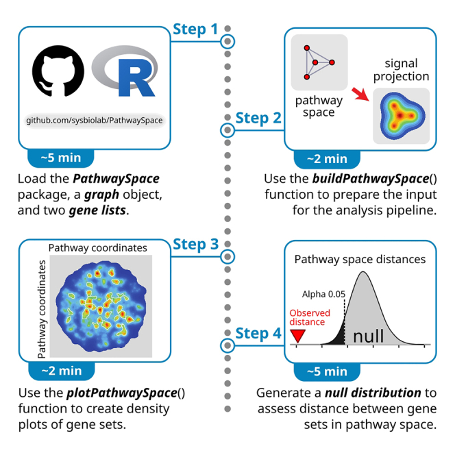 Figure 1
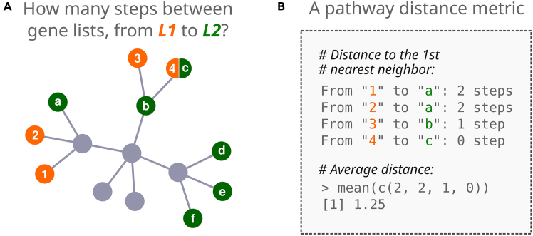 Figure 2
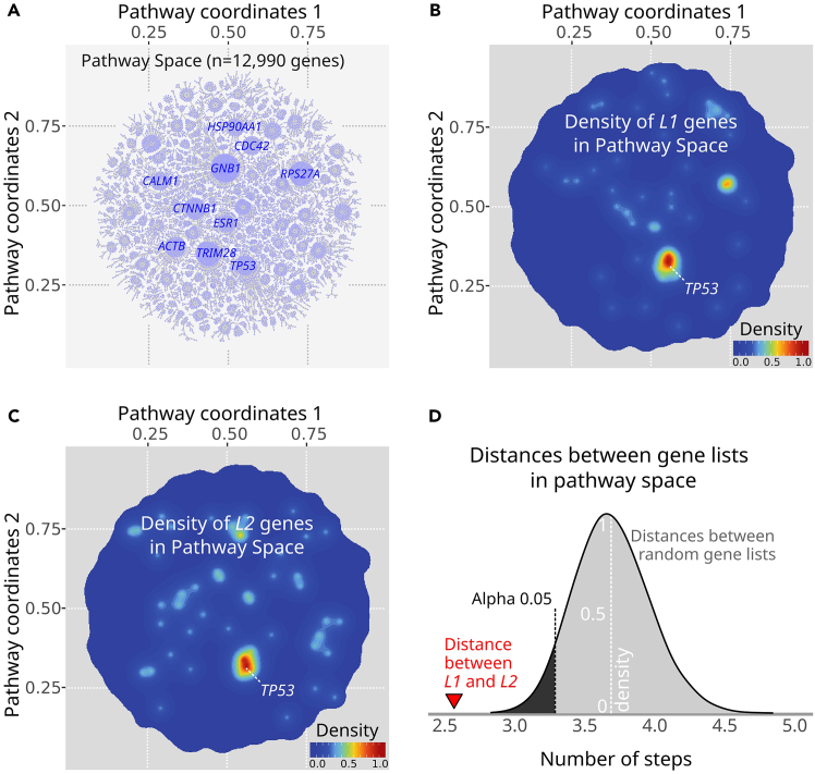 Figure 3
Peer Reviews
No public reviews on file for this paper yet. If you reviewed it on a platform where reviews are public (OpenReview, ICLR, NeurIPS, ICML), you can paste yours below so the community can read it here.
Videos
No videos yet. Explain this paper in a talk, walkthrough, or lecture? Add one.
Taxonomy
TopicsMachine Learning in Bioinformatics · Rough Sets and Fuzzy Logic · Bioinformatics and Genomic Networks
Before you begin
Overview
We generated a general method by which gene features that are identified through machine learning (ML) algorithms can classify non-TCGA tumors into TCGA subtypes.1 We found that ML algorithms often produced non-overlapping classifier feature sets that had similar accuracy profiles. We showed that distinct ML classifier features tended to reflect coregulated genes from the same pathways, and the pathways carry comparable biological information for subtype classification. Here, we present a protocol that allows comparing pathway distances between lists of genes. We describe steps involved in constructing a two-dimensional (2D) 'pathway space' in order to visualize and quantify the degree to which different gene sets are related. The R package PathwaySpace provides the data and source code required to execute all steps of this protocol.
The pathway distance problem
For this protocol, we implemented a new metric to statistically assess distances between vertices. As an example, we introduce this metric in Figure 1A, presenting both a schematic pathway space graph and two hypothetical gene lists, L1 and L2. We calculate a distance between these lists as the average path distance to first nearest neighbors (Figure 1B). In the protocol that follows, while there is minimal overlap between genes in L1 and L2, we test whether these two gene lists are positioned more closely to each other in pathway space than we would expect by chance.Figure 1. The pathway distance problem addressed by the PathwaySpace package(A) A schematic pathway space with 'toy' gene lists L1 and L2. The package addresses the question: “How many steps are required to 'walk' from L1 to L2?”.(B) The average path distance to the first nearest neighbors, between gene lists L1 and L2, is 1.25.
Computational requirement
Hardware: RAM >= 16 GB.
Software: R (>=4.4), RStudio and PathwaySpace.
Software installation
Timing: ∼30 min
In this step, we download and install R and RStudio, followed by the PathwaySpace package.
- 1.Download and install R and RStudio.
- a.To download R: https://cran.r-project.org/
- b.To download RStudio: https://rstudio.com/products/rstudio/
- 2.Download and install PathwaySpace in RStudio:
install.packages("PathwaySpace")Note: Additional R dependencies will be automatically downloaded during installation, including RGraphSpace, igraph, ggplot2, ggrepel, RANN, and scales packages.
Key resources table
REAGENT or RESOURCESOURCEIDENTIFIERDeposited dataPruned Pathway Commons v.12Ellrott et al.1https://gdc.cancer.gov/about-data/publications/CCG-TMP-2022PathwaySpace sourceThis paperhttps://github.com/sysbiolab/PathwaySpaceSoftware and algorithmsR 4.4.1CRANhttps://cran.r-project.orgRStudio v.2023.06.1Posithttps://posit.co/products/open-source/rstudio/PathwaySpace v.1.0.0CRANhttps://cran.r-project.org/package=PathwaySpaceRGraphSpace v.1.0.7CRANhttps://cran.r-project.org/package=RGraphSpaceigraph v.2.0.3CRANhttps://cran.r-project.org/package=igraphggplot2 v.3.5.1CRANhttps://cran.r-project.org/package=ggplot2ggrepel v.0.9.5CRANhttps://cran.r-project.org/package=ggrepelRANN v.2.6.2CRANhttps://cran.r-project.org/package=RANNscales v.1.3.0CRANhttps://cran.r-project.org/package=scales
Step-by-step method details
Loading packages and datasets
Timing: ∼5 min
In this step we load the required packages and datasets, and then display a pre-processed igraph2 object with a previously defined layout.1 Attributes of vertices include coordinates (i.e., x and y) and a 'name'. The 'name' attribute is provided as a gene symbol, and the graph is derived from the Pathway Commons (version 12).3 For a detailed description, please see Ellrott et al.1
- 1.Load the required packages.
library(PathwaySpace)> library(RGraphSpace)> library(ggplot2)> library(igraph)
- 2.Load the igraph object derived from Pathway Commons V12.
data("PCv12_pruned_igraph", package = "PathwaySpace")
- 3.Check number of vertices.
length(PCv12_pruned_igraph)# [1] 12990
- 4.Check vertex names.
head(V(PCv12_pruned_igraph)$name)# [1] "A1BG" "AKT1" "CRISP3" "GRB2" "PIK3CA" "PIK3R1"
- 5.Get top-connected nodes for visualization.
top10hubs <- igraph::degree(PCv12_pruned_igraph)> top10hubs <- names(sort(top10hubs, decreasing = TRUE)[1:10])> head(top10hubs)# [1] "GNB1" "TRIM28" "RPS27A" "CTNNB1" "TP53" "ACTB"Note: The plotGraphSpace() function will display the layout of a graph derived from the Pathway Commons V12, as depicted in Ellrott et al.1 (Figure 2A). In the image, we annotate the top 10 'hub' genes (i.e. the genes with the highest degree centrality).
- 6.Display the graph layout labeled with the top10hubs (Figure 2A).
plotGraphSpace(PCv12_pruned_igraph, marks = top10hubs, mark.color = "blue")Figure 2. Assessing distances between gene lists in pathway space(A) Graph derived from the Pathway Commons V12.1^,^3(B) Density of L1 genes in pathway space.(C) Density of L2 genes in pathway space.(D) Distances between gene lists, in terms of the number of steps required to 'walk' from L1 to L2 (red triangle). The bell-shaped curve represents the null distribution for pathway distances calculated between random gene lists that have the same lengths as L1 and L2. The left region (in black) denotes the range of values where the null hypothesis is rejected for alpha <= 0.05.
Building a PathwaySpace object
Timing: ∼2 min
Next, we will run the buildPathwaySpace() constructor to generate a PathwaySpace object. To illustrate the PathwaySpace distance metric, we will also prepare two gene lists, each drawn from the same functional annotation. For this demonstration, we will use the MSigDB4 P53 Hallmark gene set as our reference for functional annotation.
- 7.Run the PathwaySpace constructor.
pspace_PCv12 <- buildPathwaySpace(g = PCv12_pruned_igraph)
- 8.Load a list with Hallmark gene sets.
data("Hallmarks_v2023_1_Hs_symbols", package = "PathwaySpace")
- 9.Intersect Hallmarks with the 'PathwaySpace' object.
hallmarks <- lapply(hallmarks, intersect, y = names(pspace_PCv12) )
- 10.Get the 'HALLMARK_P53_PATHWAY' gene set for demonstration.
HALLMARK_P53_PATHWAY <- hallmarks$HALLMARK_P53_PATHWAY> length(HALLMARK_P53_PATHWAY)# [1] 173
- 11.Extract two gene lists each with 50 genes.
set.seed(12)> L1 <- sample(HALLMARK_P53_PATHWAY, 50)> set.seed(34)> L2 <- sample(HALLMARK_P53_PATHWAY, 50)
- 12.Check gene list sizes and intersection.
length(L1)# [1] 50> length(L2)# [1] 50> length(intersect(L1, L2))# [1] 11Note: Since, here, we draw L1 and L2 from the same gene list, we expect that the lists will intersect to some degree, but the overlap, which we will assess with the phyper() function, may not be, and is not, statistically significant (P = 0.86, one-sided hypergeometric test).
- 13.Use the phyper() function to assess the overlap between L1 and L2.
phyper(q = 11, m = 50, n = 173-50, k = 50, lower.tail = FALSE)# [1] 0.86 ## this is a p-valueNote: Alternatively, for demonstration purposes we provide these gene lists as a flat file (see supplemental information). To try this, download the 'csv' file from 'DataS1'. Then, load this file into your R session.
- 14.For loading the gene lists L1 and L2 from a flat file.
GeneList <- read.csv(file = "DataS1.csv", header = TRUE)> L1 <- GeneListList == "L1"]> L2 <- GeneListList == "L2"]
- 15.When loading user’s gene lists, ensure the pathway annotation is consistent with the input data. For example, use the all() function to check if all genes are listed in the PathwaySpace object.
all(L1 %in% names(pspace_PCv12) )# [1] TRUE> all(L2 %in% names(pspace_PCv12) )# [1] TRUE
Visualizing gene lists in PathwaySpace
Timing: ∼2 min
We now pose the question: “Would L1 and L2 gene lists be statistically close to one another in pathway space?” To explore this, we will start by visualizing the density of L1 and L2 genes within the PathwaySpace object (Figures 2B and 2C).
- 16.Set '1' to L1 genes and '0' for all the others; this will instruct the pipeline to evaluate the L1 genes.
vertexSignal(pspace_PCv12) <- 0> vertexSignal(pspace_PCv12)[ L1 ] <- 1
- 17.Run the network signal projection.
pspace_PCv12 <- circularProjection(pspace_PCv12)> pspace_PCv12 <- silhouetteMapping(pspace_PCv12)
- 18.Display the density of L1 genes in the PathwaySpace (Figure 2B).
plotPathwaySpace(pspace_PCv12, marks = "TP53", mark.size = 2, theme = "th3", title = "Density of L1 genes in PathwaySpace")
- 19.Set '1' to L2 genes and '0' for all the others; this will instruct the pipeline to evaluate the L2 genes.
vertexSignal(pspace_PCv12) <- 0> vertexSignal(pspace_PCv12)[ L2 ] <- 1
- 20.Run the network signal projection.
pspace_PCv12 <- circularProjection(pspace_PCv12)> pspace_PCv12 <- silhouetteMapping(pspace_PCv12)
- 21.Display the density of L2 genes in the PathwaySpace (Figure 2C).
plotPathwaySpace(pspace_PCv12, marks = "TP53", mark.size = 2, theme = "th3", title = "Density of L2 genes in PathwaySpace")
Assessing pathway space distances
Timing: ∼5 min
Finally, we will assess distances between gene lists in pathway space. The pathDistances() function will calculate the distance between the L1 and L2 gene lists, and between 10,000 random gene lists of the same size as L1 and L2. The results are depicted in Figure 2D, which shows that the actual distance between L1 and L2 is significantly less than the null distances from the random gene lists.
- 22.Compute a vertex-wise distance matrix (i.e., distance between genes).
gdist <- igraph::distances(graph = PCv12_pruned_igraph, algorithm = "unweighted")
- 23.Calculate distances between L1 and L2, and between random gene lists.
pdist <- pathDistances(gdist=gdist, from = L1, to = L2, nperm = 10000)
- 24.Plot observed and null distances (Figure 2D).
plotPathDistances(pdist=pdist)
Expected outcomes
The current protocol is expected to generate density plots for a given gene set in a pathway space, as shown in Figures 2B and 2C. This representation should be useful for visualizing density patterns on large graphs. A user should also be able to assess distances between two gene sets in pathway space, as shown in Figure 2D.
Limitations
The pathDistances() function returns distances between two gene lists, within a pathway space. Pairwise comparisons could also be done between multiple gene lists, though this would require customizing the input data. To facilitate this, the pathDistances() function accepts a generic vertex-wise distance matrix. This flexibility is particularly useful, as it allows incorporating user-defined distance matrices calculated by other algorithms.
Troubleshooting
Problem 1
You may encounter problems in attempting to visualize very large igraph objects using standard R graphic devices.
Potential solution
Use the RGraphSpace package to integrate igraph and ggplot2 graphics. For more information, refer to the RGraphSpace documentation.
Problem 2
You may encounter problems while automatically downloading and installing R dependencies.
Potential solution
Use the key resources table to install each R package individually.
Problem 3
You may not find the *PathwaySpace’*s vignette available on your R session.
Potential solution
Go to the *PathwaySpace’*s GitHub repository for alternative installation options, at https://github.com/sysbiolab/PathwaySpace.
Problem 4
You may need to compare pathway distances calculated from gene lists of different sizes.
Potential solution
In this case, we recommend using distances that have been normalized as z-scores. The problem here is that the larger the sizes of any two gene lists, the fewer the number of steps required to walk from one to the other in pathway space. Therefore, distances between list pairs of different sizes must be normalized to make them comparable. A z-score normalization is available in the pathDistances() and plotPathDistances() functions.
Problem 5
You may want to explore gene set distances using different graphs and null models.
Potential solution
The rationale for the PathwaySpace distance null model was established in our primary research paper, Ellrott et al.,1 and this involved generating a random distribution of gene sets in a way that preserved the same basic properties of a gene set within a reference graph (e.g., the number of vertices, edges, and spatial constraints). As a reference graph for the current version of PathwaySpace we used the Pathway Commons (version 12).3 In order to use a different reference graph, we recommend assessing the stability of the null model under random perturbations. The supplemental information and Figure S1 provide a more in-depth discussion of this issue. In brief, these supplementary results indicate that the PathwaySpace distance null model is robust to missing information and capable of detecting short distances in sparse graphs that are enriched with true pathway-level associations.
Resource availability
Lead contact
Further information and reasonable requests for resources should be directed to and will be fulfilled by the lead contact, Mauro Castro ([email protected]).
Technical contact
Technical questions on executing this protocol should be directed to and will be answered by the technical contact, Bahar Tercan ([email protected]).
Materials availability
No materials were generated in this study.
Data and code availability
- •All source code has been deposited in the GitHub repository and is publicly available at https://github.com/sysbiolab/PathwaySpace. The original version (v.1.0.0) of the R source code has been archived in the CRAN repository and is available at https://cran.r-project.org/package=PathwaySpace (https://doi.org/10.32614/CRAN.package.PathwaySpace).
- •The PathwaySpace package is distributed under Artistic-2.0 License (https://www.r-project.org/Licenses/Artistic-2.0).
- •Any additional information required to reanalyze the data reported in this paper is available from the lead contact upon reasonable request.
Consortia
The members of the Cancer Genome Atlas Analysis Network are: Theo A. Knijnenberg, Mauro A. A. Castro, Vinicius S. Chagas, Victor H. Apolonio, Verena Friedl, Joshua M. Stuart, Vladislav Uzunangelov, Christopher K. Wong, Rameen Beroukhim, Andrew D. Cherniack, Galen F Gao, Gad Getz, Stephanie H. Hoyt, Xavier Loinaz, Whijae Roh, Chip Stewart, Lindsay Westlake, Christopher C. Benz, Jasleen K. Grewal, Steven J.M. Jones, A. Gordon Robertson, Samantha J. Caesar-Johnson, John A. Demchok, Ina Felau, Anab Kemal, Roy Tarnuzzer, Peggy I. Wang, Zhining Wang, Liming Yang, Jean C. Zenklusen, Rehan Akbani, Bradley M. Broom, Zhenlin Ju, Andre Schultz, Akinyemi I. Ojesina, Katherine A. Hoadley, Avantika Lal, Daniele Ramazzotti, Chen Wang, Alexander J. Lazar, Lewis R. Roberts, Bahar Tercan, Taek-Kyun Kim, Ilya Shmulevich, Paulos Charonyktakis, Vincenzo Lagani, Ioannis Tsamardinos, Esther Drill, Ronglai Shen, Martin L. Ferguson, Kami E. Chiotti, Kyle Ellrott, Brian J. Karlberg, Jordan A. Lee, Eve Lowenstein, Paul T. Spellman, Adam Struck, Christina Yau, D. Neil Hayes, Toshinori Hinoue, Hui Shen, Peter W. Laird.
Acknowledgments
The authors would like to acknowledge the support of the National Cancer Institute. This work was funded through NIH/NCI grants (U24CA264029 to A.D.C., U24CA264023 to P.W.L., U24CA264007 to K.E., U24CA264009 to J.M.S., and 5U24CA210952-05 to S.J.M.J.) and Brazilian funding from CNPq (316622/2021-4; 440412/2022-6), CAPES (88882.632783/2021-01), and Fundação Araucária (NAPI Bioinformática) to M.A.A.C.
Author contributions
Conceptualization: C.K.W., J.M.S., A.D.C., P.W.L., and M.A.A.C.; data curation: B.T., C.C.B., C.Y., V.H.A., K.E., J.K.G., B.J.K., and M.A.A.C.; formal analysis: V.H.A. and M.A.A.C.; funding acquisition: M.A.A.C., J.C.Z., A.D.C., and P.W.L.; investigation: B.T., C.K.W., V.H.A., V.S.C., and M.A.A.C.; methodology: B.T., A.G.R., V.H.A., V.S.C., and M.A.A.C.; project administration: M.A.A.C., A.G.R., J.C.Z., A.D.C., and P.W.L.; software: M.A.A.C., V.H.A., and V.S.C.; supervision: K.E., J.C.Z., P.W.L., J.M.S., A.D.C., and M.A.A.C.; validation: C.K.W., M.A.A.C., J.A.L., and B.T.; visualization: M.A.A.C., J.K.G., A.G.R., V.H.A., and B.T.; writing – original draft: M.A.A.C., A.G.R., and B.T.; writing – review and editing: B.T., P.W.L., A.G.R., A.D.C., and M.A.A.C.
Declaration of interests
A.D.C. receives research support from Bayer and consults for KaryoVerse.
Declaration of generative AI and AI-assisted technologies in the writing process
During the preparation of this work, the authors used ChatGPT (version 4, OpenAI) to improve readability of the R package’s documentation while using the RStudio Desktop (https://posit.co/). After using this tool/service, the authors carefully reviewed and edited the content as needed and take full responsibility for the content of the publication.
The reference list from the paper itself. Each links out to its DOI / PubMed record.
- 1Ellrott K.Wong C.K.Yau C.Castro M.A.A.Lee J.A.Karlberg B.J.Grewal J.K.Lagani V.Tercan B.Friedl V.Classification of non-TCGA Cancer Samples to TCGA Molecular Subtypes Using Compact Feature Sets Cancer Cell 432025195212.e 1110.1016/j.ccell.2024.12.00239753139 PMC 11949768 · doi ↗ · pubmed ↗
- 2Csárdi G.Nepusz T.Traag V.Horvát S.Zanini F.Noom D.Müller K.igraph: Network Analysis and Visualization in R. R package (version 2.0.3)202410.32614/CRAN.package.igraph · doi ↗
- 3Rodchenkov I.Babur O.Luna A.Aksoy B.A.Wong J.V.Fong D.Franz M.Siper M.C.Cheung M.Wrana M.Pathway Commons 2019 Update: integration, analysis and exploration of pathway data Nucleic Acids Res.482020 D 489D 49710.1093/nar/gkz 94631647099 PMC 7145667 · doi ↗ · pubmed ↗
- 4Liberzon A.Birger C.Thorvaldsdóttir H.Ghandi M.Mesirov J.P.Tamayo P.The Molecular Signatures Database (M Sig DB) hallmark gene set collection Cell Syst.1201541742510.1016/j.cels.2015.12.00426771021 PMC 4707969 · doi ↗ · pubmed ↗