Efficient Post-Shrinkage Estimation Strategies in High-Dimensional Cox’s Proportional Hazards Models
Syed Ejaz Ahmed, Reza Arabi Belaghi, Abdulkhadir Ahmed Hussein

TL;DR
This paper introduces a new method for improving survival analysis by better capturing both strong and weak signals in high-dimensional data.
Contribution
A novel class of post-selection shrinkage estimators for the Cox model that improves estimation by incorporating weak signals.
Findings
The proposed estimators show improved accuracy in simulations with weak signals.
The method outperforms existing approaches on real-world biomedical datasets.
Abstract
Regularization methods such as LASSO, adaptive LASSO, Elastic-Net, and SCAD are widely employed for variable selection in statistical modeling. However, these methods primarily focus on variables with strong effects while often overlooking weaker signals, potentially leading to biased parameter estimates. To address this limitation, Gao, Ahmed, and Feng (2017) introduced a corrected shrinkage estimator that incorporates both weak and strong signals, though their results were confined to linear models. The applicability of such approaches to survival data remains unclear, despite the prevalence of survival regression involving both strong and weak effects in biomedical research. To bridge this gap, we propose a novel class of post-selection shrinkage estimators tailored to the Cox model framework. We establish the asymptotic properties of the proposed estimators and demonstrate their…
Genes, proteins, chemicals, diseases, species, mutations and cell lines named across the full text — each resolved to its canonical identifier and authoritative record.
Click any figure to enlarge with its caption.
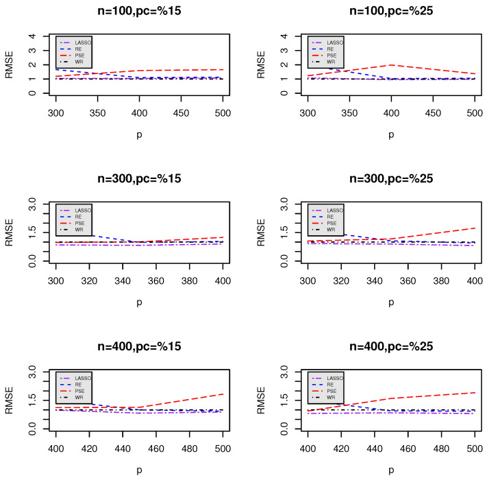 Figure 1
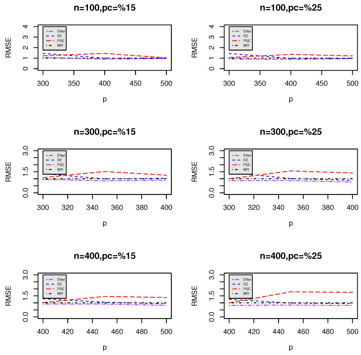 Figure 2
- —Natural Sciences and the Engineering Research Council of Canada (NSERC)
Peer Reviews
No public reviews on file for this paper yet. If you reviewed it on a platform where reviews are public (OpenReview, ICLR, NeurIPS, ICML), you can paste yours below so the community can read it here.
Videos
No videos yet. Explain this paper in a talk, walkthrough, or lecture? Add one.
Taxonomy
TopicsStatistical Methods and Inference
1. Introduction
High-dimensional data analysis, where the number of covariates frequently exceeds the sample size, has become a central research focus in contemporary statistics (see [1]). The applications of these methods span a broad range of fields, including genomics, medical imaging, signal processing, social science, and financial economics. In particular, high-dimensional regularized Cox regression models have gained traction in survival analysis (e.g., [2,3,4]), where these techniques help construct parsimonious (sparse) models and can outperform classical selection criteria such as Akaike’s information criterion [5] or the Bayesian information criterion [6].
The least absolute shrinkage and selection operation (LASSO) proposed by [7] remains one of the most popular approaches to high-dimensional regression, due to its computational efficiency and its ability to perform variable selection and parameter shrinkage simultaneously. Numerous extensions of LASSO, such as adaptive LASSO [8], elastic net [9], and scaled LASSO [10], have been developed to further refine estimation and prediction performance. In the context of Cox proportional hazards models, analogous methods—including the LASSO [4,11], the adaptive LASSO [12,13], and smoothly clipped absolute deviation (SCAD; [14])—have been widely examined. Interested readers may also consult [15,16,17,18] for recent advancements in high-dimensional Cox regression.
When , the focus is often on accurately recovering both the support (i.e., which covariates have nonzero effects) and the magnitudes of the nonzero regression coefficients. Although many penalized inference procedures excel at identifying “strong” signals (i.e., coefficients that are moderately large and thus easily detected), they may fail in adequately accounting for “weak” signals, whose effects may be small but nonzero. To formalize this, one can divide the index set into three disjoint subsets as follows: for strong signals, for weak signals, and for coefficients that are exactly zero. Standard estimation procedures that neglect weak signals risk introducing non-negligible bias, particularly when these weak signals are numerous.
In this paper, we tackle the bias induced by weak signals in high-dimensional Cox regression by adapting the post-selection shrinkage strategy proposed by [19]. Our key contribution is the development of a weighted ridge (WR) estimator, which effectively differentiates small, nonzero coefficients from those that are truly zero. We show that the resulting post-selection estimators dominate submodel estimators derived from standard regularization methods such as LASSO and elastic net. Moreover, under the condition for some , we establish the asymptotic normality of our post-selection WR estimator, thereby demonstrating its asymptotic efficiency. Through extensive simulations and real data applications, we illustrate that our method achieves substantial improvements in both estimation accuracy and prediction performance.
The remainder of this paper is organized as follows. Section 2 presents the model setup and the proposed post-selection shrinkage estimation procedure. In Section 3, we outline the asymptotic properties of our estimators. Section 4 provides a Monte Carlo simulation study, while Section 5 reports the results of applying our methodology to two real data sets. We conclude in Section 6 with a brief discussion of possible future research directions.
2. Methodology
2.1. Notation and Assumptions
In this section, we state some standard notations and assumptions, used throughout the paper. We use bold upper case letters for matrices and lower case letters for vectors. Moreover, denotes the matrix transpose and denotes the identity matrix. Design vectors, or columns of , are denoted by . The index set denotes the full model which contains all the potential variables. For a subset , we use for a subvector of indexed by , and for a submatrix of whose columns are indexed by . For a vector , we denote and . For any square matrix , we let and be the smallest and largest eigenvalues of , respectively. Given , we let and denote the maximum and minimum of a and b. For two positive sequences and , , if is in the same order as . We use to denote the indicator function; denotes the cumulative distribution function (cdf) of a non-central -distribution with degrees of freedom and non-centrality parameter . We also use to indicate convergence in distribution.
Let be the set of the indices of nonzero coefficients, with denoting the cardinality of . We assume that the true coefficient vector is sparse, that is . Without loss of generality, we partition the ( )-matrix as , where , and . For two matrices and , we define the corresponding sample covariance matrices by
Let be a submatrix of . Then, another partition can be written as . Let . Then, is a dimensional singular matrix with rank . We denote as all the positive eigenvalues of .
2.2. Signal Strength Regularity Conditions
We consider three signal strength assumptions to define three sets of covariates according to their signal strength levels as follows [19]:
- (A1) There exists a positive constant , such that for ;
- (A2) The coefficient vector satisfies for some , where for ;
- (A3) , for .
2.3. Cox Proportional Hazards Model
The proportional hazards (PH) model introduced by [20] is one of the most commonly used approaches for analyzing survival data. In this model, the hazard function for an individual depends on covariates through a multiplicative effect, implying that the ratio of hazards for different individuals remains constant over time. We consider a survival model with a true hazard function for a failure time T, given a covariate vector . We let C denote the censoring time and define and . Suppose we have n i.i.d. observations from this true underlying model, where represents the design matrix.
The PH model posits that the hazard function for an individual with covariates is
where is the vector of regression coefficients, and is an unknown baseline hazard function. Because does not depend on , one can estimate by maximizing the partial log-likelihood
where and is the risk set just prior to . Maximizing in (3) with respect to yields the estimator for the regression parameters.
2.4. Variable Selection and Estimation
Variable selection can be carried out by minimizing the penalized negative log-partial likelihood as follows:
where is a penalty function applied to each component of , and is a tuning parameter that controls the magnitude of penalization. We consider the following two popular methods:
- LASSO. The LASSO estimator follows (4) with an -norm penalty,
As increases, this penalty continuously shrinks the coefficients toward zero, and some coefficients become exactly zero if is sufficiently large. The theoretical properties of the LASSO are well studied; see [21] for an extensive review. 2. Elastic Net (ENet). The Elastic Net estimator implements (4) with the combined penalty
where . When , this reduces to the LASSO, and when , it becomes Ridge. Combining and penalties leverages the benefits of Ridge while still producing sparse solutions. Unlike LASSO, which can select n variables at most, ENet has no such limitation when .
2.4.1. Variable Selection Procedure for S1 and S2
We summarize the variable selection procedure for detecting the strong signals and the weak signals .
- Step 1 (detection of ). Obtain a candidate subset of strong signals using a penalized likelihood estimator (PLE). Specifically, consider
where penalizes each , shrinking weak effects toward zero and selecting the strong signals. The tuning parameter governs the size of the subset .
- Step 2 (detection of ). To identify , first solve a penalized regression problem with a ridge penalty only on the variables in . Formally,
where is a tuning parameter controlling the overall strength of regularization for variables in . We then define a post-selection weighted ridge (WR) estimator by
where is a thresholding parameter. The set is then
We apply this post-selection procedure only if . In particular, we set
2.4.2. Post-Selection Shrinkage Estimation
We now propose a shrinkage estimator that combines information from two post-selection estimators, and . Recall that
Define the post-selection shrinkage estimator for as
where , and is the restricted estimator obtained by maximizing the partial log-likelihood (3) over the set . The term is given by
using a generalized inverse if is singular.
To avoid over-shrinking when and have different signs, we define a positive shrinkage estimator via the convex combination
This modification is essential to prevent an overly aggressive shrinkage that might reverse the sign of estimates in .
3. Asymptotic Properties
In this section, we study the asymptotic properties of the the post-selection shrinkage estimators for the Cox regression model. To investigate the asymptotic theory, we need the following regularity conditions to be met.
(B1) for some .(B2) , where for in (A2).(B3) The existence of a positive definite matrix such that , where the eigenvalues of satisfy .(B4) Sparse Riesz condition: For the random design matrix , any with , and any vector , there exists such that holds with probability tending to 1.
The following theorems will make it easier to compute the asympotic distributional bias (ADB) and asympotic distributional risk (ADR) of the proposed estimators:
Theorem 1.Suppose that assumptions (A1)–(A3) and (B1)–(B4) hold. If we choose for some constant and defined in (10) with , then, in (9) satisfies
where , and α are defined in (A2), (B1), and (B2), respectively.
Theorem 2. Let for any vector satisfying . Suppose assumptions ( B1 )–( B4 ) hold. Consider a sparse Cox model with a signal strength under ( A1 )–( A3 ), and with . Suppose a pre-selected model such as is obtained with probability 1. If we choose in Theorem 1 with , then, we have the asymptotic normality,
Asymptotic Distributional Bias and Risk Analysis
In order to compare the estimators, we use the asymptotic distributional bias (ADB) and the asymptotic risk (ADR) expressions of the proposed estimators.
Definition 1. For any estimator and -dimensional vector , satisfying , the ADB and ADR of , respectively, are defined as
where . Let and
We have the following theorems on the expression of ADBs and ADRs of the post-selection estimators.
Theorem 3. Let be any -dimensional vector satisfying and . Under the assumptions ( A1) –( A3) , we have
where and .
See the Appendix A for a detailed proof.
Theorem **4.***Under the assumptions of Theorem 2, except (*A2) is replaced by , for , with , for some , we have
where and .
It can be observed that the theoretical results are different from Theorem 3 of [19]. Ref. [19] considered the ADR of PSE estimations for the linear model. In contrast, our Theorems 3 and 4 are used for the PSE with the Cox proportional hazards model, which are feasible estimations. From Theorem 4, we can compare the ADRs of the estimators.
Corollary 1. Under the assumptions in Theorem 4, we have
- If , then ;
- If and , then for .
Corollary 1 shows that the performance of the post-selection PSE is closely related to the RE. On the ond hand, if and are large, then the post-selection PSE tends to dominate the RE. Further, if a variable selection method generates the right submodel and , that is, , then, a post-selection likelihood estimator is the most efficient one compared with all other post-selection estimators.
Remark 1. The simultaneous variable selection and parameter estimation may not lead to a good estimation strategy when weak signals co-exist with zero signals. Even though the selected candidate subset models can be provided by some existing variable selection techniques when , the prediction performance can be improved by the post-selection shrinkage strategy, especially when an under-fitted subset model is selected by an aggressive variable selection procedure.
4. Simulation Study
In this section, we present a simulation study designed to compare the quadratic risk performance of the proposed estimators under the Cox regression model. Each row of the design matrix is generated i.i.d. from a distribution, where follows an autoregressive covariance structure, as follows:
In this setup, we consider the following true regression coefficients:
where the subsets and correspond to strong and weak signals, respectively. The true survival times are generated from an exponential distribution with parameter . Censoring times are drawn from a distribution, where c is chosen to achieve the desired censoring rate. We consider censoring rates of and , and we explore sample sizes .
We compare the performance of our proposed estimators against two well-known penalized likelihood methods, namely, LASSO and Elastic Net (ENet). We employ the R package glmnet to fit these penalized methods and choose the tuning parameters via cross-validation. For each combination of n and p, we run 1000 Monte Carlo simulations. Let denote either or after variable selection. We assess the performance using the relative mean squared error (RMSE) with respect to as follows:
An indicates that outperforms , and a larger RMSE signifies a stronger degree of superiority over .
Table 1 presents the relative mean squared error (RMSE) values for different regression methods—LASSO and Elastic Net (ENet)—under varying sample sizes (n), number of predictors (p), and censoring percentages (15% and 25%). The RMSE values are averaged over 1000 simulation runs. The table compares three estimators, , , and , providing insight into their performance under different settings.
Figure 1 and Figure 2 visualize the RMSE trends for different values of p when comparing LASSO (Figure 1) and ENet (Figure 2) against the proposed estimators (RE and PSE). The plots indicate how RMSE varies as p increases for different sample sizes (n) and censoring levels.
Key Observations and Insights
Superior performance of post-selection estimators: Across all combinations of n and p, the post-selection estimators ( and ) consistently demonstrate lower RMSEs compared to LASSO and ENet. This suggests that these estimators provide better predictive accuracy and stability. Impact of censoring percentage:
- When the censoring percentage increases from 15% to 25%, the RMSE values tend to increase across all methods, indicating the expected loss of predictive power due to increased censoring.
- However, the post-selection estimators maintain a more stable RMSE trend, demonstrating their robustness in handling censored data.
Effect of increasing predictors (p):
- As p increases, the RMSE for LASSO and ENet tends to rise, particularly under higher censoring rates.
- This trend suggests that LASSO and ENet struggle with larger feature spaces, likely due to their tendency to aggressively shrink weaker covariates.
- In contrast, the post-selection estimators show relatively stable RMSE behavior, indicating their ability to retain relevant information even in high-dimensional settings.
Impact of sample size (n) on RMSE stability:
- Larger sample sizes (n) generally lead to lower RMSE values across all methods.
- However, the gap between LASSO/ENet and the post-selection estimators remains consistent, reinforcing the advantage of the proposed methods even with more data.
Comparing LASSO and ENet:
- ENet generally has lower RMSE values than LASSO, particularly for small sample sizes, indicating its advantage in balancing feature selection and regularization.
- However, ENet still underperforms compared to post-selection estimators, suggesting that the additional shrinkage adjustments help mitigate underfitting issues.
To further compare the sparsity of the coefficient estimators, we also measure the False Positive Rate (FPR), as follows:
A higher FPR indicates that more non-informative variables are incorrectly included in the model, thereby complicating interpretation [22]. When does not contain any zero components, the FPR is undefined. Table 2 compares the performance of LASSO and Elastic Net (ENet) in selecting variables in a high-dimensional Cox model under and censoring. As sample size (n) increases, both methods select more variables, but false positive rates (FPR) also rise, especially for ENet. LASSO is more conservative, selecting fewer variables with a lower FPR, while ENet selects more but at the cost of higher false discoveries. Higher censoring slightly increases FPR, reducing selection accuracy. Overall, LASSO offers better false positive control, whereas ENet captures more variables but with increased risk of selecting irrelevant ones.
5. Real Data Example
In this section, we illustrate the practical utility of our proposed methodology on two different high-dimensional datasets.
5.1. Example 1
We first apply our method to a gene expression dataset comprising breast cancer patients, each with genes. All patients received anthracycline-based chemotherapy. Among these 614 individuals, there were 134 ( ) censored observations, and the mean time to treatment response was approximately years. Using biological pathways to identify important genes, Ref. [23] previously selected 29 genes and reported a maximum area under the receiver operating characteristic curve (AUC) of about . This relatively low AUC suggests limited predictive power when only using these 29 genes.
To improve upon these findings, we begin by performing an initial noise-reduction procedure on the data. This step helps remove potential outliers and irrelevant features, thereby enhancing the quality of the subsequent variable selection and estimation processes. We applied LASSO and Elastic Net (ENet) for gene selection. The results show that LASSO selected 14 genes, whereas ENet selected 12 genes. We then applied the proposed post-selection shrinkage estimators introduced in Section 2 to evaluate their performance compared to standard methods such as LASSO and Elastic Net. Table 3 shows the estimated coefficients from different estimators, along with the AUC at the bottom. It is evident that the PSE estimate has slightly improved the prediction performance.
5.2. Example 2
We now consider the diffuse large B-cell lymphoma (DLBCL) dataset of [24], which is also high-dimensional. This dataset was used as a primary example to illustrate the effectiveness of our proposed dimension-reduction method. It consists of measurements on 7399 genes obtained from 240 patients via customized cDNA microarrays (lymphochip). Each patient’s survival time was recorded, ranging from 0 to 21.8 years; 127 patients had died (uncensored) and 95 were alive (censored) at the end of the study. Additional details on the dataset can be found in [24].
To obtain the post-selection shrinkage estimators, we first selected candidate subsets using two variable selection approaches—LASSO and Elastic Net (ENet). All tuning parameters were chosen via 10-fold cross-validation. Table 4 shows the estimated coefficients from both LASSO and ENet for the setting . The AUC results indicate that generally outperforms and for both LASSO and ENet procedures. Notably, the ENet-based estimators appear more robust than those obtained via LASSO, underscoring the value of combining and penalties in high-dimensional survival analysis.
6. Conclusions
In this paper, we proposed high-dimensional post-selection shrinkage estimators for Cox’s proportional hazards models based on the work of [19]. We investigated the asymptotic risk properties of these estimators in relation to the risks of the subset candidate model, as well as the LASSO and ENet estimators. Our results indicate that the new estimators perform particularly well when the true model contains weak signals. The proposed strategy is also conceptually intuitive and computationally straightforward to implement.
Our theoretical analysis and simulation studies demonstrate that the post-selection shrinkage estimator exhibits superior performance relative to LASSO and ENet, in part because it mitigates the loss of efficiency often associated with variable selection. As a powerful tool for producing interpretable models, sparse modeling via penalized regularization has become increasingly popular for high-dimensional data analysis. Our post-selection shrinkage estimator preserves model interpretability while enhancing predictive accuracy compared to existing penalized regression techniques. Furthermore, two real-data examples illustrate the practical advantages of our method, confirming that its performance is robust and potentially valuable for a range of high-dimensional applications.
The reference list from the paper itself. Each links out to its DOI / PubMed record.
- 1Ahmed S.E. Big and Complex Data Analysis: Methodologies and Applications Springer Cham, Switzerland 2017
- 2Bradic J. Fan J. Jiang J. Regularization for Cox’s proportional hazards model with np-dimensionality Ann. Stat.2011393092312010.1214/11-AOS 91123066171 PMC 3468162 · doi ↗ · pubmed ↗
- 3Bradic J. Song R. Structured estimation for the nonparametric Cox model Electron. J. Stat.2015949253410.1214/15-EJS 1004 · doi ↗
- 4Gui J. Li H. Penalized Cox regression analysis in the high-dimensional and low-sample size settings with applications to microarray gene expression data Bioinformatics 2005213001300810.1093/bioinformatics/bti 42215814556 · doi ↗ · pubmed ↗
- 5Akaike H. A new look at the statistical model identification IEEE Trans. Autom. Control 19741971672310.1109/TAC.1974.1100705 · doi ↗
- 6Schwarz G. Estimating the dimension of a model Ann. Stat.1978646146410.1214/aos/1176344136 · doi ↗
- 7Tibshirani R. Regression shrinkage and selection via the Lasso J. R. Stat. Soc. Ser. B 19965826728810.1111/j.2517-6161.1996.tb 02080.x · doi ↗
- 8Zou H. The adaptive Lasso and its oracle properties J. Am. Stat. Assoc.20061011418142910.1198/016214506000000735 · doi ↗