Flow-Based Coronary Artery Bypass Graft Patency Metrics: Uncertainty Quantification Simulations to Guide Development
Sita Drost, Cornelis J. Drost

TL;DR
This study uses simulations to understand how uncertain current methods are for evaluating coronary artery bypass grafts, aiming to improve diagnostic accuracy.
Contribution
The paper introduces a novel diastolic resistance index and identifies key physiological factors affecting graft patency metrics.
Findings
Metrics quantifying diastolic dominance show highest sensitivity to graft stenosis.
Stenosis severity, cardiac period, and graft diameter are important parameters influencing patency metrics.
The novel diastolic resistance index is most sensitive to stenosis severity.
Abstract
Over time, transit time flow measurement (TTFM) has proven itself as a simple and effective tool for intra-operative evaluation of coronary artery bypass grafts (CABGs). However, metrics used to screen for possible technical error show considerable spread, preventing the definition of sharp cut-off values to distinguish between patent, questionable, and failed grafts. The simulation study presented in this paper aims to quantify this uncertainty for commonly used patency metrics, and to identify the most important physiological parameters influencing it. Uncertainty quantification was performed on a realistic multiscale numerical model of the coronary circulation, guided by Morris screening sensitivity analysis of a simpler, lumped-parameter model. Simulation results were qualitatively verified against results of a recent clinical study. Correspondence with clinical study data is…
Genes, proteins, chemicals, diseases, species, mutations and cell lines named across the full text — each resolved to its canonical identifier and authoritative record.
Click any figure to enlarge with its caption.
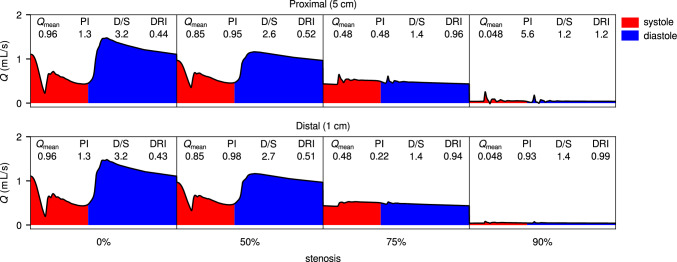 Figure 10
 Figure 11
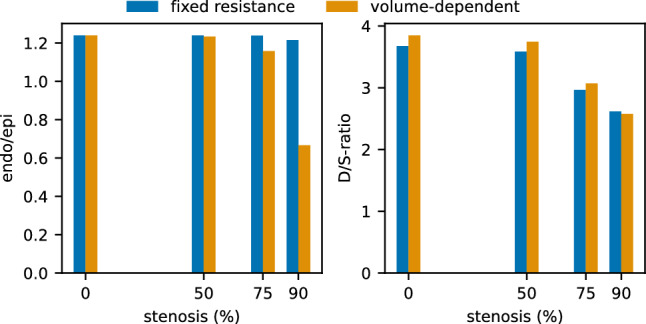 Figure 12
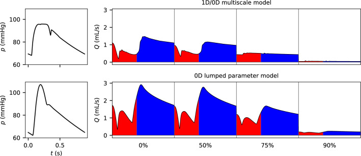 Figure 13
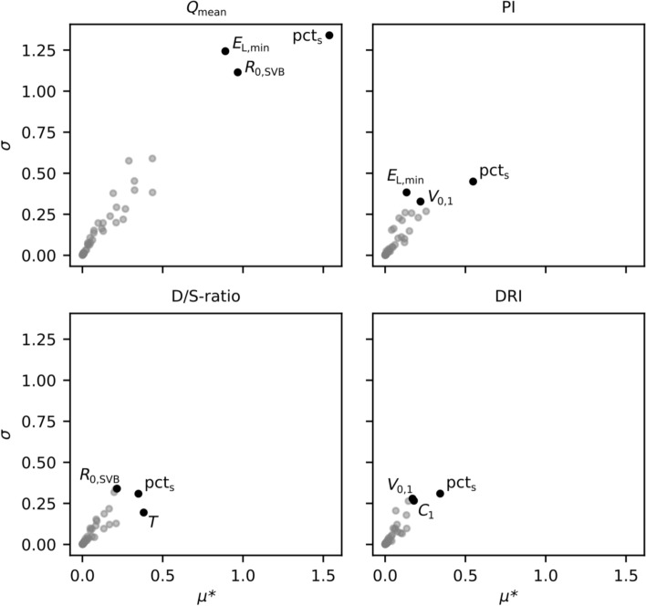 Figure 14
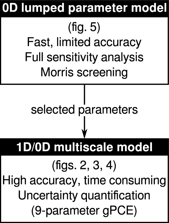 Figure 1
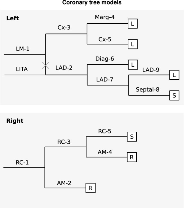 Figure 2
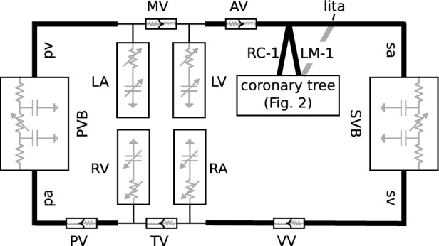 Figure 3
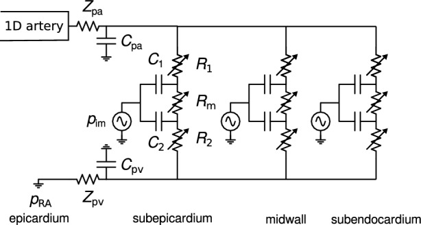 Figure 4
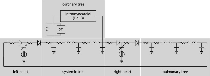 Figure 5
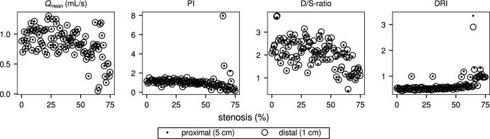 Figure 6
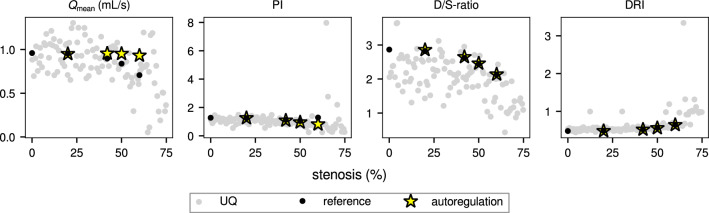 Figure 7
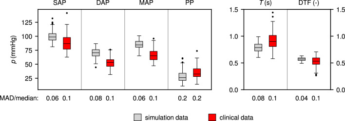 Figure 8
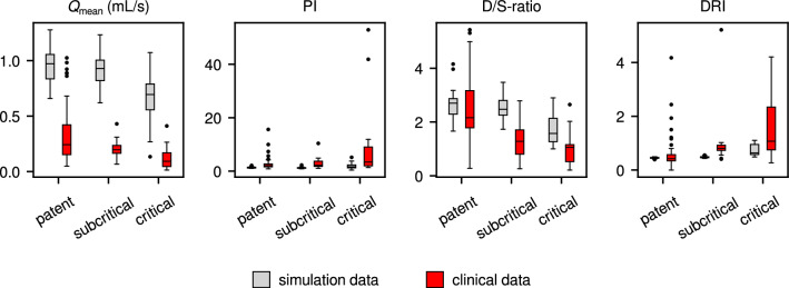 Figure 9
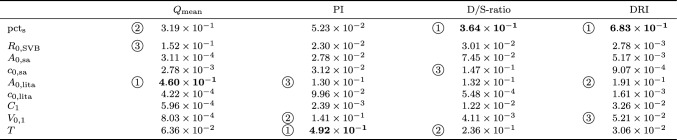 Figure 15
 Figure 16
Peer Reviews
No public reviews on file for this paper yet. If you reviewed it on a platform where reviews are public (OpenReview, ICLR, NeurIPS, ICML), you can paste yours below so the community can read it here.
Videos
No videos yet. Explain this paper in a talk, walkthrough, or lecture? Add one.
Taxonomy
TopicsCoronary Interventions and Diagnostics · Cardiac Valve Diseases and Treatments · Cardiac and Coronary Surgery Techniques
Introduction
Coronary artery bypass grafting (CABG) is a surgical procedure with a high rate of success. Still, a small percentage of grafts is reported to fail in the period up to 12 months post-surgery [1–3]. Reasons for graft failure are multitudinous, but among them is technical error. Therefore, to detect and correct technical error before chest closure, and thus reduce the risk of subsequent graft failure, intraoperative graft patency assessment is generally considered a valuable addition to the CABG surgery procedure [1, 4].
The gold standard for detecting flaws in a graft and its anastomosis is coronary angiography (CAG) [5, 6]. Angiography provides a precise assessment of vascular constriction; a qualitative assessment of the graft’s capacity to carry flow. The measurement involves relatively costly surgical equipment, requiring a trained operator and added surgical time, and is therefore not widely used for intraoperative patency assessment [1].
As a faster, simpler, and more affordable alternative, ultrasound transit time flow measurement (TTFM), as originally developed by Transonic Systems Inc. [7], is increasingly used for intraoperative CABG patency assessment [1–4]. By placing a hand-held flow probe around a newly created graft and holding it still for several seconds, the surgeon can accurately measure the time-varying flow rate through the graft. Deviations in the measured flow waveform can alert the surgeon of possible technical imperfections before the patient’s chest is closed. Presently in Japan, all CABG procedures include some form of flow-based patency assessment [8], while in the United States this percentage lies around 20% [4], the majority of which concerns off-pump CABG surgery. Also, the European 2018 ESC/EACTS Guidelines on Myocardial Revascularization [9] recommend TTFM to confirm graft patency.
The measured waveform is summarized in a number of patency metrics (see Sect. 2.1 for details), which were established over the years, based on clinical experience. Ideally, a (combination of) metric(s) should identify correctable technical errors in the newly constructed graft, independent of surgical confounders and patient parameters. However, in practice flow-based patency assessment is complicated by the many factors influencing the CABG flow waveform, such as target coronary, graft type (e.g. arterial or venous, single or sequential), competitive flow (resulting from incomplete occlusion of native coronary), autoregulation, quality of coronary microvasculature (resistance, compliance), but also patient parameters such as disease history, heart rate, cardiac index, blood pressure, and BMI [10]. As a result, the reliability of most flow-based patency metrics is high for the identification of severe stenoses, but decreases in case of subcritical stenoses [11].
Accounting for these factors in the metrics displayed on a TTFM flow monitor, or developing a novel metric, would require years of carefully controlled clinical studies. Development of novel metrics is ongoing [11–13], and generally is an empirical process, based on experience and clinical studies. To better guide such developments, a basic understanding is needed of the mechanisms determining the graft flow waveform and the factors influencing it. At the same time, such basic understanding is also expected to facilitate the user’s interpretation of a measured waveform on existing flow monitors. Therefore, as a complement to knowledge gained from clinical studies, we use computational fluid dynamics models to improve our understanding of the graft flow waveform.
The aim of our present study was to quantify uncertainty in the most commonly used patency metrics, and thus to assess their performance. To this end, we implemented a validated multi-scale numerical model of the coronary circulation [14–16], customized to include a CABG graft. To select parameters for uncertainty quantification using this model, Morris screening sensitivity analysis was performed using a simpler lumped-parameter model. Results were qualitatively verified against data from a recent clinical study by Takahashi et al. [11]. By providing an indication of the epistemic uncertainty associated with a certain metric, and of the key physiological parameters influencing this uncertainty, our approach should facilitate the design of effective clinical studies, and thus accelerate and focus the ongoing development of improved CABG patency metrics.
Sensitivity analysis and uncertainty quantification on a similar model, but applied to the pulmonary circulation, were reported by Colebank et al. [17], while Ge et al. [18] did a more limited, one-at-a-time (OAT) sensitivity analysis on a similar model of the coronary circulation. To the authors’ knowledge, this study is the first to specifically target flow-based CABG patency assessment.
Methods
To study the effects of stenosis in a graft, we use a realistic multi-scale numerical model of the coronary circulation (Figs. 2 and 4), embedded in a closed-loop cardiovascular model (Fig. 3), both developed by Mynard et al. [14, 16] and validated in-vivo [15]. Because, depending on stenosis severity and other parameter values, simulations with this model take between 5 and 100 h, performing a global sensitivity analysis is not feasible with this model. Instead, generalized polynomial chaos expansion (gPCE) uncertainty quantification was performed, with a limited number of parameters. To guide parameter selection, Morris screening sensitivity analysis was performed with a simpler – and thus, faster – lumped-parameter model (Fig. 5). The overall set-up our study is explained schematically in Fig. 1.Fig. 1. Flow chart representing the methods used in this study: first, Morris screening sensitivity analysis was performed, using a low-fidelity lumped parameter model. The parameters indicated as most influential by this analysis were used for generalized polynomial chaos expansion (gPCE) uncertainty quantification, using a realistic multiscale model.
Patency Metrics
In this study, the four most commonly used TTFM CABG patency metrics were included:
\documentclass[12pt]{minimal} \usepackage{amsmath} \usepackage{wasysym} \usepackage{amsfonts} \usepackage{amssymb} \usepackage{amsbsy} \usepackage{mathrsfs} \usepackage{upgreek} \setlength{\oddsidemargin}{-69pt} \begin{document}$$\begin{aligned}&\text {Mean\, flow\, rate:}&\quad &Q_\text {mean} = \frac{1}{T}\int _0^T Q(t) \textrm{d}t, \end{aligned}$$\end{document} \documentclass[12pt]{minimal} \usepackage{amsmath} \usepackage{wasysym} \usepackage{amsfonts} \usepackage{amssymb} \usepackage{amsbsy} \usepackage{mathrsfs} \usepackage{upgreek} \setlength{\oddsidemargin}{-69pt} \begin{document}$$\begin{aligned}&\text {Pulsatility\, index:}&\quad &\text {PI} = \frac{Q_\text {max} - Q_\text {min}}{Q_\text {mean}}, \end{aligned}$$\end{document} \documentclass[12pt]{minimal} \usepackage{amsmath} \usepackage{wasysym} \usepackage{amsfonts} \usepackage{amssymb} \usepackage{amsbsy} \usepackage{mathrsfs} \usepackage{upgreek} \setlength{\oddsidemargin}{-69pt} \begin{document}$$\begin{aligned}&\text {Diastolic/systolic\, ratio:}&\quad &\text {D/S-ratio} = \frac{|V_\text {dia}|}{|V_\text {sys}|}, \end{aligned}$$\end{document} \documentclass[12pt]{minimal} \usepackage{amsmath} \usepackage{wasysym} \usepackage{amsfonts} \usepackage{amssymb} \usepackage{amsbsy} \usepackage{mathrsfs} \usepackage{upgreek} \setlength{\oddsidemargin}{-69pt} \begin{document}$$\begin{aligned}&\text {Diastolic\, filling\, percentage:}&\quad &\text {DF\%} = \frac{|V_\text {dia}|}{|V_\text {tot}|}. \end{aligned}$$\end{document}Here, Q is flow rate, T is cardiac period, V is delivered blood volume (based on absolute flow rate), and subscripts max, min, tot, sys, and dia indicate maximum, minimum, total, systolic, and diastolic, respectively. DF% and D/S-ratio are directly related, as \documentclass[12pt]{minimal} \usepackage{amsmath} \usepackage{wasysym} \usepackage{amsfonts} \usepackage{amssymb} \usepackage{amsbsy} \usepackage{mathrsfs} \usepackage{upgreek} \setlength{\oddsidemargin}{-69pt} \begin{document}$$\text {DF\%} = 100 \times \text {D/S-ratio}/(1 + \text {D/S-ratio})$$\end{document} . Therefore, DF% was not included in the figures presented here.
Additionally, diastolic resistance index (DRI) was included:
\documentclass[12pt]{minimal} \usepackage{amsmath} \usepackage{wasysym} \usepackage{amsfonts} \usepackage{amssymb} \usepackage{amsbsy} \usepackage{mathrsfs} \usepackage{upgreek} \setlength{\oddsidemargin}{-69pt} \begin{document}$$\begin{aligned}&\text {Diastolic\, resistance\, index:}&\quad &\text {DRI} = \frac{\overline{p}_\text {dia}/|\overline{Q}_\text {dia}|}{\overline{p}_\text {sys}/|\overline{Q}_\text {sys}|}, \end{aligned}$$\end{document}where p is (central) pressure. This novel metric, developed by Transonic Systems Inc. (Ithaca, NY), was recently evaluated in a first clinical study by Takahashi et al. [11]. It incorporates both flow rate and pressure, and is related to D/S-ratio as:
\documentclass[12pt]{minimal} \usepackage{amsmath} \usepackage{wasysym} \usepackage{amsfonts} \usepackage{amssymb} \usepackage{amsbsy} \usepackage{mathrsfs} \usepackage{upgreek} \setlength{\oddsidemargin}{-69pt} \begin{document}$$\begin{aligned} \text {DRI} = \frac{\overline{p}_\text {dia}}{\overline{p}_\text {sys}}\frac{T_\text {dia}}{T_\text {sys}}\frac{1}{\text {D/S-ratio}}. \end{aligned}$$\end{document}It should be noted that, because DF% and D/S-ratio are computed using the absolute value of the flow rate, the same is done for DRI.
As explained in more detail in Appendix A, these patency metrics quantify different aspects of how the flow waveform changes in the presence of stenosis: \documentclass[12pt]{minimal} \usepackage{amsmath} \usepackage{wasysym} \usepackage{amsfonts} \usepackage{amssymb} \usepackage{amsbsy} \usepackage{mathrsfs} \usepackage{upgreek} \setlength{\oddsidemargin}{-69pt} \begin{document}$$Q_\text {mean}$$\end{document} quantifies the overall decrease in flow rate, while D/S-ratio, DF% and DRI capture the decrease in diastolic dominance. Finally, PI quantifies the combined effect of increasing capacitive flow proximal to the stenosis, and decreasing mean flow rate.
1D/0D Multiscale Model
The high-accuracy multiscale model that was used for gPCE uncertainty quantification consists of a model of the coronary circulation (Fig. 2), embedded in a closed-loop cardiovascular model (Fig. 3). Both the coronary tree model and the closed-loop cardiovascular model are made up of 1D segments representing the coronary arteries, and main systemic and pulmonary arteries and veins. The coronary artery segments are terminated with 0D lumped parameter intramyocardial perfusion models, and also the pulmonary and systemic vascular beds, and the heart were represented by 0D lumped parameter models.
In the lumped-parameter intramyocardial perfusion model (Fig. 4), the resistances in the sub-epicardial, mid-wall, and sub-endocardial layers depend on vascular volume. Incorporating volume-dependence of the compliances in these layers, as outlined by Algranati et al. [19], did not significantly alter the results, while it did increase the number of uncertain parameters in the model. Therefore, the compliances were assumed to be fixed in our study.
Following Suga et al. [20], maximum elastance in the heart model was set to be independent of cardiac period, while for diastole duration as a function of cardiac period the relation determined by Salvi et al. [21] was implemented.Fig. 21D/0D multiscale model: Diagrams detailing structure of left (top) and right (bottom) coronary tree models [14]. Labels correspond with segment names in Supplementary Material, boxes with L, R, S, represent instances of the lumped-parameter intramyocardial circulation model (Fig. 4) in the left and right ventricular wall and septum, respectively. The grey segment indicates a LITA graft, connected to the LAD (complete occlusion of LAD proximal to anastomosis is assumed in simulations with graft).Fig. 31D/0D multiscale model: Closed-loop cardiovascular model with coronary tree (adapted from Mynard et al. [16]). Boxes represent lumped-parameter models of microvascular beds, heart chambers, and valves, thick lines represent 1D segments, thin lines represent connections to lumped parameter models. LA/RA/LV/RV: left/right atrium/ventricle; MV: mitral valve, AV: aortic valve; TV: tricuspid valve; PV: pulmonary valve; VV: venous valve; PVB/SVB: pulmonary/systemic microvascular bed; sa: systemic artery; sv: systemic vein; pa: pulmonary artery; pv: pulmonary vein; LM-1: left main coronary artery; RC-1: right coronary artery, lita: left interior thoracic artery graft.Fig. 41D/0D multiscale model: Lumped-parameter model of intramyocardial circulation (adapted from Mynard et al. [16]). Intramyocardial pressure p \documentclass[12pt]{minimal} \usepackage{amsmath} \usepackage{wasysym} \usepackage{amsfonts} \usepackage{amssymb} \usepackage{amsbsy} \usepackage{mathrsfs} \usepackage{upgreek} \setlength{\oddsidemargin}{-69pt} \begin{document}$$_\text {im}$$\end{document} is generated by ventricular contraction, its influence is set to increase linearly with depth in the myocardial wall.
To this model a left internal thoracic artery (LITA) graft was added (indicated in grey in Fig. 2). Length and diameter of the LITA graft were based on data from the anatomically detailed arterial network (ADAN) model [22], resulting in a 20 cm long graft, with a radius tapering linearly from 0.142 cm to 0.0837 cm. This graft was anastomosed onto the left anterior descending (LAD) coronary artery, 0.3 cm distal to its origin from the left main (LM) coronary artery. Proximal to the anastomosis, the LAD was fully occluded. The origin of the LITA was placed on the systemic artery segment, 8 cm from the coronary ostia, so that the delay and distortion of its pressure waveform matched the ADAN data.
To the LITA graft, a stenosis was added at 1 cm from its distal end (model structure did not allow for stenosis to coincide with the anastomosis). Graft flow rate and pressure were monitored at two sites: 1 cm and 5 cm proximal of this stenosis. The former position corresponds with the flow probe position that is recommended by flow probe manufacturers, whereas the latter seems to better agree with clinical practice (based on informal discussions).
Stenosis was modeled following Young and Tsai [23]:
\documentclass[12pt]{minimal} \usepackage{amsmath} \usepackage{wasysym} \usepackage{amsfonts} \usepackage{amssymb} \usepackage{amsbsy} \usepackage{mathrsfs} \usepackage{upgreek} \setlength{\oddsidemargin}{-69pt} \begin{document}$$\begin{aligned} \Delta p_\text {s} = \frac{4 K_\text {v} \mu }{\pi D_0^3} Q_\text {s} + \frac{\rho K_\text {t}}{2 A_0^2}\left( \frac{A_0}{A_\text {s}} - 1\right) ^2 Q_\text {s}^2 + \frac{\rho K_\text {u} l_\text {s}}{A_0} \frac{\textrm{d}Q_\text {s}}{\textrm{d}t}, \end{aligned}$$\end{document}where \documentclass[12pt]{minimal} \usepackage{amsmath} \usepackage{wasysym} \usepackage{amsfonts} \usepackage{amssymb} \usepackage{amsbsy} \usepackage{mathrsfs} \usepackage{upgreek} \setlength{\oddsidemargin}{-69pt} \begin{document}$$\Delta p_\text {s}$$\end{document} is the pressure drop over the stenosis, \documentclass[12pt]{minimal} \usepackage{amsmath} \usepackage{wasysym} \usepackage{amsfonts} \usepackage{amssymb} \usepackage{amsbsy} \usepackage{mathrsfs} \usepackage{upgreek} \setlength{\oddsidemargin}{-69pt} \begin{document}$$D_0$$\end{document} and \documentclass[12pt]{minimal} \usepackage{amsmath} \usepackage{wasysym} \usepackage{amsfonts} \usepackage{amssymb} \usepackage{amsbsy} \usepackage{mathrsfs} \usepackage{upgreek} \setlength{\oddsidemargin}{-69pt} \begin{document}$$A_0$$\end{document} are the un-stenosed vessel diameter and cross-sectional area, respectively, \documentclass[12pt]{minimal} \usepackage{amsmath} \usepackage{wasysym} \usepackage{amsfonts} \usepackage{amssymb} \usepackage{amsbsy} \usepackage{mathrsfs} \usepackage{upgreek} \setlength{\oddsidemargin}{-69pt} \begin{document}$$A_\text {s}$$\end{document} and \documentclass[12pt]{minimal} \usepackage{amsmath} \usepackage{wasysym} \usepackage{amsfonts} \usepackage{amssymb} \usepackage{amsbsy} \usepackage{mathrsfs} \usepackage{upgreek} \setlength{\oddsidemargin}{-69pt} \begin{document}$$l_\text {s}$$\end{document} are the cross-sectional area and effective length of the stenosis, respectively, and \documentclass[12pt]{minimal} \usepackage{amsmath} \usepackage{wasysym} \usepackage{amsfonts} \usepackage{amssymb} \usepackage{amsbsy} \usepackage{mathrsfs} \usepackage{upgreek} \setlength{\oddsidemargin}{-69pt} \begin{document}$$K_\text {v}$$\end{document} , \documentclass[12pt]{minimal} \usepackage{amsmath} \usepackage{wasysym} \usepackage{amsfonts} \usepackage{amssymb} \usepackage{amsbsy} \usepackage{mathrsfs} \usepackage{upgreek} \setlength{\oddsidemargin}{-69pt} \begin{document}$$K_\text {t}$$\end{document} and \documentclass[12pt]{minimal} \usepackage{amsmath} \usepackage{wasysym} \usepackage{amsfonts} \usepackage{amssymb} \usepackage{amsbsy} \usepackage{mathrsfs} \usepackage{upgreek} \setlength{\oddsidemargin}{-69pt} \begin{document}$$K_\text {u}$$\end{document} are empirical constants related to viscous, turbulent, and inertial effects, respectively. The values of \documentclass[12pt]{minimal} \usepackage{amsmath} \usepackage{wasysym} \usepackage{amsfonts} \usepackage{amssymb} \usepackage{amsbsy} \usepackage{mathrsfs} \usepackage{upgreek} \setlength{\oddsidemargin}{-69pt} \begin{document}$$K_\text {t} = 1.52$$\end{document} and \documentclass[12pt]{minimal} \usepackage{amsmath} \usepackage{wasysym} \usepackage{amsfonts} \usepackage{amssymb} \usepackage{amsbsy} \usepackage{mathrsfs} \usepackage{upgreek} \setlength{\oddsidemargin}{-69pt} \begin{document}$$K_\text {u} = 1.2$$\end{document} are independent of stenosis shape, whereas \documentclass[12pt]{minimal} \usepackage{amsmath} \usepackage{wasysym} \usepackage{amsfonts} \usepackage{amssymb} \usepackage{amsbsy} \usepackage{mathrsfs} \usepackage{upgreek} \setlength{\oddsidemargin}{-69pt} \begin{document}$$K_\text {v}$$\end{document} depends on stenosis geometry as
\documentclass[12pt]{minimal} \usepackage{amsmath} \usepackage{wasysym} \usepackage{amsfonts} \usepackage{amssymb} \usepackage{amsbsy} \usepackage{mathrsfs} \usepackage{upgreek} \setlength{\oddsidemargin}{-69pt} \begin{document}$$\begin{aligned} K_\text {v} = 32 \frac{0.83 l_\text {s} + 1.64 D_\text {s}}{D_0}\left( \frac{A_0}{A_\text {s}}\right) ^2, \end{aligned}$$\end{document}with \documentclass[12pt]{minimal} \usepackage{amsmath} \usepackage{wasysym} \usepackage{amsfonts} \usepackage{amssymb} \usepackage{amsbsy} \usepackage{mathrsfs} \usepackage{upgreek} \setlength{\oddsidemargin}{-69pt} \begin{document}$$D_\text {s}$$\end{document} the diameter of the vena contracta. To study the effects of stenosis on graft flow, preliminary simulations were carried out, with 0, 50, 75, and 90% graft diameter reduction (see Appendix A).
Even though arterial pressure is known to be influenced by manipulation of the heart during off-pump CABG surgery [24–26], insufficient quantitative data were available to reliably include these changes in our simulations.
Finally, to limit model complexity, chamber interaction, as implemented by Mynard et al. [14, 16], and autoregulation, as implemented by Ge et al. [18], were not included in most simulations (however, see Sect. 2.6). Full model details and parameter values can be found in Appendix B.
The model was implemented in Python (https://www.python.org), using a finite difference flux-limited MacCormack scheme [27] to discretize the 1D flow equations. After checking for grid independence, a grid size of 0.1 cm was selected, with a time step of \documentclass[12pt]{minimal} \usepackage{amsmath} \usepackage{wasysym} \usepackage{amsfonts} \usepackage{amssymb} \usepackage{amsbsy} \usepackage{mathrsfs} \usepackage{upgreek} \setlength{\oddsidemargin}{-69pt} \begin{document}$$2\times 10^{-5}$$\end{document} s for simulations without stenosis, and progressively smaller for increasing stenosis severity. To simulate 10 cardiac periods, this resulted in simulation duration ranging from around 5 to 100 h (Dell Optiplex-7070 with Intel Core i7 processor).
0D Lumped Parameter Model
Because, based on earlier, exploratory simulations, most of the changes in the flow waveform as a result of stenosis were observed to originate from the lumped parameter stenosis model and the coronary microvasculature, a simplified model was created by connecting a single instance of the lumped parameter model of the intramyocardial vessels (Fig. 4) to the closed-loop lumped parameter cardiovascular circulation model of Avanzolini et al. [28] (Fig. 5). In a lumped parameter model, the geometric and mechanical properties of blood vessels are represented by lumped resistance, compliance, and (in larger vessels) inductance components. This way, a model comparable to that of Mantero et al. [29] was obtained, with which all essential features of the coronary flow waveform could be reproduced (see e.g. Fig. 13 in appendix C), including changes in myocardial perfusion as a function of diastolic time fraction [30] and perfusion pressure [19]. This model, with 39 parameters (including stenosis percentage), was implemented in OpenModelica (https://openmodelica.org/), and then exported as a functional mock-up unit (FMU), to be called from Python. With around 0.5 s to simulate 10 cardiac periods, this model allowed for global sensitivity analysis using Morris screening [31].Fig. 50D lumped parameter model: Lumped-parameter cardiovascular circulation model of Avanzolini et al. [28], with one instance of the intramyocardial circulation model of Mynard et al. [16] connected to it to represent coronary circulation. ST: stenosis model (3) [23], enabled by opening switch. See Appendix C for details.
Sensitivity Analysis
For the Morris screening sensitivity analysis, the Python package SALib [32, 33] was used, in which the efficient sampling strategy proposed by Ruano et al. [34] is implemented. For two parameters – stenosis percentage and subendocardial-subepicardial volume ratio [35] – a uniform distribution was assumed. For all other parameters, a normal distribution was assumed, truncated to mean \documentclass[12pt]{minimal} \usepackage{amsmath} \usepackage{wasysym} \usepackage{amsfonts} \usepackage{amssymb} \usepackage{amsbsy} \usepackage{mathrsfs} \usepackage{upgreek} \setlength{\oddsidemargin}{-69pt} \begin{document}$$\pm 2\times $$\end{document} standard deviation, with mean and standard deviation values guided by literature, such as the work of Charlton et al. [36]. If no standard deviation could be found in literature, a value of 25% of the mean of that parameter was assumed. For Morris screening, the parameter value distributions were sampled at \documentclass[12pt]{minimal} \usepackage{amsmath} \usepackage{wasysym} \usepackage{amsfonts} \usepackage{amssymb} \usepackage{amsbsy} \usepackage{mathrsfs} \usepackage{upgreek} \setlength{\oddsidemargin}{-69pt} \begin{document}$$p = 4$$\end{document} levels, and \documentclass[12pt]{minimal} \usepackage{amsmath} \usepackage{wasysym} \usepackage{amsfonts} \usepackage{amssymb} \usepackage{amsbsy} \usepackage{mathrsfs} \usepackage{upgreek} \setlength{\oddsidemargin}{-69pt} \begin{document}$$r = 50$$\end{document} trajectories were computed, resulting in a total of 2000 simulations (r was determined by increasing it in steps of 10, until the resulting 3 most influential parameters stopped changing). The patency metrics presented in the previous subsection, \documentclass[12pt]{minimal} \usepackage{amsmath} \usepackage{wasysym} \usepackage{amsfonts} \usepackage{amssymb} \usepackage{amsbsy} \usepackage{mathrsfs} \usepackage{upgreek} \setlength{\oddsidemargin}{-69pt} \begin{document}$$Q_\text {mean}$$\end{document} , PI, D/S-ratio, and DRI, were used as response variables. The influence of a parameter, quantified by the sensitivity measures \documentclass[12pt]{minimal} \usepackage{amsmath} \usepackage{wasysym} \usepackage{amsfonts} \usepackage{amssymb} \usepackage{amsbsy} \usepackage{mathrsfs} \usepackage{upgreek} \setlength{\oddsidemargin}{-69pt} \begin{document}$$\mu ^*$$\end{document} (mean of absolute elementary effects) and \documentclass[12pt]{minimal} \usepackage{amsmath} \usepackage{wasysym} \usepackage{amsfonts} \usepackage{amssymb} \usepackage{amsbsy} \usepackage{mathrsfs} \usepackage{upgreek} \setlength{\oddsidemargin}{-69pt} \begin{document}$$\sigma $$\end{document} (standard deviation of elementary effects), was summarized by \documentclass[12pt]{minimal} \usepackage{amsmath} \usepackage{wasysym} \usepackage{amsfonts} \usepackage{amssymb} \usepackage{amsbsy} \usepackage{mathrsfs} \usepackage{upgreek} \setlength{\oddsidemargin}{-69pt} \begin{document}$$\sqrt{\mu ^{*2} + \sigma ^2}$$\end{document} .
To ensure that the variables with uniform distribution did not have more influence just because the uniform distribution has higher entropy than the normal distribution, the sensitivity analysis was repeated with uniform distribution for all variables (with values in same range as in the corresponding truncated normal distribution). The influence of using all uniform distributions was found to be limited, and did not change the ranking of the most influential parameters.
Uncertainty Quantification
Apart from stenosis severity, the six most influential parameters resulting from Morris screening were selected for uncertainty quantification of the multiscale model. In addition to these parameters, the cross-sectional area and pulse wave speed of the systemic artery and graft were included. These were not part of the simplified lumped parameter model, but are known to influence the graft flow waveform and systemic pressure, respectively [15]. To limit the number of required simulations, only a model with LITA-LAD graft was analyzed, as this is the most commonly applied graft.
For the resulting parameters, a generalized polynomial chaos expansion (gPCE) was computed using Dakota [37]. Normal distributions were assumed for all parameter values but percentage stenosis, for which a uniform distribution was assumed.1 To prevent unrealistic values, normally distributed parameters were constrained to [mean value \documentclass[12pt]{minimal} \usepackage{amsmath} \usepackage{wasysym} \usepackage{amsfonts} \usepackage{amssymb} \usepackage{amsbsy} \usepackage{mathrsfs} \usepackage{upgreek} \setlength{\oddsidemargin}{-69pt} \begin{document}$$\pm 1.96\times $$\end{document} standard deviation] (i.e. 95% of probability density function). Using a maximum polynomial order of 2 (based on exploratory, coarse grid UQ with maximum polynomial order 4), and least-squares regression with a collocation factor of 2, this resulted in 110 simulations. As a part of the analysis, Dakota tested the quality of the gPCE using k-fold cross-validation, with 10 folds. To quantify the sensitivity of the flow-based metrics to each parameter, Sobol indices were computed directly from the resulting best-fitting gPCE [37].
Because parameters were assumed to vary independently, not all resulting flow and pressure waveforms were physiologically realistic. Using healthy subject values as a reference, as done by Charlton et al. [36], seemed too restrictive, as such values can hardly be expected to be representative of patients undergoing CABG surgery. Also, the availability of detailed physiological data of CABG surgery patients is insufficient to filter out unrealistic results. Therefore, all Morris screening results were retained, while from the gPCE results only the obviously erroneous results, with maximum pressure during diastole, were removed. This resulted in the removal of 6 out of 110 simulations (5%).
Autoregulation
In a normally functioning heart, autoregulation dilates or contracts the vessels in the myocardial wall, depending on flow demand [30]. As a result, blood flow to the myocardium, and subendocardial-to-subepicardial flow ratio, are not significantly affected in the presence of a coronary stenosis up to about 68% (90% area reduction, see e.g. Buss et al. [38]). Therefore, we expect the patency metrics to be affected by autoregulation.
As mentioned earlier, autoregulation was not included in the sensitivity analysis and uncertainty quantification simulations, to restrict computational cost. To still get an impression of the effects of autoregulation, four simulations with a stenosed LITA graft were run separately, in which intramyocardial resistance was tuned iteratively to maintain intramyocardial flow rate and endo-epi ratio at the un-stenosed level. These simulations were run with 20, 40, 50, and 60% stenosis, respectively.
Verification with Clinical Data
Dr. Takahashi of Nippon Medical School, Tokyo, Japan, kindly shared the raw data from his recent clinical study [11], which consisted of graft flow rate, radial artery pressure, and ECG waveforms, measured intraoperatively in 123 grafts, in 41 patients undergoing off-pump CABG surgery. From these data, \documentclass[12pt]{minimal} \usepackage{amsmath} \usepackage{wasysym} \usepackage{amsfonts} \usepackage{amssymb} \usepackage{amsbsy} \usepackage{mathrsfs} \usepackage{upgreek} \setlength{\oddsidemargin}{-69pt} \begin{document}$$Q_\text {mean}$$\end{document} , PI, D/S-ratio, DF%, and DRI were determined. Additionally, in all grafts percentage stenosis was measured postoperatively, using coronary computed tomography (CCT, for correspondence between measured stenosis grades, patency classes, and percentage diameter reduction, see Appendix, Table 8). The ECG signal was used for systole and diastole detection. Central systolic and diastolic pressure were estimated from the radial artery pressure waveform using the N-point moving average method proposed by Xiao et al. [39]. For measurement protocol, see Appendix, Sect. D.1.
For each patency metric, the median and interquartile range (IQR) for three different patency classes were compared between the clinical and simulated (1D/0D model) results. Because of the lack of detailed physiological data in CABG surgery patients, the 1D/0D model results were not expected to show quantitative agreement with the clinical results. Therefore, although the nonparametric Wilcoxon’s rank sum test was used to test for the significance of any observed differences, comparison was mostly qualitative, focusing more on trends than on exact agreement.
Results
Morris Screening and Uncertainty Quantification
Based on the results of the Morris screening analysis (see Appendix E), systemic vascular bed reference resistance \documentclass[12pt]{minimal} \usepackage{amsmath} \usepackage{wasysym} \usepackage{amsfonts} \usepackage{amssymb} \usepackage{amsbsy} \usepackage{mathrsfs} \usepackage{upgreek} \setlength{\oddsidemargin}{-69pt} \begin{document}$$R_\text {0,SVB}$$\end{document} (i.e. peripheral resistance), intramyocardial compliance arterial side \documentclass[12pt]{minimal} \usepackage{amsmath} \usepackage{wasysym} \usepackage{amsfonts} \usepackage{amssymb} \usepackage{amsbsy} \usepackage{mathrsfs} \usepackage{upgreek} \setlength{\oddsidemargin}{-69pt} \begin{document}$$C_1$$\end{document} , intramyocardial reference volume arterial side \documentclass[12pt]{minimal} \usepackage{amsmath} \usepackage{wasysym} \usepackage{amsfonts} \usepackage{amssymb} \usepackage{amsbsy} \usepackage{mathrsfs} \usepackage{upgreek} \setlength{\oddsidemargin}{-69pt} \begin{document}$$V_{0,1}$$\end{document} , and cardiac period T were selected for uncertainty quantification of the multi-scale model. Two additional parameters, maximum and minimum left ventricular elastance, were not selected for uncertainty quantification, as they were observed to mainly influence systemic pressure. Because systemic pressure is generally more influenced by cross-sectional area \documentclass[12pt]{minimal} \usepackage{amsmath} \usepackage{wasysym} \usepackage{amsfonts} \usepackage{amssymb} \usepackage{amsbsy} \usepackage{mathrsfs} \usepackage{upgreek} \setlength{\oddsidemargin}{-69pt} \begin{document}$$A_{0,\text {sa}}$$\end{document} and pulse wave velocity \documentclass[12pt]{minimal} \usepackage{amsmath} \usepackage{wasysym} \usepackage{amsfonts} \usepackage{amssymb} \usepackage{amsbsy} \usepackage{mathrsfs} \usepackage{upgreek} \setlength{\oddsidemargin}{-69pt} \begin{document}$$c_{0,\text {sa}}$$\end{document} of the systemic arteries [16] (not included in the lumped-parameter model), these parameters were selected instead. Finally, also the cross-sectional area and pulse wave velocity of the LITA graft, \documentclass[12pt]{minimal} \usepackage{amsmath} \usepackage{wasysym} \usepackage{amsfonts} \usepackage{amssymb} \usepackage{amsbsy} \usepackage{mathrsfs} \usepackage{upgreek} \setlength{\oddsidemargin}{-69pt} \begin{document}$$A_\text {0,LITA}$$\end{document} and \documentclass[12pt]{minimal} \usepackage{amsmath} \usepackage{wasysym} \usepackage{amsfonts} \usepackage{amssymb} \usepackage{amsbsy} \usepackage{mathrsfs} \usepackage{upgreek} \setlength{\oddsidemargin}{-69pt} \begin{document}$$c_\text {0,LITA}$$\end{document} , respectively, were included.
Scatter plots of the resulting patency metrics’ values vs. percentage stenosis, as monitored at 5 cm and 1 cm from the stenosis, are shown in Fig. 6. The observation by Jelenc et al. [40], that diastolic dominance is consistently lower when measured on the proximal side of the graft, is confirmed by our simulation results: D/S-ratio is on average 1.4% lower at 5 cm than at 1 cm from the stenosis (Wilcoxon signed rank test: significant difference, \documentclass[12pt]{minimal} \usepackage{amsmath} \usepackage{wasysym} \usepackage{amsfonts} \usepackage{amssymb} \usepackage{amsbsy} \usepackage{mathrsfs} \usepackage{upgreek} \setlength{\oddsidemargin}{-69pt} \begin{document}$$p < 0.001$$\end{document} ). Significant differences were similarly seen for DF% (0.4% lower), DRI (1.6% higher), and PI (2.7% lower).Fig. 6. Raw results of uncertainty quantification simulations, plotted as a function of percentage stenosis for each patency metric (black dots: 1 cm from stenosis at distal end of graft, open circles: 5 cm from stenosis at distal end of graft); for PI, D/S-ratio and DRI, differences between proximal and distal measurements are small but statistically significant.
Based on 10-fold cross-validation, linear expansion (i.e. order 1) was found to give the smallest error for all metrics. That is, even though the number of simulations allowed for second-order expansion, linear expansion was used for the gPCE. The Sobol indices computed from the gPCE, monitored at 5 cm from the stenosis, are listed in Table 1, with the most influential parameters printed in bold (see Appendix, Table 11 for results at 1 cm). Because linear expansion was used in all cases, the main and total Sobol indices are equal, so that only one value is given in the table.Table 1. Sobol indices from 9-parameter gPCE (5 cm from stenosis at distal end of graft); circled numbers indicate rankingpct \documentclass[12pt]{minimal} \usepackage{amsmath} \usepackage{wasysym} \usepackage{amsfonts} \usepackage{amssymb} \usepackage{amsbsy} \usepackage{mathrsfs} \usepackage{upgreek} \setlength{\oddsidemargin}{-69pt} \begin{document}$$_\text {s}$$\end{document} : percentage stenosis; \documentclass[12pt]{minimal} \usepackage{amsmath} \usepackage{wasysym} \usepackage{amsfonts} \usepackage{amssymb} \usepackage{amsbsy} \usepackage{mathrsfs} \usepackage{upgreek} \setlength{\oddsidemargin}{-69pt} \begin{document}$$R_\text {0,SVB}$$\end{document} : reference resistance systemic vascular bed; \documentclass[12pt]{minimal} \usepackage{amsmath} \usepackage{wasysym} \usepackage{amsfonts} \usepackage{amssymb} \usepackage{amsbsy} \usepackage{mathrsfs} \usepackage{upgreek} \setlength{\oddsidemargin}{-69pt} \begin{document}$$A_\text {0,sa}$$\end{document} : unstressed cross section systemic artery; \documentclass[12pt]{minimal} \usepackage{amsmath} \usepackage{wasysym} \usepackage{amsfonts} \usepackage{amssymb} \usepackage{amsbsy} \usepackage{mathrsfs} \usepackage{upgreek} \setlength{\oddsidemargin}{-69pt} \begin{document}$$c_\text {0,sa}$$\end{document} : unstressed wave speed systemic artery; \documentclass[12pt]{minimal} \usepackage{amsmath} \usepackage{wasysym} \usepackage{amsfonts} \usepackage{amssymb} \usepackage{amsbsy} \usepackage{mathrsfs} \usepackage{upgreek} \setlength{\oddsidemargin}{-69pt} \begin{document}$$A_\text {0,lita}$$\end{document} : unstressed cross section LITA graft; \documentclass[12pt]{minimal} \usepackage{amsmath} \usepackage{wasysym} \usepackage{amsfonts} \usepackage{amssymb} \usepackage{amsbsy} \usepackage{mathrsfs} \usepackage{upgreek} \setlength{\oddsidemargin}{-69pt} \begin{document}$$c_\text {0,lita}$$\end{document} : unstressed wave speed LITA graft; \documentclass[12pt]{minimal} \usepackage{amsmath} \usepackage{wasysym} \usepackage{amsfonts} \usepackage{amssymb} \usepackage{amsbsy} \usepackage{mathrsfs} \usepackage{upgreek} \setlength{\oddsidemargin}{-69pt} \begin{document}$$C_1$$\end{document} : intramyocardial compliance (arterial side); \documentclass[12pt]{minimal} \usepackage{amsmath} \usepackage{wasysym} \usepackage{amsfonts} \usepackage{amssymb} \usepackage{amsbsy} \usepackage{mathrsfs} \usepackage{upgreek} \setlength{\oddsidemargin}{-69pt} \begin{document}$$V_{0,1}$$\end{document} : reference intramyocardial volume (arterial side); T: cardiac period
Autoregulation
The results of the four autoregulation simulations, together with their reference results (i.e. same parameters, without autoregulation) are superimposed onto the raw uncertainty quantification results in Fig. 7. As intended, mean flow rate remains practically unchanged, while PI decreases slightly with stenosis severity, and both D/S-ratio and DRI are not noticeably affected by autoregulation.Fig. 7. Autoregulation results (yellow stars), and corresponding reference results (i.e. same parameter values, without autoregulation; black dots), plotted as a function of percentage stenosis (uncertainty quantification results are shown as grey dots in background; all results were monitored at 5 cm from stenosis at distal end of graft). As intended, autoregulation prevents \documentclass[12pt]{minimal} \usepackage{amsmath} \usepackage{wasysym} \usepackage{amsfonts} \usepackage{amssymb} \usepackage{amsbsy} \usepackage{mathrsfs} \usepackage{upgreek} \setlength{\oddsidemargin}{-69pt} \begin{document}$$Q_\text {mean}$$\end{document} from decreasing with increasing stenosis; the other metrics are only slightly (PI), or not noticeably (D/S-ratio, DRI) affected by autoregulation.
Verification Against Clinical Study Results
Box plots of hemodynamic parameters (systolic, diastolic, and mean arterial pressure in ascending aorta, with corresponding pulse pressure), and cardiac parameters (cardiac period, diastolic time fraction) are shown in Fig. 8. To quantify the variability of these parameters, the value of the median absolute deviation (MAD) relative to the median [41] is given under each box. The corresponding flow-based metrics’ values are shown in Fig. 9. The clinical study values of SAP, DAP and MAP are significantly lower than those in the simulation results (Wilcoxon’s rank-sum test), while PP and T are significantly higher. The variability of all hemodynamic and cardiac parameters is slightly higher in the clinical study results, or even much higher, as in the case of diastolic time fraction.
The 1D/0D simulation results for \documentclass[12pt]{minimal} \usepackage{amsmath} \usepackage{wasysym} \usepackage{amsfonts} \usepackage{amssymb} \usepackage{amsbsy} \usepackage{mathrsfs} \usepackage{upgreek} \setlength{\oddsidemargin}{-69pt} \begin{document}$$Q_\text {mean}$$\end{document} , D/S-ratio, and DRI show the same trend as the clinical results, but for PI, the trend is in opposite direction, and only the outliers suggest an increase with increasing stenosis severity. Furthermore, the clinical study values of \documentclass[12pt]{minimal} \usepackage{amsmath} \usepackage{wasysym} \usepackage{amsfonts} \usepackage{amssymb} \usepackage{amsbsy} \usepackage{mathrsfs} \usepackage{upgreek} \setlength{\oddsidemargin}{-69pt} \begin{document}$$Q_\text {mean}$$\end{document} are much lower than those in the simulations. All metrics’ values show a larger variability in the clinical study results.Fig. 8. Hemodynamic and cardiac parameters in 1D/0D simulation results (grey) and NMS clinical study results (red) [11]. SAP: systolic arterial pressure, DAP: diastolic arterial pressure, MAP: mean arterial pressure, PP: pulse pressure (mmHg, all in ascending aorta), T: cardiac period (s), DTF: diastolic time fraction (-); MAD/median quantifies parameter variability. Clinical study values of SAP, DAP and MAP are significantly lower than simulation results, PP and T are significantly higher.Fig. 9. Bar plots of flow-based metrics’ values in 1D/0D simulation results (grey) and NMS clinical study results (red), grouped per graft patency class (monitored at 5 cm from stenosis at distal end of graft). All metrics except PI show the same trend; except for \documentclass[12pt]{minimal} \usepackage{amsmath} \usepackage{wasysym} \usepackage{amsfonts} \usepackage{amssymb} \usepackage{amsbsy} \usepackage{mathrsfs} \usepackage{upgreek} \setlength{\oddsidemargin}{-69pt} \begin{document}$$Q_\text {mean}$$\end{document} , quantitative agreement is reasonable.
Discussion
Uncertainty quantification of the multiscale model, using generalized polynomial chaos expansion (gPCE), showed that for D/S-ratio and DRI, percentage stenosis is the most influential parameter, while for \documentclass[12pt]{minimal} \usepackage{amsmath} \usepackage{wasysym} \usepackage{amsfonts} \usepackage{amssymb} \usepackage{amsbsy} \usepackage{mathrsfs} \usepackage{upgreek} \setlength{\oddsidemargin}{-69pt} \begin{document}$$Q_\text {mean}$$\end{document} and PI, \documentclass[12pt]{minimal} \usepackage{amsmath} \usepackage{wasysym} \usepackage{amsfonts} \usepackage{amssymb} \usepackage{amsbsy} \usepackage{mathrsfs} \usepackage{upgreek} \setlength{\oddsidemargin}{-69pt} \begin{document}$$A_\text {0,lita}$$\end{document} and T are most important, respectively. Considering the inverse square relation between graft resistance and \documentclass[12pt]{minimal} \usepackage{amsmath} \usepackage{wasysym} \usepackage{amsfonts} \usepackage{amssymb} \usepackage{amsbsy} \usepackage{mathrsfs} \usepackage{upgreek} \setlength{\oddsidemargin}{-69pt} \begin{document}$$A_\text {0,lita}$$\end{document} , the strong influence of the latter on \documentclass[12pt]{minimal} \usepackage{amsmath} \usepackage{wasysym} \usepackage{amsfonts} \usepackage{amssymb} \usepackage{amsbsy} \usepackage{mathrsfs} \usepackage{upgreek} \setlength{\oddsidemargin}{-69pt} \begin{document}$$Q_\text {mean}$$\end{document} is understandable. The low sensitivity of PI to pct \documentclass[12pt]{minimal} \usepackage{amsmath} \usepackage{wasysym} \usepackage{amsfonts} \usepackage{amssymb} \usepackage{amsbsy} \usepackage{mathrsfs} \usepackage{upgreek} \setlength{\oddsidemargin}{-69pt} \begin{document}$$_\text {s}$$\end{document} found here might be explained by the fact that stenosis severity was limited to a maximum of 75% in our simulations, while PI only seems to start consistently increasing at pct \documentclass[12pt]{minimal} \usepackage{amsmath} \usepackage{wasysym} \usepackage{amsfonts} \usepackage{amssymb} \usepackage{amsbsy} \usepackage{mathrsfs} \usepackage{upgreek} \setlength{\oddsidemargin}{-69pt} \begin{document}$$_\text {s}$$\end{document} even higher than that (e.g. Fig. 10). For a metric to reliably detect stenosis, a high Sobol index for pct \documentclass[12pt]{minimal} \usepackage{amsmath} \usepackage{wasysym} \usepackage{amsfonts} \usepackage{amssymb} \usepackage{amsbsy} \usepackage{mathrsfs} \usepackage{upgreek} \setlength{\oddsidemargin}{-69pt} \begin{document}$$_\text {s}$$\end{document} is needed, preferably combined with low Sobol indices for other parameters of influence. During CABG surgery, \documentclass[12pt]{minimal} \usepackage{amsmath} \usepackage{wasysym} \usepackage{amsfonts} \usepackage{amssymb} \usepackage{amsbsy} \usepackage{mathrsfs} \usepackage{upgreek} \setlength{\oddsidemargin}{-69pt} \begin{document}$$A_\text {0,lita}$$\end{document} and T are routinely monitored so that it should be possible to account for their influence.
In the presence of autoregulation, intramyocardial arterioles will dilate to compensate for a reduction in perfusion pressure. As a result, stenoses with less than 90% area reduction (i.e. 68% diameter reduction) hardly affect mean flow rate and endo/epi ratio [38]. Therefore, in clinical practice, \documentclass[12pt]{minimal} \usepackage{amsmath} \usepackage{wasysym} \usepackage{amsfonts} \usepackage{amssymb} \usepackage{amsbsy} \usepackage{mathrsfs} \usepackage{upgreek} \setlength{\oddsidemargin}{-69pt} \begin{document}$$Q_\text {mean}$$\end{document} is generally observed to be useful for the detection of severe stenosis only. Our preliminary autoregulation simulations showed that also the utility of PI decreases. The diastolic dominance-based metrics D/S-ratio, DF% and DRI are hardly affected at all, suggesting that the influence of a shift in endo-epi ratio is only minor, and that the reduction in diastolic dominance with increasing stenosis is mainly caused by the flow rate dependence of stenosis pressure drop (3). This is further illustrated in appendix A.
The variability of most hemodynamic and cardiac parameter values in the uncertainty quantification results is slightly smaller, but reasonably close to that in the clinical study results used for comparison. Only for diastolic time fraction the variability is much smaller in the simulations than in the clinical study results. Systolic, diastolic and mean arterial pressure in the clinical study results are significantly lower than those in the simulation results, while pulse pressure and cardiac period are significantly higher. This may in part be caused by inaccuracies in estimating central pressure from peripheral pressure in the clinical study, but also the changes in hemodynamics during CABG surgery, due to anesthetics and manipulation of the heart, are expected to be of influence [24–26].
The much lower values of \documentclass[12pt]{minimal} \usepackage{amsmath} \usepackage{wasysym} \usepackage{amsfonts} \usepackage{amssymb} \usepackage{amsbsy} \usepackage{mathrsfs} \usepackage{upgreek} \setlength{\oddsidemargin}{-69pt} \begin{document}$$Q_\text {mean}$$\end{document} in the clinical study results are expected to be related to these lower pressure values, and perhaps the relatively small patient size in the (Japanese) clinical study. The combination of lower SAP, DAP, and MAP, with higher PP, may also explain the higher PI values in the clinical data. Overall, the metrics’ values show reasonable correspondence between clinical and simulation results, especially considering the fact that healthy subject parameter values were used in the simulation models. Plausible explanations for the larger variability and weaker correlation with stenosis severity of the clinical study results may be the variation in graft types and targets (single and sequential, arterial and venous grafts, to different target coronaries, possibly not all fully occluded). Additionally, measurement inaccuracy may have played a role, for example, in estimating central pressure from peripheral measurements, but also because of the sometimes large time lapse between surgery and postoperative CCT scan (median time interval from CABG surgery to CCT examination was 33 days; IQR 19–89 days; range 6–160 days).
More patient data are needed to reliably adapt the 1D/0D model to represent CABG surgery patients, and to estimate realistic ranges and distributions for the different model parameters.
Conclusions
Among the most commonly used patency metrics, D/S-ratio (and hence, DF%) displayed the highest sensitivity to stenosis severity, and the lowest sensitivity to the remaining physiological parameters in the study. The novel DRI showed even better performance in the simulation study, but not in the clinical results, suggesting that a more accurate central pressure estimate or measurement would be needed. All diastolic dominance-based metrics appear to be relatively insensitive to autoregulation.
As pointed out by Jelenc et al. [40], all metrics’ values except \documentclass[12pt]{minimal} \usepackage{amsmath} \usepackage{wasysym} \usepackage{amsfonts} \usepackage{amssymb} \usepackage{amsbsy} \usepackage{mathrsfs} \usepackage{upgreek} \setlength{\oddsidemargin}{-69pt} \begin{document}$$Q_\text {mean}$$\end{document} depend on flow probe position. However, in our results the difference between values measured proximally and distally was only \documentclass[12pt]{minimal} \usepackage{amsmath} \usepackage{wasysym} \usepackage{amsfonts} \usepackage{amssymb} \usepackage{amsbsy} \usepackage{mathrsfs} \usepackage{upgreek} \setlength{\oddsidemargin}{-69pt} \begin{document}$$1-2$$\end{document} % on average, and the corresponding Sobol indices are not significantly affected.
To further increase the practical relevance of the multiscale model used in this study, it may be extended to include different graft types and targets, autoregulation, and competitive flow. This would also allow further honing of flow-based patency metrics and their associated measurement protocol. Extending the model would require more computing power, further restriction of UQ complexity, or a more efficient model implementation. Additionally, a better understanding of hemodynamic and physiological changes during CABG surgery is needed for a more realistic model, using CABG patient parameters rather than healthy subject parameters. To this end, data from existing and new clinical studies may be used, for example, in combination with the approach adopted by Tran et al. [42].
Overall, from the angle of a company seeking to further improve and broaden the diagnostic strength of its flow-based CABG patency metrics and protocols, the method presented in this paper appears promising. Existing or newly-formulated metrics can be examined for their ability to separate the technical error conditions under control by the surgeon from the graft properties and patient conditions not under surgical control. Along with this, the statistical correlation between graft properties and patient conditions can be associated to the model variables, to define surgery/patient-specific modifiers to existing CABG patency metrics and thereby enhance their diagnostic precision. This can guide engineering development and ensuing clinical studies to validate efficacy and clinical outcomes.
The reference list from the paper itself. Each links out to its DOI / PubMed record.
- 1Lee, S.-W., J.-Y. Jo, W. Kim, D. Choi, and I. Choi. Patient and haemodynamic factors affecting intraoperative graft flow during coronary artery bypass grafting: an observational pilot study. Scientific Reports. 10, 2020. 10.1038/s 41598-020-69924-w.10.1038/s 41598-020-69924-w PMC 739510232737380 · doi ↗ · pubmed ↗
- 2Takahashi, K., Morota, T., Ishii, Y.: A novel transit-time flowmetric diastolic resistance index detects sub-critical anastomotic stenosis in coronary artery bypass grafting. JTCVS Techniques 17, 94–103 (2023) 10.1016/j.xjtc.2022.11.01310.1016/j.xjtc.2022.11.013PMC 993839236820345 · doi ↗ · pubmed ↗
- 3Ge, X., Z. Yin, Y. Fan, Y. Vassilevski, and F. Liang. A multi-scale model of the coronary circulation applied to investigate transmural myocardial flow. International Journal for Numerical Methods in Biomedical Engineering. 34, 2018. 10.1002/cnm.3123.10.1002/cnm.312329947132 · doi ↗ · pubmed ↗
- 4Spaan, J. A. E., Piek, J. J., and M. Siebes. Coronary circulation and hemodynamics. In: Sperelakis, N., Kurachi, Y., Terzic, A., and M. V. Cohen (eds.) Heart physiology and pathophysiology, 4th edn., 2001.
- 5Herman, J., and W. Usher. SA Lib An open-source python library for sensitivity analysis. The Journal of Open Source Software. 2(9), 2017. 10.21105/joss.00097.