Temporal and Spatial Coupling Methods for the Efficient Modelling of Dynamic Solids
Kin Fung Chan, Nicola Bombace, Indrajeet Sahu, Simone Falco, Nik Petrinic

TL;DR
This paper introduces efficient methods to reduce computational costs when modeling dynamic solids using finite elements.
Contribution
The novel contribution is a parameter-free coupling method combining multi-time-step and non-conforming mesh integration.
Findings
A multi-time-step integration algorithm reduces computational costs while maintaining accuracy.
The method achieves a speedup of over 12× compared to traditional single-time-step methods.
Interfaces between subdomains are resolved without additional degrees of freedom.
Abstract
This paper presents efficient coupling methods that accurately reduce the computational cost for modelling solids dynamically with finite elements. A multi-time-step integration algorithm is developed to leverage varying time steps throughout a domain. Interfaces between subdomains are resolved explicitly with the continuity of acceleration and tractions. A spatial coupling method is combined with multiple time steps, allowing for meshes that do not necessarily conform at their interfaces. The method avoids solving additional degrees of freedom at these interfaces, with parameter-free coupling operators defined between meshes. A speedup >12× is achieved in comparison to reference single-time-step methods.
Genes, proteins, chemicals, diseases, species, mutations and cell lines named across the full text — each resolved to its canonical identifier and authoritative record.
Click any figure to enlarge with its caption.
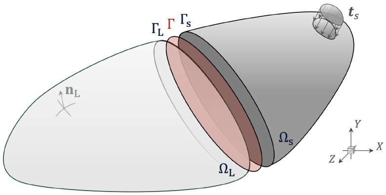 Figure 1
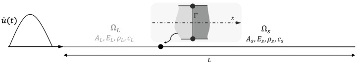 Figure 2
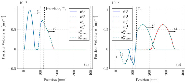 Figure 3
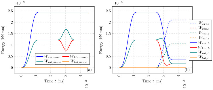 Figure 4
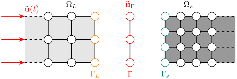 Figure 5
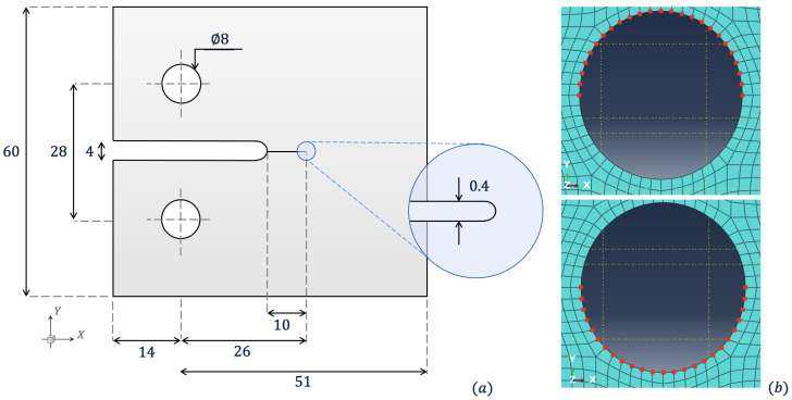 Figure 6
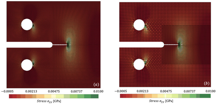 Figure 7
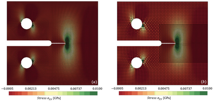 Figure 8
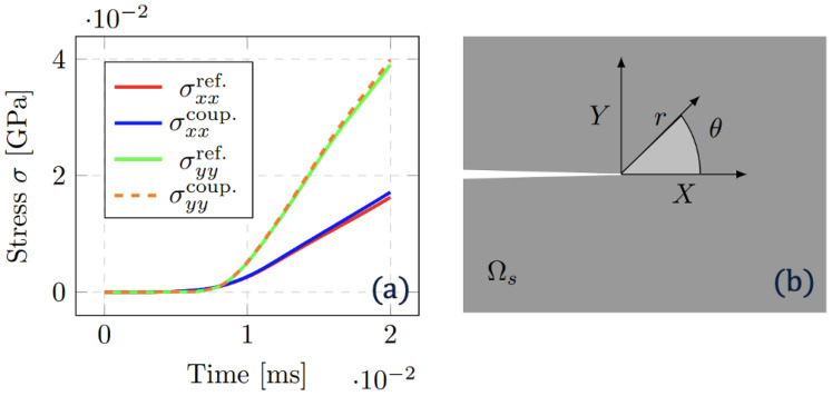 Figure 9
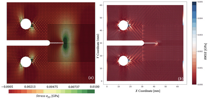 Figure 10
- —Engineering and Physical Sciences Research Council
Peer Reviews
No public reviews on file for this paper yet. If you reviewed it on a platform where reviews are public (OpenReview, ICLR, NeurIPS, ICML), you can paste yours below so the community can read it here.
Videos
No videos yet. Explain this paper in a talk, walkthrough, or lecture? Add one.
Taxonomy
TopicsAdvanced Numerical Methods in Computational Mathematics · Contact Mechanics and Variational Inequalities · Advanced Mathematical Modeling in Engineering
1. Introduction
The temporal and spatial discretisation of structural dynamic problems is directly related to the accuracy and computational cost of the explicit finite element method. Constrained by the Courant–Friedrichs–Lewy (CFL) condition, the critical time step, , is proportional to the element size, and inversely proportional to the dilatational wave speed [1]. This leads to simulations being restricted to of the element with the smallest size or highest wave speed. Initially referred to as subcycling, pioneering works allowed for the integration of multiple time steps in a single domain [2,3]. The coupling of various kinematic fields was explored, along with the stability of such algorithms [4,5]. Asynchronous variational integration is a non-trivial alternative, discretising the functional instead of the equations of motion [6]. The main drawback being its high complexity implementation. Heterogeneous asynchronous time integration extended methods to varying, non-integer and large time step ratios [7,8]. However, maintaining the continuity of kinematics at the interface remains a challenge, especially for all three fields [9]. In recent works, energy-conserving methods have been developed; however, they depart far from the CFL condition to resolve the interface conditions [10]. Spatially, non-matching mesh algorithms facilitate more flexible geometric modelling [11]. Nitsche’s method has shown to weakly enforce conditions on the interfaces of non-matching meshes without additional unknowns, but commonly suffers from sensitivity to parameters [12,13,14,15]. Following similar principles of weak continuity, Lagrange multipliers are called upon in the mortar-based methods [16,17,18,19,20]. These types of methods have proven to be very robust, however they struggle to fulfil the inf-sup stability condition, and incur a large computational cost with mapping master and slave nodes [21]. In comparison, the use of localised Lagrange multipliers introduces a frame that independently enforces compatibility constraints on each boundary [22,23,24,25,26,27]. However, as is common with other methods that introduce an additional discretised interface, the construction of this interface is neither trivial nor computationally cheap [28,29,30,31]. This brief review justifies the need for more efficient couplings, both temporally and spatially. Coupling algorithms that allow for varying time-step ratios, whilst stepping close to the CFL condition, concertedly those that solve for non-matching meshes, without increasing the degrees of freedom, remain a hot topic of research.
2. Governing Equations of Dynamic Solids
The problem of a solid body subject to impact is described through the partitioning of a domain as illustrated in Figure 1. The deformation is governed by the momentum balance equation acting on the solid domain :
where , , and denote the density, acceleration field, Cauchy stress tensor and body forces. Deformation is described at time for a specified constant . Updated Lagrangian formulations of a single body are found in the following [32,33,34]; here, we extend this to a partitioned formulation to solve multiple solid subdomains.
Defining multiple subdomains, we state is a solid body in an open region , with its boundary denoted . is partitioned into non-overlapping subdomains:
Starting from , for a two-subdomain partitioning, where and denote large and small subdomains. On the boundary of the two matching subdomains, , we enforce:
to ensure the continuity of acceleration and tractions , as well as enforcing Dirichlet and Neumann boundary conditions. The variational formulation of the dynamic equilibrium in Equation (1) can be described for both and as the following:
where we denote a variational velocity , in a space where , and as the rate of deformation. A discrete approximation of the variational form can be reduced to the following ordinary differential equations:
where for subdomains and , we sum, over a number of finite elements, and , in each subdomain:
The Lagrangian shape functions are represented by , with their derivatives denoted as . As is common within the explicit finite element method, is lumped for each subdomain, with and computed with vectors too. We elect to use the leapfrog time integration scheme to step through time, staggering the solution of each kinematic quantity such that:
noting that a diagonal mass matrix allows for a direct computation of acceleration. Velocity is computed on the half time step, with displacement found for each full time step. Next, we summarise the temporal coupling, enabled by multi-time-step (MTS) integration.
3. Multi-Time-Step Integration
Multi-time stepping enables partitioned subdomains and to integrate with and , respectively. However, to allow for this difference, special attention must be given to the solution of the interface . Crucially, the conditional stability of explicit methods requires an element’s time step to obey the CFL condition for a linear undamped system as follows:
Here, we represent as the critical time step, as the maximum eigenfrequency, as the characteristic length of an element e and the dilatational (longitudinal) wave speed.
3.1. Salient Multi-Time-Stepping Features
The asynchronous integration is enabled with three important groups of computations. The first is the explicit computation of the acceleration on the interface :
We define indicator matrices (vectors in 1-D) for each subdomain to identify the degrees of freedom on the interface of subdomains with dimensions for nodal number . These summations provide the ingredients for computing the interface acceleration:
where we compute at each large time step . The integration of the subdomains is controlled by the definition of the time-step ratios. Suppose the two subdomains begin at a similar point in time , where N and n are the small and large steps, respectively. The time after the maximum stable integration step (governed by the CFL condition) on each subdomain is referred to as the trial time , such that:
where for every , k small time steps elapse since the last point in time where subdomains are equal in time. Now we can define the current time-step ratio, , and next time-step ratio, for the advancement of with:
Starting from each common time step with the integration of , the number of small time steps is determined by the evaluation of time-step ratios and . If the condition of or ( and ) is satisfied, further steps on can proceed before integrating over . As a consequence of subdomains integrating over their own respective time step, we ensure that the proposed method still finds a common time between all subdomains. Following the small trial time exceeding the large trial time , the method computes two additional ratios and . These denote the reduction factors required to maintain the subdomains in synchronisation where . Hence:
Through computing on both subdomains, we can compare reduction factors, such that:
where we look to reduce the time step of the subdomain closest to the CFL condition. In the following section, we summarise the multi-time-stepping algorithm, with each of these key features, as well as its implementation.
3.2. Summary of Temporal Algorithm
We provide an overview of the method required to integrate and with and . It shows a single large step N, exemplifying each of the features mentioned above. Note that is used for when , and computation of in Equation (15) is only required at for a mass-conserving problem. One full loop of the procedure times is followed, with the subdomain synchronised after each large step N. The proposed method is implemented in an open-source python code, found in the following repository: https://github.com/kinfungchan/multi-time-step-integration (accessed on 9 December 2024) [35]. It contains re-implementations of methods from the literature for the two-subdomain cases [9,10]. Whilst we depict the case of just two subdomains, the Algorithm 1 can be extended to multiple by processing subdomains as pairs. Algorithm 1 Summary of Algorithm for Coupling in Time from N to
- 1:procedure a two-subdomain multi-time integration step
- 2: while or ( and ) do
- 3: Integrate subdomain with and compute force vectors over
- 4: Compute trial times , and time step ratios ,
- 5: Compute time step reduction factors
- 6: if then
- 7:
- 8: else
- 9:
- 10: Integrate subdomain with and recompute force vectors over
- 11: Recompute trial times , and time step ratios ,
- 12: Integrate subdomain with and compute force vectors over
- 13: Compute interface acceleration with Equations (15)–(17) for next time step
- 14: Recompute trial times , and time step ratios ,
3.3. Numerical Examples in Time
We present a numerical example in 1-D, with the elastic wave propagation through a heterogeneous bar. Suppose the domain is split into two subdomains and of similar discretisation, with isotropic elastic properties of GPa, GPa and kgmm^−3^. These material properties result in a non-integer , where the time-step ratio is solely driven by the dissimilar material properties. Figure 2 depicts the bar configuration. The velocity boundary condition is applied to at with ms^−1^, where we define a half sine wave with a frequency of rads^−1^. The difference in material impedance results in a portion of the incident wave being transmitted and the remainder reflected in the opposite direction.
In Figure 3, a comparison between the coupled solution ( with ) and the monolithic (single-time-step) solution is presented at four separate time stamps. The multi-time-step solution solves and over and , whereas is limited by . Consequently, for , our method reduces the number of integration steps on by half. From prescription of the full wave at , through to the transmission and reflection of the wave at , the MTS solution aligns very well with the single-time-step solution, despite halving the number of large time steps. This reduction in computational effort is even more prominent for highly heterogeneous configurations, as well as variance in spatial discretisation.
For the above simulation, we also compute the energy components, at each small time step, of each subdomain with the following:
where n can be interchanged with N when evaluating . The balance of energy can be evaluated in a similar way to the works of Neal and Belytschko [3], with the following:
In Figure 4, we show each of the components of energy and its overall balance. For both monolithic and multi-time-step solutions, a smooth transition of energy is observed as the wave interacts with . Remarkably, as the temporal coupling is enforced, the for both and is of the order kNmm, significantly below each of the components at kNmm. This numerical example captures the propagation of a smooth pulse; however, severe loading cases, highly heterogeneous domains, and 3-D problems, with further details are provided in the following work [35].
4. Solving Non-Matching Meshes
The problem of non-matching meshes is commonly found when simulating the dynamical behaviour of solids. We present an algorithm, combined with multi-time stepping, that relaxes the constraint of these conforming nodes, allowing for a coarser representation of a subdomain to be utilised, hence reducing the computational overhead.
4.1. Combined Spatial and Temporal Coupling
The following section follows on from the governing equations defined in Section 2; however, we now allow for the non-overlapping interface to consist of two non-matching spatial discretisations. Their compatibility is maintained such that:
where positions use an incidence matrix, such that and for each subdomain, and the externally assembled interface contains to describe the common boundary between the subdomains. The total virtual power can be summated for two subdomains to give , where a general form is obtained:
where variations in velocity coupling force on the interface and are accounted for. and are interpolation (or prolongation) and incidence operators ( to ), respectively. To map to the interface, we describe this spatial coupling operator in more detail:
with dimensions determined by and , as the number of nodes on the interface of the subdomain and the number of nodes on the interface , respectively. Therefore, interpolates using Lagrangian shape functions for the two subdomains and :
where is viewed as a dirac Delta function for coincident nodes. It is convenient to define a restriction operator as the transpose of , to map both forces and mass from subdomain interfaces and onto . The summation on the interfaces now becomes:
where we compute mass , internal force and external force to allow for the explicit computation of in Equation (17) to be recalled. These operators are analogous to concepts in multigrid methods and localised Lagrange multipliers (LLMs) [36,37]. Subsequently, we map from , back to the subdomains’ interfaces:
We illustrate a non-matching mesh in Figure 5 and compute its operators through exemplifying a linear isoparametric mapping in 2-D, where is discretised with line elements to depict the simplicity of this coupling.
For the interpolation matrix, we elucidate that from to the mapping is simply one-to-one and will always take the form of an identity matrix , whereas requires computation of the shape functions:
where, for this example case, it can also be shown that the restriction is the transpose of the interpolation. The interface is assumed to share the same geometrical description on both subdomain interfaces and , without overlap or separation. The spatial and temporal methods are combined to give the following Algorithm 2: Algorithm 2 Summary of Non-Matching Mesh Algorithm with Multi-Time Stepping
- 1:procedureintegrate a two-domain non-matching mesh with MTS
- 2: while or ( and ) do
- 3: Compute with operator in Equation (34) on
- 4: Integrate small domain and compute vectors
- 5: Compute trial times , and time step ratios ,
- 6: Compute time step reduction factors
- 7: if then
- 8:
- 9: else
- 10:
- 11: Compute with operator in Equation (34) on
- 12: Integrate small domain and compute vectors
- 13: Recompute trial times , and time step ratios ,
- 14: Compute with operator in Equation (34) on
- 15: Integrate large domain and compute vectors
- 16: Summate kinetics with to find and with Equation (31)–(33)
- 17: Compute trial times , and time step ratios ,
4.2. Numerical Examples in Space and Time
The following numerical study looks to represent the stress gradients prior to fracture in a compact-tension (CT) specimen test, utilising a similar geometry to the literature [38,39]. Figure 6a portrays the geometry modelled in the following example. As the specimen is loaded, stress concentrates about the specimen’s crack tip. We apply a ramped velocity boundary condition on nodes that create a semicircle for upper and lower pins, as shown in Figure 6b, with a maximum magnitude of 0.2 ms^−1^. Whilst uniformly distributed velocities are applied to each of the nodes in the pins, to replicate the contact pressure on the pins, methods such as those applied by Triclot et al. should be considered [40]. Material properties are similar to alumina with GPa, kgmm^−3^ and Poisson’s ratio . We model the CT specimen with three simulations: one using a fine mesh throughout the entire domain, one coupling a coarse and fine mesh with a single , and another with and integrating with multiple time steps and , respectively. Structured meshes are used in all cases where an element size of mm for fine and 1 mm for coarse. All simulations use , running for a maximum of ms.
In Figure 7 and Figure 8, we plot the stress contours at ms and ms, respectively, where the stress concentration can be visualised at the crack tip of the specimen. Figure 7a and Figure 8a capture the reference mesh, whilst Figure 7b and Figure 8b capture the spatially coupled mesh on a single time step . Figure 8 accurately predicts maximum stresses of 0.0396 GPa vs. 0.0410 GPa for reference against non-matching mesh.
Further quantification on the performance of the non-matching mesh algorithm can be made with the evaluation of stress intensity factors, near the crack tip. Utilising the stress extrapolation method, stress values in the vicinity of the crack tip can be used to simultaneously solve for in-plane and shear factors [41,42]. In rectangular coordinates, these are given as follows:
where r represents the radial distance from the crack, and the angle relative to the crack plane. Whilst J-integral and virtual crack closure techniques (VCCTs) have been developed for more accurately evaluating K, here the consistency in the method for both reference and coupled solution proves a sufficient comparison [43,44]. The stress and in the nearest element to the crack correspond to Figure 9a where strong alignment between spatially coupled and reference solution can be observed. In Figure 9b, the analysis computes and with mm, , mm and with the slight variation in the spatial discretisation of and summarising in Table 1. and compute a difference of 3.5% and 6.3% in value when comparing uncoupled and coupled solutions. This is deemed reasonable granted the approximation of the stress extrapolation method. For future comparisons, the contribution of multiple Gauss integration points could be considered with the aforementioned J-integral or VCCT methods.
Now with multi-time stepping, and step with ms and ms, producing a time-step ratio . Through combining spatial and temporal coupling, we observe similar (< GPa) results in distribution, as seen in Figure 10a. The difference in the coupled simulations is captured via Figure 10b, where the root mean square error (RMSE) is plotted. The stress is linearly interpolated for the non-matching mesh to allow for comparison of stress on the coarse mesh’s Gauss points. The couplings capture nearly the entire specimen within a <5% error. Considerable error is located around the circumference of the pins, where the chequerboard pattern indicates potential hourglassing in . To mitigate such issues, higher order or fully integrated elements could be used. However, in the presented results, we note that no hourglass control methods have been applied for fair comparison of the reference and coupled solutions. The other portion of error can be seen in the far right of the specimen in Figure 10; however, like the pins, these Gauss points reside far from the area of interest at the crack tip. To avoid such errors, a smaller element size would be required in ; however, this raises the trade-off between accuracy and computational efficiency. As per the temporal coupling, an energy balance in each of the two subdomains was achieved kNmm, orders of magnitude below individual components of energy. The computational efficiency is summarised with speedup achieved utilising both couplings, as presented in Table 2. Whilst a modest speedup is achieved with non-matching meshes, an even larger efficiency is found with coupling in both space and time. Considering that coupling with non-matching meshes and combined coupling in space and time result in similar accuracy, the addition of multi-time stepping to these simulations seems obvious.
5. Conclusions
We present coupling methods for the dynamic modelling of solids with explicit finite elements, temporally and spatially. When modelling composites, constituents have varying dilatational wave speeds, hence different time steps. Integrating over the smallest time step can prove highly inefficient, hence the need for multi-time stepping. Our method allows partitions of a domain to solve with their own respective time step, regardless of time-step ratio, hence reducing computational overhead. The method avoids solving a system of equations on the interface, unlike many of the methods that employ Lagrange multipliers. The stability of the method is assessed through evaluation of the subdomains’ energy balance. Very-high-frequency content or variations in motion below the time step of elements on the interface could result in spurious oscillations being generated. This potential limitation promotes the development of adaptive multi-time-stepping schemes that maintain the stability of the interface, withstanding high-frequency stress waves.
The addition of the coupling in space solves the issue of non-matching meshes so that small element sizes are only required in regions of interest. Coupling operators are easily implemented, without increasing the degrees of freedom on the interface. The method avoids the storage of large sparse matrices, reducing computational memory requirements. Ongoing work addresses the spatial coupling with quadrilateral non-matching interfaces in 3-D domains [45]. Numerical examples capture an increase in efficiency with stress wave propagation in a heterogeneous bar, and the modelling of a compact-tension specimen. Both couplings in time and space reduce computational runtimes when compared to their monolithic simulation, especially when combined. Limitations that concern the combination of spatial and temporal coupling include the computation of operators and solely at . Whilst this suffices for the benchmarks shown, for larger deformations this assumption is likely to require further development. Geometric representations of a non-matching that are non-planar have still yet to be explored. This proves an important topic as these couplings are applied to real-world multi-scale problems.
Future work looks at the coupling between macro- and meso-scale meshes [46,47,48], with adaptivity a clear necessity for these multi-scale couplings [49]. Whilst linear elasticity is a fair assumption for the rates of deformation demonstrated, other constitutive models should be investigated to evaluate the performance of the couplings, with further reductions in time steps and element distortion. In parallel, experimental fields that require efficiently capturing wave propagation with explicit finite elements are widespread [50,51]. Other coupling opportunities are plentiful when considering dynamic applications; the modelling of contact [14,16], composite fractures [38,39], fluid–structure interactions [13,27], and other impact engineering scenarios are just a few worth mentioning.
The reference list from the paper itself. Each links out to its DOI / PubMed record.
- 1Courant R. Friedrichs K. Lewy H. On the partial difference equations of mathematical physics IBM J. Res. Dev.19671121523410.1147/rd.112.0215 · doi ↗
- 2Hughes T.J. Liu W.K. Implicit-explicit finite elements in transient analysis: Implementation and numerical examples J. Appl. Mech. Trans. ASME 19784537537810.1115/1.3424305 · doi ↗
- 3Neal M.O. Belytschko T. Explicit-explicit subcycling with non-integer time step ratios for structural dynamic systems Comput. Struct.19893187188010.1016/0045-7949(89)90272-1 · doi ↗
- 4Daniel W.J.T. Analysis and implementation of a new constant acceleration subcycling algorithm Int. J. Numer. Methods Eng.1997402841285510.1002/(SICI)1097-0207(19970815)40:15<2841::AID-NME 193>3.0.CO;2-S · doi ↗
- 5Daniel W.J.T. A partial velocity approach to subcycling structural dynamics Comput. Methods Appl. Mech. Eng.200319237539410.1016/S 0045-7825(02)00518-2 · doi ↗
- 6Lew A. Marsden J.E. Ortiz M. West M. Variational time integrators Int. J. Numer. Methods Eng.20046015321210.1002/nme.958 · doi ↗
- 7Combescure A. Gravouil A. A numerical scheme to couple subdomains with different time-steps for predominantly linear transient analysis Comput. Methods Appl. Mech. Eng.20021911129115710.1016/S 0045-7825(01)00190-6 · doi ↗
- 8Gravouil A. Combescure A. Brun M. Heterogeneous asynchronous time integrators for computational structural dynamics Int. J. Numer. Methods Eng.201510220223210.1002/nme.4818 · doi ↗