Structural Causes of Pattern Formation and Loss Through Model-Independent Bifurcation Analysis
Liam D. O’Brien, Adriana T. Dawes

TL;DR
This paper introduces a new method to analyze how cell patterns form during development using minimal assumptions about cell communication and signaling.
Contribution
The novel contribution is a model-independent ODE framework that predicts stable cell patterns based on intercellular and intracellular signaling assumptions.
Findings
Global intercellular communication networks determine possible emergent patterns in a generic system.
Adding constraints on local intracellular signaling leads to a single stable pattern based on network features.
The framework allows inferring unknown signaling interactions by analyzing tissue-level patterns.
Abstract
During development, precise cellular patterning is essential for the formation of functional tissues and organs. These patterns arise from conserved signaling networks that regulate communication both within and between cells. Here, we develop and present a model-independent ordinary differential equation (ODE) framework for analyzing pattern formation in a homogeneous cell array. In contrast to traditional approaches that focus on specific equations, our method relies solely on general assumptions about global intercellular communication (between cells) and qualitative properties of local intracellular biochemical signaling (within cells). Prior work has shown that global intercellular communication networks alone determine the possible emergent patterns in a generic system. We build on these results by demonstrating that additional constraints on the local intracellular signaling…
Genes, proteins, chemicals, diseases, species, mutations and cell lines named across the full text — each resolved to its canonical identifier and authoritative record.
Click any figure to enlarge with its caption.
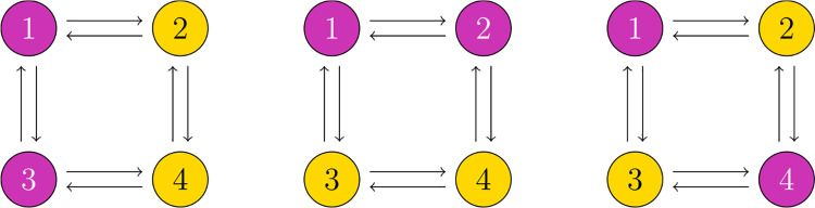 Figure 1
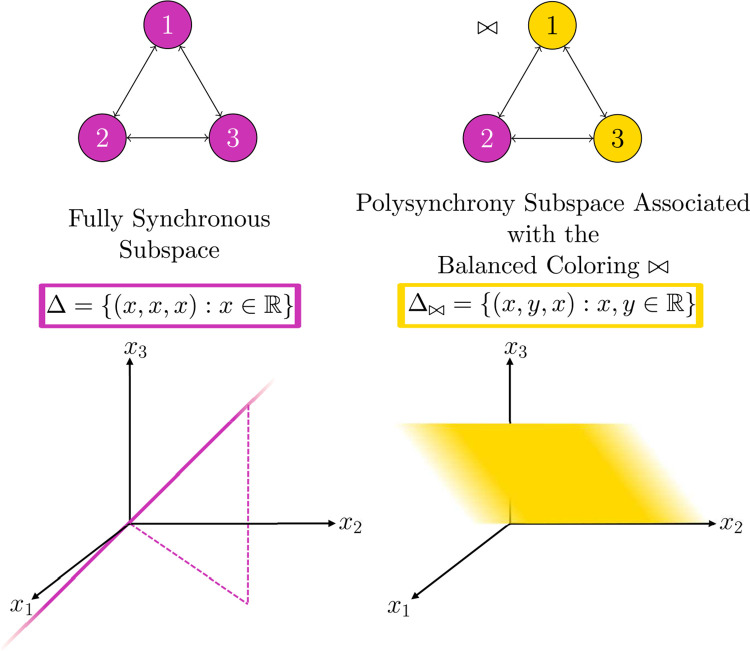 Figure 2
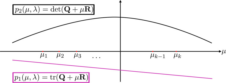 Figure 3
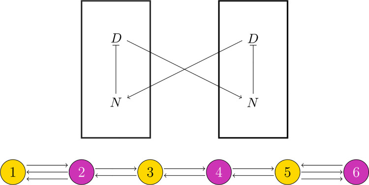 Figure 4
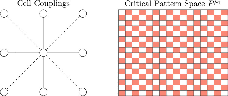 Figure 5
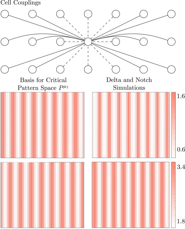 Figure 6
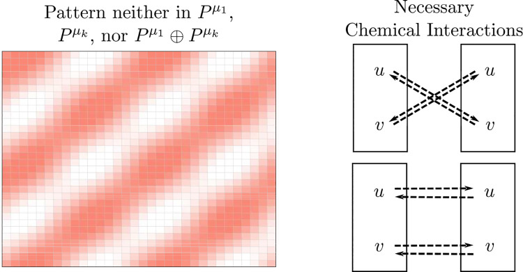 Figure 7
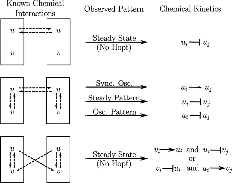 Figure 8
Peer Reviews
No public reviews on file for this paper yet. If you reviewed it on a platform where reviews are public (OpenReview, ICLR, NeurIPS, ICML), you can paste yours below so the community can read it here.
Videos
No videos yet. Explain this paper in a talk, walkthrough, or lecture? Add one.
Taxonomy
TopicsEngineering Applied Research
Introduction
1
Pattern formation is a hallmark of developmental biology, where cells within a tissue or organism differentiate in a precise spatial arrangement to form complex structures. This process is essential for cell fate specification, tissue development, and morphogenesis; and understanding the molecular causes of pattern formation has promising applications in regenerative medicine, tissue engineering, and the treatment of congenital malformations (Chuong and Richardson, 2009).
During development, a group of cells with the same developmental potential will receive a signal called a morphogen that prompts them to communicate and form a pattern of cell types. These local patterning events occur sequentially, with each iteration creating progressively finer cellular patterns across the developing organism. Recent ordinary differential equation (ODE) models have considered one iteration, focusing on how changes in cell-communication and chemical kinetics affect the cellular pattern (Williamson et al., 2021; O’Dea and King, 2012; de Back et al., 2013; Fisher et al., 2005; Irons et al., 2010; Giurumescu et al., 2006; Vasilopoulos and Painter, 2016; Hadjivasiliou et al., 2016). Most models investigate the Notch signaling pathway, which is a key signaling pathway involved in contact-mediated cell-communication. Although the full complexity of the Notch pathway is difficult to model, simplified systems – such as the model from Collier et al. (1996) – have offered valuable insights into how cell-communication can give rise to fine-grained patterns.
Over time, modeling changes have produced further understanding. For instance, O’Dea and King (2012) incorporated morphogens that act as bifurcation parameters, showing how an initially homogeneous steady-state can be destabilized, leading to the formation of patterns. They also derived a continuum model to account for morphogen gradients, showing how tissues with different chemical gradients form different patterns. Williamson et al. (2021) used a similar approach and demonstrated that the structure of communication networks among cells determines the types of fine-grained patterns that can emerge. Others have shown via simulations that coarse-grained patterns such as spots and stripes can arise if there is long-range signaling in the Notch pathway (Vasilopoulos and Painter, 2016; Hadjivasiliou et al., 2016).
Despite the usefulness of these models, they all rely on specific equations; therefore, there are possible dynamics that the models cannot represent due to potentially incomplete assumptions about the system, including assumptions about reaction rates and the molecular pathways involved (e.g. focusing on Notch signaling). Moreover, although model investigation has helped with understanding which parameters are important for pattern formation, the inherent complexity of any model prohibits us from determining which parameters are necessary or sufficient for a pattern. Recent advances in network theory (Golubitsky and Stewart, 2023) allow a more thorough investigation of pattern formation in many cell-communication networks. By ignoring all unnecessary information and focusing on the connectivity of cells (i.e. which cells influence each other), one can predict all possible patterns of cell fates that can emerge in a generic system (Wang and Golubitsky, 2004). Additionally, we provide simple conditions – related to qualitative features of the chemical signaling network – that are both necessary and sufficient for a pattern of cell fates to form under our assumptions.
Using our theory, we find that despite the limited chemical signaling pathways involved in development, cells can generate diverse patterns by reorganizing themselves, thus validating and extending the work of Williamson et al. (2021), Vasilopoulos and Painter (2016), and Hadjivasiliou et al. (2016). On the other hand, cells whose organization is constrained can form various patterns by using different chemical signaling mechanisms, as suggested in de Back et al. (2013). We identify conditions under which cells will fail to form stable patterns, instead remaining in a homogeneous steady-state, oscillating synchronously, or forming oscillating patterns. Importantly, our theory shows that the chemical kinetics proposed in the Collier model are not the only kinetics that can lead to pattern formation. Finally, we are able to infer possible biochemical interactions from an observed pattern, which can reveal previously unknown interactions in biochemical signaling pathways.
The paper is organized as follows. In Section 2, we state our biological assumptions and introduce our mathematical framework, including the theory of network dynamics. We highlight how bifurcations in networks can give rise to patterns corresponding to eigenvectors of the system. In Section 3, we show that qualitative features of chemical signaling determine the stability of the initially homogeneous steady-state and dictate the critical eigenvectors that lead to pattern formation. In Section 3.2, we apply our theory to various biological contexts and predict patterns using minimal modeling assumptions. We show how the same chemical signaling pathway can produce different patterns depending on the cell-communication network. Finally, in Section 3.3, we demonstrate how our framework can be used to infer properties of biochemical signaling pathways from observed patterns in tissues.
Mathematical methods
2
General model assumptions
2.1
We make the following general assumptions to guide the construction of our network models and their associated internal dynamics.
- The cells are well-mixed compartments that can be characterized by the concentration of multiple chemical species inside the cell.
- The concentrations of chemical species within the cells change smoothly over time.
- The cells begin in a nearly identical state.
- The external signals to each cell are identical.
- The cells are in a sufficiently uniform lattice structure. (The lattice may be in 1,2, or 3 spatial dimensions).
- The cells average signals from their neighbors.
Assumptions (1) and (2) allow us to represent our system of cells with ordinary differential equations. Assumptions (3)-(6) allow us to represent our system with a strongly connected, regular network as defined in Section 2.
Network definitions and basic properties
2.2
Our approach emphasizes the role of network structure in pattern formation, so we outline key definitions and properties that will be used throughout the paper (for a fully rigorous treatment, see (Nijholt et al., 2016; Golubitsky and Stewart, 2023)).
Definition 1 (Regular Networks). A regular network is a finite directed graph where
- is the set of nodes
- is the set of arrows
- is the source map
- is the target map.
Additionally, the number of input arrows to each node is the same (i.e. for all ). We call the number of input arrows the valence of the network.
For example, each network shown in Figure 1 (ignoring colors) is a regular network because every node has two input arrows.
There is a class of ODEs called admissible ODEs that is naturally associated with a regular network . Suppose that each node has an associated “state” – where is called the node space. Then the state of an -node network with node space can be described by .
Next, suppose that each node is only influenced by itself and nodes such that there is an arrow from to (i.e. and for some ). Let denote the set of input nodes to (i.e. nodes satisfying and .
Definition 2 (Admissible ODE for a Regular Network). An ODE is called admissible for the regular network if for some smooth function , the dynamics of each node can be written in the form
where the overline indicates that is symmetric in the arguments 2 through .
Definition 3 (Balanced Colorings of Regular Networks). For a regular network , assign every vertex a color via the coloring map
This coloring is balanced if for every with there exists a color-preserving bijection between their input nodes:
Intuitively, a coloring is balanced if for any two nodes with the same color, the set of nodes influencing has exactly the same colors, with the same frequency, as the set of nodes influencing . See Figure 1 for examples of balanced colorings.
Definition 4 (Polysynchrony Subspace). Let be a balanced coloring of a regular network given by the coloring map . The associated polysynchrony subspace is the set
See Figures 1, 2 for examples of balanced coloring and corresponding polysynchrony subspaces.
Definition 5 (Flow Invariance). Let be a smooth vector field. A subspace is flow-invariant under if .
Proposition 1 (Polysynchrony Subspaces are Flow-Invariant). Let be an admissible ODE for the network . Every polysynchrony subspace given by a balanced coloring is flow-invariant under .
The balanced colorings in Figure 1 from left to right correspond to the polysynchrony subspaces
Coloring every node the same is always balanced, and the associated polysynchrony subspace is called the fully synchronous subspace, which we denote . If , we say that the system is fully synchronous.
Eigenvalues depend on cell-level dynamics and network structure
2.3
Consistent with our general assumptions discussed above, we assume that any admissible ODE of a regular network with nodes takes the form
where is a bifurcation parameter.
Let denote the total state of the network, and suppose . If we write the arguments of as
then the internal and coupled dynamics of the system (respectively) are given by
where represents the differential of with respect to the variable . For example,
We remove the arguments of and if it is clear where they are being evaluated.
Definition 6 (Adjacency Matrix). The adjacency matrix of a regular network with n nodes is a matrix with entries defined to be the number of arrows from node to node .
Proposition 2 (Eigenvalues of System via Reduced Matrices). Suppose is a regular network with adjacency matrix and admissible . If are the eigenvalues of (not necessarily distinct) with eigenvectors , and is the Jacobian of at a synchronous equilibrium , then the eigenvalues of are the union of the eigenvalues of where and are the internal and coupled dynamics, respectively. Furthermore, the corresponding eigenvectors are where is an eigenvector of .
Proof. See (Golubitsky and Stewart, 2023).
The critical eigenvalue dictates the preferred pattern
2.4
We assume that pattern formation occurs from a synchrony-breaking bifurcation and argue the first bifurcating pattern is the “preferred” pattern of a tissue. When the homogeneous steady-state is destabilized via a bifurcation, the critical eigenvalue corresponds to a pattern (Theorem 3), which is generically the only stable bifurcating pattern (Proposition 4). We assume that the bifurcation parameter changes much slower than the state of the cells. With a quasistatically (slowly) varying , the uniform state can lose stability with a stable patterned state emerging; thus, the system will move from the homogeneous state to the pattern state and will remain there unless there is a secondary bifurcation on the pattern branch. Furthermore, as in Poston and Stewart (1978), we may assume that the only bifurcations present are those that are forced by our assumptions and observed data. Extraneous secondary bifurcations would violate Occam’s Razor – the principle that the simplest model which can explain observed phenomena is best. Even with secondary bifurcations, the preferred pattern is the only stable pattern for some region of the parameter space, and it is reasonable that unusual behaviors can arise for unrealistic parameter values.
Theorem 3 (Patterns Bifurcating from Synchrony). Let be a regular network with admissible . Let denote the fully synchronous subspace, and let be the polysynchrony subspace associated with the balanced coloring . Assume that there is a synchronous equilibrium and that has a critical eigenvalue . Denote the associated generalized eigenspace . If and , then generically a unique branch of equilibria with synchrony pattern bifurcates from at .
Proof (modified from (Golubitsky and Stewart, 2023)). Since is nonsingular. Thus, by the implicit function theorem, there exists a synchronous branch of equilibria in the neighborhood of . By a change of coordinates, we can assume that the synchronous branch is given by . Since , the kernel of is 1-dimensional, so we can use Liapunov-Schmidt reduction to find a reduced equation of the restriction given by
for some vectors . The zeros of are in one-to-one correspondence with the zeros of in a neighborhood of the bifurcation.
Since the spatial domain and codomain of are 1-dimensional, we can write
for and . Liapunov-Schmidt can be chosen to preserve the existence of the trivial solution, so we may assume .
The eigenvalue crossing condition and reduction imply that is generically nonzero. Thus, by the implicit function theorem for some function of . Since we can write as a function of in a neighborhood of the bifurcation, there exists a branch of solutions to and thus to . □
Proposition 4 (Subsequent Branches are Unstable). Suppose is a regular network with admissible . Let be the adjacency matrix with eigenvalues , and assume there exists a synchronous branch of equilibria that is stable for (for some ). Suppose that has a critical eigenvalue that is an eigenvalue of the matrix . Furthermore, suppose that for has no critical eigenvalues that are eigenvalues of . If there is a bifurcation at with critical eigenvalue from for , then generically the bifurcating branches are unstable.
Proof. We initially assume that the synchronous equilibrium is stable. If there is a bifurcation at with a critical eigenvalue of , the synchronous equilibrium will generically lose stability. In particular, there will be a positive eigenvalue that is an eigenvalue of . If there are no critical eigenvalues of for , then will remain positive at the bifurcation point . Since the eigenvalues of the Jacobian continuously depend on ( ), the bifurcating branches will be unstable in some neighborhood of the bifurcation point. □
Other preliminaries
2.5
For our results, we will use the definition of a strongly connected graph and the well-known Perron-Frobenius theorem.
Definition 7 (Strongly Connected Network). A network is called strongly connected if for every pair of nodes with , there is a path from to and from to .
Theorem 5 (Perron-Frobenius). If a network is strongly connected, then the adjacency matrix has a simple positive eigenvalue equal to the spectral radius . For all other eigenvalues *of *, .
Proof. See (Golubitsky and Stewart, 2023).
Results
3
The internal and coupled dynamics determine the preferred pattern
3.1
The adjacency matrix of the cell-communication network determines the possible patterns that can form in the tissue. Qualitative features of the internal and coupled dynamics select the preferred pattern from all possible ones.
We assume that is a strongly connected regular network on nodes without self-arrows (i.e. for any there is no with and ). Denote the adjacency matrix . We consider an arbitrary admissible ODE with a synchronous branch of equilibria that is stable for . We assume that the Jacobian of the ODE is singular at . Lastly, we take and to be the linearized internal and coupled dynamics (respectively), which are defined whenever (Section 2.3).
Definition 8 (Critical Pattern Space). Suppose that has distinct eigenvalues and corresponding eigenvectors . Let be given by
Suppose that has critical eigenvalues that by Proposition 2 are null eigenvalues of for some . Then define the critical pattern space to be the subspace of given by
Proposition 6 (Stability of Synchronous 1-Dimensional Nodes). If the node space is 1-dimensional and the synchronous equilibrium is stable, then .
Lemma 6.1. The adjacency matrix always has a strictly positive eigenvalue and an eigenvalue with strictly negative real part.
Proof of lemma. The adjacency matrix of a regular graph always has a unique largest eigenvalue equal to its valence (see Definition 1). Furthermore, since we assume our graph has no self-arrows, every element on the diagonal of is zero, and . Since the trace is the sum of the eigenvalues and there exists a positive eigenvalue, there must be some eigenvalues with negative real part. In particular, the eigenvalue with smallest real part, which we denote , has negative real part. □
Proof of proposition. Recall that the eigenvalues of the system are where are the eigenvalues of the adjacency matrix (Proposition 2). By Lemma 6.1, has a positive eigenvalue and an eigenvalue with negative real part. Let each eigenvalue be written
where . For the remainder of this proof, we will drop the arguments of the internal and coupled dynamics, and (respectively), writing
Since is stable, the real part of each eigenvalue for all . By Lemma 6.1, we can choose such that . Then
□
Proposition 7 (Stability of Synchronous 2-dimensional Nodes). Let the node space be 2-dimensional, and suppose that has distinct real eigenvalues , not counting multiplicity. If the synchronous branch is stable, then .
Proof. Since is stable,
for . By Lemma 6.1, there exists positive and negative eigenvalues of . Let be an eigenvalue with the same sign as . Then
□
Lemma 7.1. Suppose that is a polynomial in smoothly parameterized by . Let be a set of points in . Let , and suppose that for all we have for all . Suppose that at is linear in and there exists some such that . Then we have the following cases
for all if and only if . and if and only if . and if and only if .
Proof. For the forward direction of (1), if for all , then since it is a linear function of ; therefore, . For the converse, suppose that . Then . By hypothesis, there exists some such that . Clearly, this implies that . Thus, , so for all .
For the forward direction of (2), suppose that and for all . This implies that for any ,
Equivalently,
Since , we must have that .
For the converse, suppose that . If
then since ,
but this contradicts the continuity of with respect to since for . Hence, must be the unique point from with .
For the forward direction of (3), suppose that and for all . This implies that for any ,
Equivalently,
Since , we must have that .
For the converse, suppose that . If
then since ,
but this contradicts the continuity of with respect to since for . Hence, must be the unique point from with . □
Theorem 8 (Characterizing the First Branch in 1-Dimension). Let have eigenvalues ordered by real part, and assume that the node space is 1-dimensional. Then we have the following mutually exclusive cases
The critical pattern space is if and only if .The critical pattern space is , and the bifurcation is synchrony-breaking if and only if .The critical pattern space is (a vector of ones of length ), and the bifurcation is synchrony-preserving if and only if .
Proof. Let be the eigenvalues of with distinct real parts . Take to be the linear polynomial in given by
so that gives the real part of some eigenvalue of . Since we assume that the synchronous branch is stable before the bifurcation, there exists such that for all for all . Furthermore, at the bifurcation point, there exists some with . Therefore, the hypotheses of Lemma 7.1 are satisfied.
Applying Lemma 7.1, we have the following three cases.
- for all if and only if .
- and if and only if .
- and if and only if .
exactly when the system has the critical eigenvalue . Using Definition 8 the main conclusion immediately follows.
Lastly, the unique eigenvalue of with largest real part is the unique eigenvalue with eigenvector (a vector of ones). By Proposition 2 and Theorem 3, the bifurcation with critical eigenvalue is synchrony-preserving, whereas bifurcations with other critical eigenvalues are generically synchrony-breaking. □
Theorem 9 (Characterization of Bifurcations in 2-dimensions with ). Suppose that the node space is 2-dimensional and the adjacency matrix has real eigenvalues , where each has algebraic multiplicity and geometric multiplicity . Suppose that , and take
In Table 1, we enumerate all possible critical pattern spaces, the multiplicity and type of critical eigenvalues, and the dimension of the critical eigenspaces. For the first four cases listed, we give necessary and sufficient conditions on the internal and coupled dynamics for such a bifurcation to occur. For the remaining cases, we give necessary conditions, which are sufficient if we assume the bifurcation is sufficiently degenerate.
Proof. We want to use the trace and determinant to obtain information about the eigenvalues; therefore, define the following polynomials of :
We will drop the argument if it is obvious where the polynomial is being evaluated. Since we assume that , we have that
We also assume the synchronous equilibrium is initially stable, so there exists such that for all ,
for all . This setup is illustrated in Figure 3. For a bifurcation to happen, there exists such that either or (or both). Applying lemma 3.1.2 (to and ), we have that
- and if and only if .
- and if and only if .
- and if and only if .
- and if and only if .
- for all if and only if .
- for all if and only if .
Now, let’s consider some of the possible cases. Notice that by equations (1) and (2) and the continuity of both polynomials with respect to , if , then we must have . Similarly, if , then we must have .
If and , there are complex conjugate pairs critical eigenvalues that are eigenvalues of ; if and , then there are real critical eigenvalues that are an eigenvalue of ; and if , there are real critical eigenvalues that are the two eigenvalues of with multiplicity .
Lastly, by the Perron-Frobenius Theorem, . We use this information to enumerate all possibilities in Table 1. □
Theorem 10 (Nondegeneracy Conditions in 2-Dimensions). Assume that has valence . Suppose that the node space is 2-dimensional and the adjacency matrix has distinct real eigenvalues and corresponding algebraic multiplicities . Suppose that and take
- Suppose that at where denotes the logical “or.” If
then the critical eigenvalues are the pair of imaginary eigenvalues from a single matrix , with multiplicity . 2. Suppose that at . If
then the critical eigenvalues are a real eigenvalue from a single matrix with multiplicity .
Proof. Since we can obtain important information about the eigenvalues of a 2×2 matrix using the trace and determinant, define the following polynomials of :
Again, this setup is illustrated in Figure 3. We will drop the arguments if it is obvious where the polynomial is being evaluated. Since we assume that , we have that
Suppose that at the bifurcation. Of course, this implies that . Furthermore, by the Perron-Frobenius theorem is the spectral radius of (i.e. the largest absolute value of its eigenvalues). Therefore, for any ,
and
Since for all , the critical eigenvalues must correspond to pairs of imaginary eigenvalues, given by matrices such that . In the case that , there is exactly one root of the line , implying that at the bifurcation, there is a unique such that . Thus, there is a pair of imaginary critical eigenvalues that are eigenvalues of . Since is an eigenvalue of with multiplicity , the critical eigenvalue is an eigenvalue of with multiplicity . Now, notice that implies (otherwise the synchronous branch would be unstable before the bifurcation), and thus our analysis of the case that reduces to the previous case that .
For (2), suppose that at the bifurcation. Then . Furthermore, for any ,
and
Since for all at the bifurcation, any critical eigenvalues must be real and given by matrices with . Using the same logic as previously, if , there can be exactly one root of the line , implying that at the bifurcation there is a unique with , giving a real critical eigenvalue that is an eigenvalue of . Since is an eigenvalue of with multiplicity , the critical eigenvalue is an eigenvalue of with multiplicity . We also have that implies that (otherwise the synchronous branch would be unstable before the bifurcation), thus reducing to the prior case. In both cases, since and the critical eigenvalue is real. □
We have shown that for a 2-dimensional node space, if – as is the case for Notch signaling (Section 3.2.1) – then any stable pattern that forms generically corresponds to the critical pattern space . If , however, then a stable pattern can correspond to any critical pattern space as shown below. This indicates two possible mechanisms for the diversity of patterns we see in biological systems: cells reuse chemical signaling pathways but reorganize themselves to change communication, or cells use different chemical signaling pathways.
Theorem 11 (Existence of Admissible ODE for Arbitrary First Branch, Golubitsky and Stewart). Suppose the adjacency matrix has distinct real eigenvalues . Then for any , there exists an admissible system with 2-dimensional node space such that the critical pattern space is .
Proof. See (Golubitsky and Stewart, 2023).
Theorem 12 (Sufficient Condition for Pattern in or ). Suppose that the node space is 2-dimensional and the adjacency matrix has distinct real eigenvalues not counting multiplicity. If , then the critical pattern space is either , or .
Proof. As before, let
If or , then there are critical eigenvalues from for all , and the critical pattern space is .
Now suppose that and . Then, there is a critical eigenvalue that is an eigenvalue of if and only if either or . From Lemma 7.1, if then .
is a quadratic polynomial in whose graph is downward opening (Figure 3), so its derivative is linear with slope 2 . Suppose that for for contradiction. We have two cases:
- If , then since . But this contradicts the continuity of in since for , otherwise the branch would not be stable.
- Similarly, if , then since , which again contradicts the continuity of as a function of . □
In conclusion, since or can only occur for or , there can only be critical eigenvalues from or (or both), which gives us our conclusion by Proposition 2 and Definition 8.
Predicting patterns from qualitative features of cell-communication and chemical kinetics
3.2
We use theorems in Section 3.1 to predict patterns of cell fates given qualitative features of Notch signaling and the cell-communication network.
Critical pattern space of Notch signaling is Pμ1
3.2.1
Following the model of Collier et al. (1996), the feedback between Delta and Notch in coupled cells can be represented as in Figure 4 (top) where Notch inhibits Delta within a cell and Delta activates Notch in neighboring cells. It is natural to assume that activates (represented with ) means that
and inhibits (represented with ) means that
Furthermore, we assume that Delta and Notch both decay over time, meaning that
Writing the concentrations of the biochemical species as a vector , the internal and coupled dynamics of the Delta-Notch signaling pathway take the form
where + denotes a positive term, and – denotes a negative term. Thus, we have ; if has real eigenvalues, we can apply Theorem 9.
We also have that
so from Table 1, the critical pattern space is .
Preferred pattern in mutated C. elegans vulval precursor cells (VPCs)
3.2.2
The C. elegans vulval precursor cells (VPCs) form a pattern that is mediated by Notch signaling. With a mutation of let-23, all VPCs receive approximately equal external signals (Aroian and Sternberg, 1991), so the system can be represented with the regular network in Figure 4 (bottom). The adjacency matrix is
Using Matlab, we find that the eigenvalues are real, and the smallest eigenvalue and its corresponding eigenvector are
implying that the critical pattern space has geometric multiplicity 1, so the critical eigenspace is 1-dimensional (Table 1), and the critical pattern space corresponds to the balanced coloring shown in Figure 4 (bottom), so Theorem 3 implies that there is a bifurcating branch of solutions with the pattern . Furthermore, Proposition 4 implies that this will generically be the only stable branch, so we expect the C. elegans vulva, with a mutation of let-23, to exhibit an alternating pattern of cell fates – and this is exactly what is observed experimentally.
Preferred patterns in square arrays of cells developing according to Notch signaling
3.2.3
We will compute the critical pattern space of two square arrays of cells that develop according to Notch signaling (Figures 5,6), showing that cells can change their communication to form a different pattern despite using the same signaling mechanism.
We have shown that the critical pattern space for the Notch pathway is , so we must compute to determine the preferred pattern of the tissue. depends on the cell-communication network. In Figure 5, we consider a 16 × 16 array of cells, where each cell is coupled to its neighbors as depicted on the left (for clarity, we omit arrows pointing towards the central cell), and there are periodic boundary conditions. Dotted lines represent a connection strength of 1, and solid lines represent a connection strength of 3. Since there are periodic boundary conditions, the adjacency matrix will be real and symmetric, so will have real eigenvalues. Using Matlab, we find that the smallest eigenvalue gives the checkerboard pattern on the top-right, which matches our simulations.
In Figure 6, we consider a 50 × 50 array of cells with couplings shown in the top panel and periodic boundary conditions. Using Matlab, the minimal eigenvalue has geometric multiplicity 2, and the critical pattern space is the 2-dimensional space spanned by the vectors depicted on the left of Figure 6. In Table 1, , and we do not attempt to show that for some coloring , so the hypotheses of Theorem 3 may fail. Thus, we cannot ensure that there is a solution with the pattern of the critical pattern space; however, our numerical simulations validate that the predicted pattern is realized for some parameter range, as shown on the right of Figure 6.
Inferring biochemical interactions from observed patterns
3.3
Finally, we show how the theory can be used to infer properties of the chemical signaling pathway from an observed pattern.
For a 16 × 16 array of cells communicating as in Figure 5 (left), if we observe the striped pattern in Figure 7 (left), then the critical pattern is neither , nor . Barring the extremely degenerate case that the critical pattern space is , we must have that (Theorem 12), so the development is due to a chemical signaling network with the connections given on the right of Figure 7 (top or bottom).
Now, suppose there is some regular array of uniform cells. If we have partial information about chemical signaling in a tissue, we can use the observed tissue pattern to obtain additional information about chemical signaling by using the following steps.
- Use the partial information about chemical interactions to create matrices representing the internal dynamics and coupled dynamics with variables as entries.
- Use Theorems 6 and 7 to determine the signs of several variables in and .
- Check . Then reference the observed pattern against Table 1 to determine necessary conditions on and .
- Use newfound information about and to determine the possible signs of additional variables in and .
- Lastly, convert the information about the sign of entries in and to information about activation and inhibition of biochemical species.
For the first example, consider when one chemical in a cell influences the same chemical in a neighboring cell, and suppose that the chemical is independent of other chemical species. Then the node space is 1-dimensional, and we can represent the internal and coupled dynamics as in Figure 8 (top). This tells us that
For the uniform or synchronous state to be stable, we must have that (Proposition 6), implying that decays. Assume that decays at the same rate for all time. Then for a pattern to form, there must be a synchrony-breaking bifurcation, which by Theorem 8 occurs if and only if , meaning that in one cell must inhibit in its neighboring cells, and the inhibition must increase for a synchrony-breaking bifurcation to occur.
Now, suppose we know that the concentration of is affected by the concentration of another chemical within the cell (Figure 8, middle). Then writing the chemical species as a vector ,
for some real numbers .
If the cells are initially uniform, then from Proposition 7,
This is satisfied if both chemical species decay – as is standard. Furthermore, notice that
so we can apply Theorem 9. If the cells oscillate in sync, then we may assume that there was a synchrony-preserving Hopf bifurcation, implying that (Table 1, row 4), so . If they oscillate in a pattern, then we may assume there was a synchrony-breaking Hopf bifurcation, implying that (Table 1, row 2) and thus . If we see that a steady-state pattern has formed among the cells, then we can infer that a synchrony-breaking steady-state bifurcation occurred (Table 1, row 1) meaning that
Assuming that decays, , implying that and the strength of decay of or the strength of inhibition must increase for a pattern to form.
Lastly, assume that in cell influences in neighboring cells as shown by the general diagram in Figure 8 (bottom). Writing the chemical species as a vector , we have that the internal and coupled dynamics are given by
for real numbers .
If the cells are initially uniform, then from Proposition 7,
Again, this is satisfied if both chemical species decay. Furthermore, notice that
so applying Theorem 9, we are in the first or third row of Table 1. This means there can only be a steady-state bifurcation (i.e. no oscillatory behavior). And
If , then synchrony cannot be broken since (see Table 1). If we observe a pattern, however, then we expect that , meaning that we either have
- and
- or and .
Discussion
4
This framework provides powerful tools for molecular biologists who are interested in uncovering the mechanisms of pattern formation. It provides a systematic approach to identifying the molecular causes of pattern failures, which can help guide protein knockdown experiments in model organisms. Additionally, our theory can help uncover unknown molecular interactions in chemical signaling networks through the analysis of patterns that emerge in tissues (Figure 8).
This framework was created by recognizing that a developing tissue can be modeled as a system of ODEs on a regular network. When the linearization has null eigenvalues, a pattern can form through a bifurcation (Theorem 3). Using the network framework, we can determine the eigenvalues by examining smaller matrices , where represents an eigenvalue of the adjacency matrix , while and represent the linearized internal and coupled dynamics, respectively (Proposition 2). Thus, the pattern is determined by both the global cell-communication structure and the local cell-level dynamics ( and ).
We use our assumptions about a developing tissue to gain information about the pattern and chemical kinetics. Since the synchronous state is initially stable, all eigenvalues are negative, which provides crucial information about the chemical kinetics described by and (Propositions 6, 7). Then for a pattern to form, must have a null eigenvalue for some . We found that in nondegenerate systems with either one or two biochemicals and one coupling between cells, the resulting steady-state pattern always corresponds to the smallest eigenvalue of (denoted ) and is given by the critical pattern space (Definition 8). The formation of the pattern, however, requires specific conditions on and (Theorems 8, 9).
Altogether, our theory suggests that (1) if the chemical kinetics and satisfy certain conditions, then a pattern will form that is dictated by the cell-communication structure (Section 3.2); and (2) if a pattern forms in an array with known communication structure , then the chemical kinetics and must satisfy certain properties (Section 3.3).
Our framework also extends beyond basic research with several potential applications. In tissue engineering, our findings suggest that controlling the range of cell-communication can guide pattern formation (Section 3.2.3). Alternatively, maintaining the same communication structure while adjusting chemical signaling can alter the tissue pattern (Figure 7). In medicine, these insights have important implications for understanding disease mechanisms, as disruptions in pattern formation are associated with congenital malformations. We provide a theoretical framework for understanding the molecular changes underlying these failures. In particular, our theory illustrates that multiple molecular factors can lead to the same pattern breakdown. This helps explain why drugs can treat a disease for some individuals but not others and suggests novel drug targets.
Although our framework relies on simplified assumptions about biological systems, future research will refine and expand its applicability. A key next step will be extending our analysis from two-dimensional signaling networks to more complex, realistic biochemical systems. This expansion will improve our ability to identify the molecular causes of pattern formation. Additionally, we plan to validate our theoretical predictions through simulations that incorporate spatial features including morphogen gradients, parameter noise, and network perturbations, enabling us to apply our theory to a broader range of biological contexts.
The reference list from the paper itself. Each links out to its DOI / PubMed record.
- 1Aroian R.V., Sternberg P.W.: Multiple functions of let-23, a caenorhabditis elegans receptor tyrosine kinase gene required for vulval induction. Genetics 128(2), 251–267 (1991)2071015 10.1093/genetics/128.2.251PMC 1204464 · doi ↗ · pubmed ↗
- 2Collier J.R., Monk N.A., Maini P.K., Lewis J.H.: Pattern formation by lateral inhibition with feedback: a mathematical model of delta-notch intercellular signalling. Journal of theoretical Biology 183(4), 429–446 (1996)9015458 10.1006/jtbi.1996.0233 · doi ↗ · pubmed ↗
- 3Chuong C.-M., Richardson M.K.: Pattern formation today. The International journal of developmental biology 53(5–6), 653 (2009)19557673 10.1387/ijdb.082594 cc PMC 2874132 · doi ↗ · pubmed ↗
- 4Back W., Zhou J.X., Brusch L.: On the role of lateral stabilization during early patterning in the pancreas. Journal of The Royal Society Interface 10(79), 20120766 (2013)23193107 10.1098/rsif.2012.0766 PMC 3565694 · doi ↗ · pubmed ↗
- 5Fisher J., Piterman N., Hubbard E.J.A., Stern M.J., Harel D.: Computational insights into caenorhabditis elegans vulval development. Proceedings of the National Academy of Sciences 102(6), 1951–1956 (2005)10.1073/pnas.0409433102 PMC 54855115684055 · doi ↗ · pubmed ↗
- 6Golubitsky M., Stewart I.: Dynamics and Bifurcation in Networks: Theory and Applications of Coupled Differential Equations. Society for Industrial and Applied Mathematics, Philadelphia, PA (2023). 10.1137/1.9781611977332. https://epubs.siam.org/doi/abs/10.1137/1.9781611977332 · doi ↗
- 7Giurumescu C.A., Sternberg P.W., Asthagiri A.R.: Intercellular coupling amplifies fate segregation during caenorhabditis elegans vulval development. Proceedings of the National Academy of Sciences 103(5), 1331–1336 (2006)10.1073/pnas.0506476103 PMC 136052416432231 · doi ↗ · pubmed ↗
- 8Hadjivasiliou Z., Hunter G.L., Baum B.: A new mechanism for spatial pattern formation via lateral and protrusionmediated lateral signalling. Journal of the Royal Society Interface 13 (2016) 10.1098/rsif.2016.0484 PMC 513400927807273 · doi ↗ · pubmed ↗