Modeling approaches for assessing device-based measures of energy expenditure in school-based studies of body weight status
Gilson D. Honvoh, Roger S. Zoh, Anand Gupta, Mark E. Benden, Carmen D. Tekwe

TL;DR
This paper explores how wearable devices can track energy expenditure in schools to better understand how physical activity affects children's BMI.
Contribution
The study introduces advanced statistical models to analyze energy expenditure patterns and their impact on BMI across different quantiles.
Findings
Functional quantile mixed-effects models (FQMEM) show significant associations between energy expenditure and BMI for short time intervals.
Quantile models reveal that white students have lower BMI at specific quantiles compared to non-white students.
Functional models allow for assessing the influence of physical activity timing on BMI, which traditional models cannot.
Abstract
Obesity has become an important threat to children’s health, with physical and psychological impacts that extend into adulthood. Limited physical activity and sedentary behavior are associated with increased obesity risk. Because children spend approximately 6 h each day in school, researchers increasingly study how obesity is influenced by school-day physical activity and energy expenditure (EE) patterns among school-aged children by using wearable devices that collect data at frequent intervals and generate complex, high-dimensional data. Although clinicians typically define obesity in children as having an age-and sex-adjusted body mass index (BMI) value in the high percentiles, the relationships between school-based physical activity interventions and BMI are analyzed using traditional linear regression models, which are designed to assess the effects of interventions among children…
Genes, proteins, chemicals, diseases, species, mutations and cell lines named across the full text — each resolved to its canonical identifier and authoritative record.
Click any figure to enlarge with its caption.
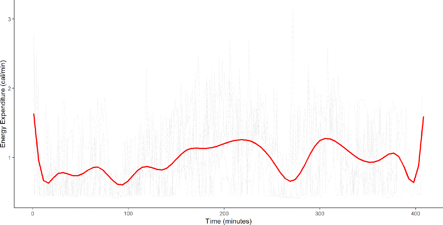 Figure 1
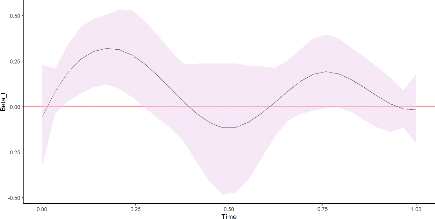 Figure 2
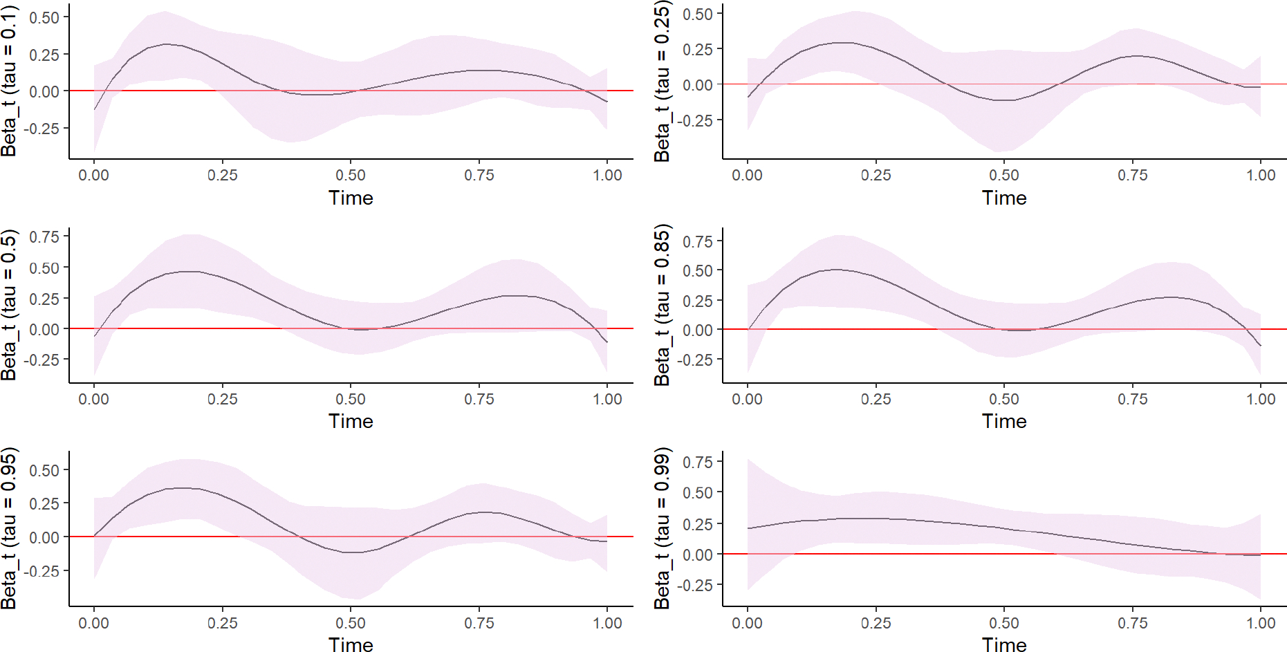 Figure 3
Peer Reviews
No public reviews on file for this paper yet. If you reviewed it on a platform where reviews are public (OpenReview, ICLR, NeurIPS, ICML), you can paste yours below so the community can read it here.
Videos
No videos yet. Explain this paper in a talk, walkthrough, or lecture? Add one.
Taxonomy
TopicsObesity, Physical Activity, Diet · Body Composition Measurement Techniques · Solar Radiation and Photovoltaics
Introduction
1
Approximately 90% of children diagnosed with type 2 diabetes are classified as either overweight or obese (1). Obesity has been linked to various factors, including a chronic imbalance between energy expenditure (EE) and energy intake, environmental exposures, and genetic predispositions. However, the exact contributions of EE to obesity development remain unclear (2). To combat the growing obesity epidemic among children, behavioral researchers increasingly employ targeted, school-based interventions designed to reduce school-day sedentary behaviors among children (3–5). The effects of these interventions on physical activity (PA) are often monitored using wearable devices, such as accelerometers, which collect frequent measures of estimated calorie expenditures or the number of steps taken (6, 7). Wearable devices typically record data at either the second or minute level over multiple days to monitor PA intensity. Often, these measures are used to estimate the metabolic equivalent of tasks, which can be used to derive the amount of time spent performing sedentary, light, moderate, or vigorous PA (8). Alternatively, the data collected over time by wearable devices can be represented by scalar-valued summary numbers such as mean EE or total EE, or by curves (9–12). When data are presented as curves, functional data analysis, which treats curves as the unit of statistical analysis, is a modeling strategy (13–15). Functional data analysis applies data reductions techniques to the curves and subsequently uses regression approaches for statistical modeling. The data reductions can simply consist in summarizing the data from minute-level observations into hourly mean EE values (11). Furthermore, more complex statistical data reduction techniques, such as functional principal components analyses or polynomial basis expansions, have also been used to for approximating the mean of the curves data have also been used (9, 10, 13, 16–19). Polynomial basis expansions approximate curves by describing their shapes using a few key features, summarizing the information contained within curves into basis functions that adequately capture patterns. Unlike summary statistics, such as the mean, which account for only one source of variation in the data, each basis function accounts for a different source of variation (10). Parametric regression approaches, such as nonlinear or polynomial mixed-effects models, have been considered in functional data settings to parametrically model the effects of curves on an outcome (20–22); however, these approaches are limited by the requirement for strong assumptions regarding the shape of the curve. Thus, semiparametric and nonparametric approaches, which provide more flexibility for fitting curves to data by not requiring a specific parametric form, are standard approaches for analyzing functional data (23–25). Additionally, the ability of these approaches to easily accommodate the high dimensionality of functional data is desirable (13, 14).
In children, overweight and obesity are defined according to age-and sex-adjusted body mass index (BMI) values in the upper ranges (26, 27). However, most studies assessing the impacts of behavioral interventions on BMI rely on traditional linear regression models, which are designed to assess the effects of intervention among children within the normal BMI range and have limited ability to assess the effects of interventions among children classified as overweight or obese. Thus, statistical approaches that permit the evaluation of covariate effects across the entire BMI distribution are preferable when assessing the effects of interventions among children classified as overweight or obese (28). Quantile regression is a statistical technique used to estimate the effects of predictors on quantile functions of a response variable (28–33), such as the median (50th), 85th, or 95th quantiles. Quantile regression is advantageous compared with linear regression because quantile regression does not require the regression residuals to be normally distributed. Using classical mean regression models, such as linear regression, to model BMI as an outcome can provide incomplete information regarding BMI values that lie beyond the mean value, such as values within the distribution tails. Additionally, covariates such as PA and age may have differential impacts on different quantile levels. Therefore, statistical approaches that allow covariate effects to be assessed across the full spectrum of quantile functions are preferable when using BMI as an outcome in obesity studies (28, 29).
Different approaches have been used for assessing the relationship between device-based measures of PA patterns and BMI. Wendel et al. (34) recently used classical linear regression to analyze the effects of introducing stand-biased desks in school on the average change in BMI. Their results indicated that compared with using conventional desks, using stand-biased desks significantly reduced the average change in BMI (p = 0.04). However, analyzing the average change in BMI does not allow for the assessment of how standing desk use affects values above or below the average BMI change. Benden et al. (3) reported that children who used stand-biased desks had a significantly higher mean EE (estimate [Est.] = 0.16, standard error [SE] = 0.04, p < 0.001) than students who used traditional desks. Benden et al. used a hierarchical LMEM to assess the impacts of standing desk use on average SDEE (as a measure of PA); however, this approach is limited to assessing the impacts of standing desk use for those children with “average” SDEE values and cannot assess impacts for those children with SDEE values above or below the average. Additionally, the hierarchical LMEM employed did not model SDEE data as curves.
Trinh et al. (35) studied the effects of PA patterns at baseline on the 3-year change in BMI among elementary school–aged children in Australia and found little evidence to indicate that baseline PA patterns were predictive of future obesity risk when applying classical regression methods that treated objective measures of PA as a summary statistic (average step count per minute) (35). However, using summary statistics to describe PA intensity does not account for potential diurnal PA patterns (9, 11, 12, 36, 37). Approaches that allow assessments of diurnal patterns in PA have also been considered in the literature. For example, Tekwe et al. (9) used functional principal components methods and scalar-on-function regression to analyze EE data (38). These approaches allowed the impacts of diurnal PA patterns on obesity-related outcomes to be assessed. Augustin et al. (12) also considered semiparametric approaches to describe PA patterns and used a histogram of the PA distribution as a predictor in their regression model. Using data from the Avon Longitudinal Study of Parents and Children, Augustin et al. established that their approach provided better fits than summary statistics–based methods.
Our current work was motivated by the stand-biased desk study in which a school-based PA intervention study was assessed (3). The cluster-randomized study was conducted from 2011 to 2013 in three elementary schools within the College Station Independent School District (CSISD) (3). The study is described in detail elsewhere (3); briefly, at the beginning of the 2011–2012 academic year, 24 teachers from three elementary schools were recruited and randomly assigned to the use of either stand-biased desks with stools [Stand2learn LLC College Station, TX, USA, stand-biased desk (model S2LK04) and stool (model S2LS04)] or traditional desks (model 2200 FBBK Series by Scholar Craft Products, Birmingham, AL) with chairs (9000 Classic Series, by Virco Inc., Torrance, CA, USA) for in-class activities (3). A total of 374 students in second through fourth grades were included in the study at baseline. To calculate BMI, each student’s height and weight were measured at the start of each semester by trained research assistants. Study participants were required to wear calibrated BodyMedia SenseWear^®^ armband devices (BodyMedia, Pittsburgh, PA) during school hours for 1 school week in each semester from Fall 2011 to Spring 2013. The devices recorded subject-specific step counts and caloric EE per minute while worn. All study participants consented or assented to participate in the study, and consent to participate was obtained from the parents or legal guardians of all participants. The study protocol was approved by the Institutional Review Board, Human Subjects Program at Texas A&M and the CSISD Review Board.
Using a hierarchical linear mixed effects model, Benden et al. (3) showed that children in stand-biased desk classrooms had significantly higher EE than children in traditional desk classrooms (estimate [Est.] = 0.16, standard error [SE] = 0.04, p < 0.001) in the Fall semester, after adjusting for grade, race and gender. However, using a summary value in the hierarchical linear mixed model does not take advantage of the high dimensionality of EE. Figure 1 illustrates such high dimensionality by showing EE data gathered every minute over 5 school days for a randomly selected student participant in our motivating stand-biased desk study. Nonparametric smoothing was used to approximate the average EE recorded over the five school days for a randomly selected student. By smoothing the mean, we uncover underlying patterns in the data while retaining important features (20, 39). The hierarchical linear mixed model does not provide the ability to assess the impact of these underlying patterns on childhood obesity, thus limiting interpretability.
In this manuscript, we use different modeling approaches to examine the relationship between PA and body weight status, as indicated by measures of BMI. We describe the use of a linear mixed-effects model (LMEM), a quantile mixed-effects model (QMEM), a functional mixed-effects model (FMEM), and a functional quantile mixed-effects model (FQMEM) to study the relationship between school-day EE (SDEE) and BMI. We include random effects in all models to account for clustering and treat SDEE as both a scalar-valued summary and a function-valued predictor variable. We discuss the advantages and disadvantages of each modeling approach. The manuscript is organized as follows. In Section 2, we describe the statistical models employed in our applications. The results from our analyses are provided in Section 3, and we offer some concluding remarks in Sections 4 and 5.
Model specifications
2
In this manuscript, we analyzed data collected at baseline (Fall 2011). Our analytic sample of 256 participants excluded those with large proportions of missing or incomplete accelerometer data. Mean hourly SDEE values were obtained by calculating hourly averages of minute-level device-measured observations across the 5 days of a school week during which the devices were worn. In our analytic sample, all students had exactly 30 mean hourly SDEE values. For all models, we used log (BMI), the natural logarithm of BMI as the response variable and we adjusted for the following covariates: age, sex (boys vs. girls), and intervention (stand-biased desks vs. traditional desks). Given the cluster-randomized design, we attempted to account for the clustering effects of teachers within schools. However, due to computational and convergence issues, we only included a random intercept for schools in all models. We implemented linear regression and quantile regression models with the R software packages lme4 (40) and lqmm (41, 42), respectively. Below, we provide descriptions of the different models considered.
In the remaining of this section, we provide descriptions of the models considered.
Linear mixed-effects model
2.1
Mixed effects models are used to account for clustering in regression models (43). The following model was specified for the LMEM used for students clustered within schools.
In this model, represents the response for the th subject within the th school, is a scalar-valued intercept, and represents the coefficient on the th covariate (overall mean SDEE, age, sex, race, and intervention). For SDEE, we obtained the overall mean of the high-dimensional data recorded for each student. We included the random intercept to account for clustering within schools, and represented the model error associated with . We assume that and . Random effects and errors terms are commonly assumed to be normally distributed based on large sample theory, and also for mathematical and computational convenience.
Quantile mixed-effects model
2.2
The quantile mixed effects model accounts for clustering with random effects in the linear conditional quantile functions (42). We applied the QMEM at the 10th, 25th, 50th, 85th, 95th, and 99th percentiles of the outcome variable, . Quantile regression models are used to estimate the effects of independent variables on specific quantile levels for a given outcome. We specified the model as follows:
In this model, represents the th quantile of the outcome for the th subject within the th school and is the observed value of the cumulative distribution function of the outcome conditional on the covariates. We also define as a scalar-valued intercept for the th quantile and as the coefficient on the th covariate (overall SDEE, age, sex, race, and intervention) for the th quantile. accounts for clustering within schools at the th quantile. SDEE values were obtained by averaging device-based SDEE measures across wear times for each student.
Functional mixed-effects model
2.3
The FMEM models fixed and random effects with nonparametric curves (21, 44). In the FMEM, the outcome was for the th subject within the th school. However, SDEE was treated as a function-valued covariate and modeled as a curve. In general, for the model to be considered an FMEM, the outcome, a predictor, or both must be function-valued. In our application, we employed the model with a scalar-valued outcome and a function-valued covariate. Let be a pair of variables, where is a scalar-valued random variable and is a random function defined on the unit interval [0,1] such that . The FMEM for the th subject within the th school at wear time is specified as
where is a scalar-valued intercept, is a functional coefficient, and is a function-valued predictor variable. Note that in our application, the wear time is re-parameterized to the unit interval. The parameter represents the coefficient on the th covariate (age, sex, race, and intervention). The random intercept accounts for the clustering within schools, and we assume that and .
To implement the FMEM, we first represent the functional component with polynomial splines. Then, becomes , where are unknown spline coefficients and are a set of known spline basis functions. The term indicates the number of basis functions used to approximate the curve associated with , and indexes the basis functions. The explanatory variable, , can also be expressed as . The re-parameterized model becomes
An advantage of using splines is their flexibility in capturing patterns associated with the functional coefficient, . This model can easily be fitted using both the lmer (40) and bs (45) functions in R (46). To assess the effects of SDEE on BMI using the FMEM, we first obtained . Thus, the initial model containing a function-valued covariate is now re-parameterized to a multivariate linear regression model. However, we note that the new coefficients are not statistically independent. Therefore, although standard packages can be used to estimate the coefficients, estimations of their standard errors must account for correlations among coefficients. To account for these correlations, we employed 95% nonparametric, bootstrap, pointwise, confidence intervals for inferences. For the nonparametric bootstrap, we resampled the original data without replacement. We then estimated the regression coefficients , and derived the functional coefficient using the resampled data. We repeated the previous steps 1,000 times to obtain 1,000 bootstrap samples with . Next, we computed the 95% pointwise bootstrap CIs as the 0.025 and 0.975 percentiles of at each observed time point .
Bootstrap standard errors and -values were also obtained for the coefficient estimate of each covariate using the function bootstrap from the lmeresampler package (47).
Functional quantile mixed-effects model
2.4
Functional quantile mixed-effects model combines quantile regression with functional data analysis by assuming that regression at different quantiles share some common patterns that can be summarized by a small number of features (48, 49). The FQMEM estimates the effects of predictor variables or interventions on quantile levels of a given outcome while adjusting for clustering. In our application, the model was applied with SDEE as a functional predictor at the 10th, 25th, 50th, 85th, 95th, and 99th percentiles of the outcome variable . Following the expansion of the functional covariate using polynomial splines, as described in Section 3.3, the reparametrized FQMEM is expressed as
where represents the th quantile for the outcome for the th subject within the th school, and is the th unknown spline coefficients associated with the th quantile. We also include as a scalar-valued intercept for the th quantile, to represent the coefficient on the th covariate (age, , race, and intervention) for the th quantile, and to account for clustering within schools at the th quantile. The lqmm function in R (41, 42) was used to fit the model. Similar to the FMEM, we obtained from our estimated coefficients using the expression . Our inferences were also based on 95% bootstrap, pointwise, confidence intervals. We also computed bootstrap standard errors and -values for each covariate’s coefficient estimate using the function boot from the lqmm package.
The number of basis functions, and , associated with the functional models control the smoothness of the functional covariate (21). Thus, selecting the number of basis functions is a critical step when considering nonparametric approaches for fitting curves. In our applications, we considered 4–7 basis functions for each model. The Akaike information criteria (AIC) were used to select the best-fitting number of basis functions (between 4 and 7) for each FQMEM (50).
Results
3
Descriptive statistics
3.1
Table 1 provides the descriptive statistics for our analytic sample. The mean BMI was 17.40 kg/m^2^ (standard deviation [sd] = 2.98 kg/m^2^). The study sample included 123 girls (48%) and 176 white students (69%), and the average age at baseline was 7.73 years (sd = 0.74 years). A total of 150 students (59%) were assigned to stand-biased desks, whereas 106 students (41%) were assigned to traditional desks.
Results from the LMEM
3.2
We summarized the frequently obtained device-based SDEE measures for each subject into a scalar-valued measure to obtain the overall average SDEE for use in the LMEM. We observed a positive association between the overall mean SDEE and the mean of log (BMI) after adjusting for intervention, race, age, and sex (estimate [Est.] = 0.366, standard error [SE] = 0.023, p < 0.001). On average, boys had a lower log (BMI) than girls (Est. = −0.045, SE = 0.014, p < 0.001), and students assigned to stand-biased desks had a lower log (BMI) than those assigned to traditional desks (Est. = −0.049, SE = 0.014, p < 0.001). Age did not have a statistically significant effect on log (BMI) (Est. = −0.002, SE = 0.010, p = 0.819), and white students tended to have a slightly lower log (BMI) than non-white students (Est. = −0.017, SE = 0.015, p = 0.259). However, these interpretations apply primarily to students whose BMI values are near the mean BMI value for the entire analyzed sample distribution. Table 2 provides a summary of the LMEM results.
Results from the QMEM
3.3
Applying a QMEM provides additional details by allowing interpretations to be made for various quantile levels of a given outcome variable. We performed analyses at the 10th, 25th, 50th, 85th, 95th, and 99th quantile levels of log (BMI). Table 3 shows the results obtained at each quantile level. Across all quantiles, we observed that an increase in overall SDEE was associated with an increase in log (BMI) at each quantile after adjusting for intervention, age, race, and sex (p < 0.001 at all quantiles). The use of the QMEM allows for quantile-specific interpretations at each quantile level of the BMI distribution. At the 10th, 25th, 50th, and 99th quantiles, boys had significantly lower log (BMI) values than girls (p < 0.001 at the 10th, 25th, and 50th quantiles; p = 0.010 at the 99th quantile). Being assigned to stand-biased desks was associated with a significantly lower log (BMI) than being assigned to traditional desks for all quantiles except the 99th quantile (p < 0.001 at the 10th, 25th, 50th, and 85th quantiles; p = 0.017 at the 95th quantile). Our models suggest that white students had lower log (BMI) values than non-white students, but this statistically significant difference between white and non-white students was only observed at the lower quantile levels (p < 0.001 at the 10th quantile; p = 0.004 at the 25th quantile; p = 0.002 at the 50th quantile). We observed that an increase in age is associated with a slight decrease in log (BMI) for all quantiles except the 95th quantile; however, this association was statistically significant only at the 25th (p = 0.037) and 99th quantiles (p = 0.026).
Results from the FMEM
3.4
Whereas the previous models summarized SDEE into a single scalar value, using splines in functional regression models allows for flexibility by modeling SDEE as a function of time during the school day. We selected the number of basis functions needed for FMEM analyses by fitting several models with varying numbers of basis functions. The obtained AIC values ranged between −365.7 and − 362.4, with the lowest value, −365.7, achieved with seven basis functions. The basis functions were subsequently used as explanatory variables for SDEE when fitting the FMEM.
Figure 2 shows the estimated functional coefficient, . The functional coefficient was estimated from a linear combination of the estimated spline coefficients and the basis functions using: . We obtained 95% bootstrap, pointwise confidence intervals.
The estimated functional coefficient illustrates the curvilinear SDEE patterns across periods of device wear time, indicating that PA patterns are not constant across time. Thus, the FMEM provides additional interpretability compared with the LMEM, which uses a scalar-valued SDEE summary as the predictor. In Figure 2, we observe that the horizontal zero line is within the 95% confidence interval bounds. Thus, our results suggest that the FMEM provides insufficient evidence to support a statistically significant effect of SDEE on log (BMI). However, between approximately the 3rd and the 9th hours of wear ( to ), both the upper and lower bounds of the bootstrap confidence intervals are above the zero line, suggesting some effect of SDEE on log (BMI) during this time interval. We also observed that the association between SDEE and log (BMI) depends on the wear time. The results obtained for covariates included in the FMEM were similar to the results obtained for covariates in the LMEM (see Table 4). Boys had lower log (BMI) values than girls, and students assigned to stand-biased desks had lower log (BMI) values than those assigned to traditional desks (p < 0.05). No statistically significant association was observed between age and log (BMI) (p = 0.476), and white students tended to have slightly lower log (BMI) values than non-white students (p = 0.053).
Results from the FQMEM
3.5
The flexibility allowed by using splines to study curvilinear SDEE patterns can be further applied to different quantile levels of log (BMI), allowing for interpretations among students with BMI values beyond the mean. At each quantile level, SDEE values were reduced to linear combinations of splines and basis functions. As described for the FMEM, the numbers of basis functions were selected for the FQMEM by comparing the AIC values computed when using 4–7 basis functions at each quantile. The AIC comparisons led to the selection of 6 basis functions at the 10th quantile, 7 basis functions at the 25th and 95th quantiles, 5 basis functions at the 50th and 85th quantiles, and 4 basis functions at the 99th quantile.
Figure 3 provides plots of the estimated effects on functional coefficients on SDEE and their corresponding 95% pointwise confidence intervals. The plots also illustrate SDEE patterns across wear time for each quantile regression. The plots illustrate some statistically significant associations between SDEE and quantile levels of SDEE at certain wear times for the different quantile levels. Specifically, based on the 95% pointwise confidence intervals, a significant effect of SDEE on log (BMI) can be observed for short wear time intervals across all quantiles. These time intervals vary; a significant effect was observed between approximately the 3rd and 7th hours of wear for the 10th quantile and 25th quantiles, the 3rd and 12th hours of wear for the 50th and 85th quantiles, the 3rd and 9th hours of wear for the 95th quantile, and the 3rd and 18th hours of wear for the 99th quantile of log (BMI). In addition, boys had significantly lower log (BMI) values than girls in all assessed quantiles except for the 95th quantile, and students assigned to stand-biased desks had lower log (BMI) values than those assigned to traditional desks across all quantiles (p < 0.05, see Table 5). Age did not have a statistically significant effect on log (BMI) (p > 0.05 across all quantiles), and white students had significantly lower log (BMI) values than non-white students in the 10th and 50th quantiles only (p < 0.001).
Discussion
4
We demonstrated and compared mean regression and quantile regression methods for examining the effects of device-based EE measures on BMI. Our analyses indicate that the association between EE and BMI varies depending on how high-dimensional. Device-based EE measures are summarized. When EE measures were summarized into an overall averaged scalar value, we obtained a statistically significant effect of overall mean SDEE on log (BMI). However, when SDEE was considered to be a functional variable, a statistically significant effect of SDEE on log (BMI) was observed for only specific intervals during the device wear time. Thus, spline-based approaches may uncover patterns and allow additional interpretations that are not possible when using approaches that require device-based EE data to be summarized into scalar values. Our results illustrate the complexity of analyzing data collected by devices intended to monitor PA in school-based studies of obesity and body weight status. Despite the existence of much literature describing the obesity-reducing impacts of increasing EE or PA during the school day, we observed that the choice of statistical model is important for accurately assessing the extent of any such relationship.
Across all our models, boys tended to have lower log (BMI) values than girls, and students assigned to stand-biased desks had lower log (BMI) values than those assigned to traditional desks. Age did not have a statistically significant effect on log (BMI), and white students had significantly lower log (BMI) values than non-white students in quantile models at the 10th and 50th quantile levels of log (BMI) only. Based on the 95% pointwise confidence intervals obtained for the FMEM and FQMEM, we observe that the pointwise confidence intervals excluded zero within short time intervals only across the entirety of device wear times, suggesting a significant effect of EE on BMI during these time intervals only and indicated that EE patterns were not independent of time in this study sample. Thus, treating device-measured EE as a function-valued predictor rather than a scalar-valued one may allow for more thorough interpretations of intervention data.
Based on our analyses, no statistical associations between EE and BMI were detected in any of the fitted models. Ad hoc comparisons of AICs tended to favor models using a function-valued predictor. For example, the random intercept LMEM produced an AIC of −358.8, whereas the FMEM produced an AIC of −365.7. The small difference in AICs confirmed a slight advantage for models that treat EE as a function-valued predictor when analyzing our data. Similar comparisons were observed when comparing the same quantiles among quantile-based regression models. When comparing across quantiles, AIC values ranged from approximately −400 to 40, illustrating that EE may have differential effects on different BMI categories. Overall, and based on AIC comparisons, regressions at the 25th quantile appeared to provide the best model fit for our analyses.
Conclusion
5
We used different regression-based methods to investigate the impacts of EE on BMI among elementary school–aged children recruited from a Texas school district. Using the LMEM, we assessed the effect of overall mean EE on BMI; however, this approach does not account for potential diurnal EE patterns, and the analysis is focused on assessing the conditional BMI mean. Using B-splines in the FMEM uncovered EE patterns and provided more interpretability by modeling objective EE measures as curves. Compared with the spline methodology, methods using the overall mean to represent EE resulted in the loss of information. While both the LMEM and the FMEM enable assessment of covariate effects on the conditional BMI mean, the QMEM and the FQMEM enables assessments of covariate effects across the entire BMI distribution.
One limitation of using quantile regression is related to sample size. Smaller samples tend to limit the implementation of quantile regression models, especially when estimating quantiles of the outcome variable distribution tails or when a large number of covariates are included in the model. Thus, although functional quantile regression models are advantageous for assessing how EE patterns over time affect BMI and enable the effects of these patterns to be assessed across the entire BMI distribution, we recommend the use of functional quantile models for large sample sizes only. For small to moderate sample sizes, estimations around BMI distribution tails may be problematic. Overall, when interest lies in assessing how a function-valued predictor affects children of all body types, quantile regression–based methods are recommended. However, the analytic sample must be sufficiently large to ensure adequate statistical power to assess the effects of PA across the entire BMI distribution.
In our analyses, we accounted for clustering by including random effects for schools using a mixed-effects framework. Failure to account for the cluster-randomized study design may lead to invalid statistical inference, especially for highly clustered data (51, 52). In our analytic sample, the intraclass correlation coefficient was approximately 10%, which highlights the importance of accounting for the clustered effect in our analyses.
The reference list from the paper itself. Each links out to its DOI / PubMed record.
- 1Liu LL, Lawrence JM, Davis C, Liese AD, Pettitt DJ, Pihoker C, Prevalence of overweight and obesity in youth with diabetes in USA: the SEARCH for diabetes in youth study. Pediatr Diabetes. (2010) 11:4–11. doi: 10.1111/j.1399-5448.2009.00519.x 19473302 · doi ↗ · pubmed ↗
- 2Bandini LG, Must A, Phillips SM, Naumova EN, Dietz WH. Relation of body mass index and body fatness to energy expenditure: longitudinal changes from preadolescence through adolescence. Am J Clin Nutr. (2004) 80:1262–9. doi: 10.1093/ajcn/80.5.126215531674 · doi ↗ · pubmed ↗
- 3Benden M, Zhao H, Jeffrey C, Wendel M, Blake J. The evaluation of the impact of a stand-biased desk on energy expenditure and physical activity for elementary school students. Int J Environ Res Public Health. (2014) 11:9361–75. doi: 10.3390/ijerph 11090936125211776 PMC 4199024 · doi ↗ · pubmed ↗
- 4Yuksel HS, Şahin FN, Maksimovic N, Drid P, Bianco A. School-based intervention programs for preventing obesity and promoting physical activity and fitness: a systematic review. Int J Environ Res Public Health. (2020) 17:347. doi: 10.3390/ijerph 1701034731947891 PMC 6981629 · doi ↗ · pubmed ↗
- 5Ho TJH, Cheng LJ, Lau Y. School-based interventions for the treatment of childhood obesity: a systematic review, meta-analysis and meta-regression of cluster randomised controlled trials. Public Health Nutr. (2021) 24:3087–99. doi: 10.1017/S 136898002100111733745501 PMC 9884753 · doi ↗ · pubmed ↗
- 6Pfledderer CD, Kwon S, Strehli I, Byun W, Burns RD. The effects of playground interventions on accelerometer-assessed physical activity in pediatric populations: a meta-analysis. Int J Environ Res Public Health. (2022) 19:3445. doi: 10.3390/ijerph 1906344535329132 PMC 8956044 · doi ↗ · pubmed ↗
- 7Rodrigo-Sanjoaquín J, Corral-Abós A, Aibar Solana A, Zaragoza Casterad J, Lhuisset L, Bois JE. Effectiveness of school-based interventions targeting physical activity and sedentary time among children: a systematic review and meta-analysis of accelerometer-assessed controlled trials. Public Health. (2022) 213:147–56. doi: 10.1016/j.puhe.2022.10.00436413822 · doi ↗ · pubmed ↗
- 8World Health Organization. (2022). Physical activity. Available at: http://www.who.int/dietphysicalactivity/physical_activity_intensity/en/