An algorithm for equilibrium problems with mixed-type fixed point constraints
Lifang Guo, Imo Kalu Agwu, Umar Ishtiaq, Khalid A. Alnowibet

TL;DR
This paper introduces a new algorithm for solving equilibrium problems with specific fixed point constraints in a mathematical space.
Contribution
The paper introduces a novel class of nonlinear mappings and a new method for solving equilibrium problems.
Findings
The new method converges strongly to the solution set of an equilibrium problem.
The method also converges to the set of common fixed points of two families of mappings.
A numerical example demonstrates the method's implementability.
Abstract
In this paper, we introduce a novel class of nonlinear mappings known as ϑ-strictly asymptotically pseudocontractive-type multivalued mapping (ϑ-SAPM) in a Hilbert space domain. In addition, a new method was initiated, and it was shown that this method converges strongly to the solution set of an equilibrium problem (EP) and the set of common fixed points of two finite families of type-one (ϑ-SAPM) and ϑ-strictly pseudocontractive-type multivalued mapping (ϑ-SPM). Moreover, we showed that the classes of mappings considered are independent and also presented a numerical example to illustrate the implementablity of the suggested method. The results obtained improve, generalize and extend several conclusions reported in literature.
Genes, proteins, chemicals, diseases, species, mutations and cell lines named across the full text — each resolved to its canonical identifier and authoritative record.
Click any figure to enlarge with its caption.
 Figure 1
 Figure 2
 Figure 3
 Figure 4
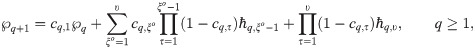 Figure 5
 Figure 6
 Figure 7
 Figure 8
 Figure 9
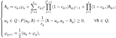 Figure 10
 Figure 11
 Figure 12
 Figure 13
 Figure 14
 Figure 15
 Figure 16
 Figure 17
 Figure 18
 Figure 19
 Figure 20
 Figure 21
 Figure 22
 Figure 23
 Figure 24
 Figure 25
 Figure 26
 Figure 27
 Figure 28
 Figure 29
 Figure 30
 Figure 31
 Figure 32
 Figure 33
 Figure 34
 Figure 35
 Figure 36
 Figure 37
 Figure 38
 Figure 39
 Figure 40
 Figure 41
 Figure 42
 Figure 43
 Figure 44
 Figure 45
 Figure 46
 Figure 47
 Figure 48
 Figure 49
 Figure 50
Peer Reviews
No public reviews on file for this paper yet. If you reviewed it on a platform where reviews are public (OpenReview, ICLR, NeurIPS, ICML), you can paste yours below so the community can read it here.
Videos
No videos yet. Explain this paper in a talk, walkthrough, or lecture? Add one.
Taxonomy
TopicsOptimization and Variational Analysis · Fixed Point Theorems Analysis · Advanced Optimization Algorithms Research
1 Introduction
In a fast developing area of nonlinear theory of differential equation, control theory, image recovery, game theory, etc,. many indispensable results have been established by the use of nonlinear functional analysis based on fixed point theory. In the recent past, fixed point theory has grown into a full fledged research area. Several notions associated with fixed point theory, which can be used to generate a particular elegant approach for the solution of nonlinear problems arising in mathematics, statistics, engineering, economics, approximation theory, theory of differential equations, theory of integral equations, etc., has been established in the contemporary literature (see, for example, [1] and the references therein).
After the initial impetus provided by Nadler [2] in 1969, unwavering attention has been given to the study of fixed point theorems for multivalued mappings. This stem from the significance of fixed point theory for this class of nonlinear mappings in different fields. Other interesting results that followed the remarkable conclusion obtained in [2] with respect to multivalued contraction mappings include, but not limited to the following: Markin [3] initiated the concept of employing Hausdorff metric to examine the fixed points of certain multivalued contraction and nonexpansive mappings, Hu et al [4] proved theorems concerning common fixed points of two multivalued nonexpansive mappings satisfying appropriate contractive inequalities, Bunyawat and Suntain [5] originated a method of establishing common element of solution for a countable family of multivalued quasi-nonexpansive mappings in a uniformly convex Banach space, Isogugu [6] initiated the concept of type-one ϑ-SPM which assures strong convergence without imposing any condition on the fixed point set, Agwu and Igbokwe [7] introduced a technique for obtaining common element of solution for minimization problems with fixed point constraint, etc.
However, we were being captivated by the following techniques studied in [9]: Let H be a real Hilbert space and ∅ ≠ Q ⊂ H be convex and closed. Given the point ℘0 ∈ Q and for each , let ( is a countable family of type-one -SPM (defined below). The Mann-type technique developed by {℘q} is
where for each ξ^o^. If is a bifunction fulfilling (B1) − (B4) and be as described above for each , then the modified lshikawa technique developed from {℘q} is given by
where for some a > 0, {rq} ⊂ [a, ∞).
Our captivation is basically because of the introduction of the new schemes ((1) and (2)) that address the setbacks (sum conditions) which restricted the application of many results published in this direction.
Subsequently, an unwavering attention has be drawn to methods incorporating several auxiliary maps (see, for example, [8] for details) which is known to be more robust against certain numerical errors as compared to those that involve only one auxiliary mapping. In view of this, the following question becomes necessary:
Question 1.1 Can we obtain a method involving several auxiliary mapping which guarantees strong convergence for certain class of multivalued mappings?
Moltivated and inspired by several works studied, and in particular the remarkable conclusions in [9], our focus in this paper are the following:
(a) To intiate the notion of ϑ-SAPM in a real Hilbert space domain;(b) To address the request of Question 1.1 above.(c) To establish strong convergence theorem involving equilibrium problems and mixed-type fixed point problems.
2 Relevant preliminaries
In what follows, the following concepts and known results will be required in order to prove our main results: Let H be a real Hilbert space H with the inner product 〈, ., 〉 and the norm ‖.‖ and ∅ ≠ Q ⊂ H be a convex and closed. Throughout the remaining sections in this paper, the following symbols shall be used: will represent the set of natural numbers, will represent the set of real numbers and ⇀ and → will represent weak and strong convergence of any sequence in H, respectively.
Let ℑ, ð: Q → Q be two nonlinear mappings. We shall use F(ℑ), F(ð) and to denote the set of fixed points of ℑ and ð and the set common fixed point of ℑ and ð, respectively.
Definition 2.1 Recall that
(a) ℑ is known as an asymptotically strict pseudocontraction (ASPM, for short) if and a ϑ ∈ [0, 1) that guarantees
The class of mappings represented by (3) is a superclass of the class of asymptotically nonexpansive mappings (ANM, for short) (where ℑ is known as ANM if for all ℘, ℏ ∈ Q, which assures the inequality ‖ℑ^q^℘ − ℑ^q^ℏ‖ ≤ νq‖℘ − ℏ‖, ∀q ≥ 1) studied in [10].Remark 2.1 It is worthy to mention that if F(ℑ) ≠ ∅, then (3) becomes an asymptotically demicontractive mapping (ADM, for short).(b) ℑ is known as k-strictly pseudocontractive if there exists a constant ϑ ∈ [0, 1) such that for all ℘, ℏ ∈ Q, we have
This class of k-strictly pseudocontractive has been extensively studied by several authors (see, for example, [7, 8, 11, 12] and the reference therein). It is shown in [13] that a strictly pseudocontractive map is L Lipschitzian (i.e., ‖ℑ℘ − ℑℏ‖ ≤ L‖℘ − ℏ‖ for all ℘, ℏ ∈ D(ℑ)) in [14] that the class of k-strictly asymptotically pseudocontractive maps and the class of strictly pseudocontractive maps are independent.(c) ℑ is called uniformly L-Lipschitzian if there exists a constant L > 0 such that
and is said to be demiclosed at a point ν if whenever is a sequence in D(ℑ) such that converges weakly to ℘^⋆^ ∈ D(ℑ) and converges strongly to ν, then ℑ℘^⋆^ = ν.
Let be a bifunction. An EP for ℧ is to search for an ω ∈ Q that assures the inequality
A point z ∈ Q is referred to as an equilibrium point if it solves problem (5).
We shall use EP(℧) to indicate the solution set of problem (5); that is,
Considering the invaluable position of equilibrium problems in real life applications, several methods have been deployed to approximate the solution of problem (5); see [15] for more detail. In recent past, different authors have investigated joint problems involving equilibrium and fixed point problem of one mapping in the Hilbert space domain; see, for instance, [5, 9, 15–19] and the references contained in them.
Let B denote a strong positive bounded linear operator on a real Hilbert space domain H; that is, it is possible to get a constant which assures that inequality
The problem here is to minimize a quadratic function over the set of fixed points of a nonexpansive mapping τ in a real Hilbert space domain:
given that b ∈ H.
In view of the above, and motivated the results in [20], Marino and Xu [21] initiated the following method for approximating the fixed point of nonexpansive mapping via viscosity technique initiated by Moudafi [22]:
where ℑ and f represent nonexpansive and contraction mappings, respectively. Using (7), they obtained a strong convergence to the unique solution of the variational inequality problem
which represents the optimality condition for the minimization problem
with denoting the potential function of γf (i.e., .
Generally, approximating fixed points of single-valued mappings is simpler compared to its multivalued counterpart. However, several researchers have continued to investigate different methods of obtaining invariant point of multivalued mappings, reasons basically contained in their involvement in several real world applications including optimisation and variational inequalities problems (see [2, 3, 23–28]).
A subset Q of a normed space Δ is considered as being proximinal if it is possible to find a point ϕ ∈ Q which assures
for each ℘ ∈ Δ. It has been established that a subset of a real uniformly convex Banach space admitting closedness and convexity properties and a subset of a real Banach space guaranteeing convexity and weakly compactness properties are both proximinal.
In what follows, CB(Δ), C(Q) and shall represent the family of nonempty bounded closed subsets of Δ, the family of nonempty compact subsets of Q and the family of nonempty bounded proximinal subsets of Q, respectively. The Hausdorff metric induced by the metric ρ of Δ for all A, B ∈ CB(Δ) is given as
where ρ(℘, B) = inf{‖℘ − ℏ‖ : ℏ ∈ B} denotes the distance from the point ℘ to the subset B. A point ℘^⋆^ ∈ Q is said to be a fixed point of the multivalued mapping ℑ if ℘^⋆^ ∈ ℑ℘^⋆^. T Denote by F(ℑ) = {℘ ∈ Q : ℘ ∈ ℑ℘} the set of fixed points of ℑ
Definition 2.2 The ℑ : D(ℑ) ⊆ Δ → 2^Δ^ is known as:
uniformly L-Lipschitzian it it is possible to get an L ≥ 0 which assures
If L = νq in (11), where , then ℑ becomes ANM.type-one [6] if ∀℘, ℏ ∈ D(ℑ), we get
where .ϑ-strictly asymptotically pseudocontraction (ϑ-SAPM) if it is possible to find a sequence and a k ∈ [0, 1) in which, for any pair ℘, ℏ ∈ D(ℑ) and an a ∈ ℑ^q^℘, ∃b ∈ ℑ^q^ℏ assuring ‖a − b‖ ≤ Θ(ℑ^n^℘, ℑ^q^ℏ) and
If ϑ = 1 in (13) then ℑ becomes asymptotically pseudocontractive; whereas ℑ reduces to ANM if ϑ = 0 in (13).
Very recently, Isogugu [29] introduced the following nonlinear map in the Hilbert space domain:
Definition 2.3 Let X be a normed space and ℑ : D(ℑ) ⊆ X → 2^X^ be a given map. Then ℑ is known as ϑ-strictly pseudocontractive-type in the sense of Browder and Petryshyn [30] if there exists ϑ ∈ [0, 1) such that given any ℘, ℏ ∈ D(ℑ), and a ∈ ℑ℘, we can find b ∈ ℑℏ satisfying ‖a − b‖ ≤ Θ(ℑ℘, ℑℏ) and
Note that ℑ in (14) becomes pseudocontractive-type if ϑ = 1 and nonexpansive-type if ϑ = 0. It is not hard to see from (14) that every nonexpansive-type multivalued mapping is ϑ-strictly pseudocontractive-type and every ϑ-strictly pseudocontractive type multivalued mapping is pseudocontractive-type. It is shown in [29] that the class of nonexpansive-type and ϑ-strictly pseudocontractive-type multivalued mappings are properly contained in the class of ϑ-strictly pseudocontractive-type and pseudocontractive-type multivalued mappings, respectively.
Definition 2.4 [6] Let E be a Banach space and ℑ : D(ℑ) ⊆ E → 2^E^ be a multivalued mapping. I − ℑ is said to be weakly demiclosed at zero if for any sequence such that {℘n} converges weakly to ν and a sequence with ℏ_n_ ∈ ℑ℘n for all such that {℘n − ℏ_n_} strongly converges to zero. Then, ν ∈ ℑν(i.e., 0 ∈ (I − ℑ)ν).
Lemma 2.1 1001 [21] Consider a bounded linear mapping A on H which assures strongly positive self adjoint (with the coefficient ϰ > 0 and 0 < ϱ ≤ ‖A‖^−1^), then ‖1 − ϱA‖ ≤ 1 − ϱϰ.
Lemma 2.2 1001 [12] Let H be as described above. Then
Lemma 2.3 (see 1001 [20]) Let {φn} ⊂ [0, ∞) with φn+1 = (1 − αn)φn + σn, n ≥ 0, where {αn} ⊂ (0, 1) and {σn} is a sequence in R such that and . Then, lim_n→∞_ φn = 0.
Lemma 2.4 1001 [31] For each ℘1, ℘2, ⋯, ℘m and α1, α2, ⋯, αm ∈ [0, 1] with , we have
Lemma 2.5 1001 [32] Let {ℏ_r}r≥1_ be a sequence of real numbers that does not decrease at infinity. In addition, consider the sequence of integers defined by
Then, is a nondecreasing sequence verifying and for all r ≥ r0, the following two inequalities hold:
For solving the equilibrium problem, we take the following assumptions into consideration: the function ℧ : Q × Q → R satisfies the following conditions:
(M1) (M2) ℧ is monotone, i.e, (M3) ℧ is upper hemicontinuous, i.e., for each ℘, ℏ, z ∈ Q,
(B4) is convex and lower semicontinuous for each ℘ ∈ Q.
Lemma 2.6 1001 [33] Let H be a real Hilbert space H, ∅ ≠ Q ⊂ H be closed and convex and let ℧ be a bifunction of Q × Q assuring (M1) − (M4). For r > 0, and given , we can find that guarantees the inequality
Lemma 2.7 1001 [15] Assume that assures (B1) − (B4). Define an a operator ℑ_r_ : H → Q as
where r > 0. Subsequently,
(i) ℑ_r_ is single-valued;(ii) for any ℘, ℏ ∈ H,
(iii)
Proposition 2.1 1001 [9] Let be a countable subset of , where s is a fixed nonnegative integer and υ is any integer with s + 1 ≤ υ. Then, the following identity holds:
Proposition 2.2 1001 [9] Let t, u, v ∈ H be arbitrary. Let s be any fixed nonnegetive integer and be such that s + 1 ≤ υ. Let and . Define
Then,
where and wq = (1 − cq)v.
Recently, Rizwan et al. [34–38] worked on several types of fixed point algorithms, HR-Ciric-Reich-Rus contractions, generalized enriched contractions, and MR-Kannan-type interpolative contractions. They provide very important applications of fixed point theory including activation functions through fixed-circle problems.
3 Main results
Definition 3.1 Let X be a normed space and ℑ : D(ℑ) ⊆ X → 2^X^ be a given map. Then, ℑ is k-ASPM in the thought of Isogugu et al. [9] if there exists μ ∈ [0, 1) such that given any ℘, ℏ ∈ D(ℑ) and uq ∈ ℑ^q^℘, we can find with and vq ∈ ℑ^q^ℏ satisfying for which
Remark 3.1 From Definition 3.1, it is not difficult to see that every multivalued nonexpansive-type mapping is strictly asymptotically pseudocontrctive-type mapping. The examples below show that the class multivalued nonexpansive-type mapping is properly included into the class of multivalued strictly asymptotically pseudocontrctive-type mapping and the class of multivalued strictly asymptotically pseudocontractive-type mapping is properly included into the class of asymptotically pseudocontrctive-type mapping.
Example 3.1 (see [39]) Give the usual metric and let the map be given as
Then, for n odd (q ≥ 2), we obtain
Now,
Also, for each . Choose vq = −δ^q^ℏ. Then
and
From (19) and (20), we obtain
The following example shows that the class of θ-strictly asymptotically pseudocontractivetype multivalued mapping is more general than the class of asymptotically nonexpansive-type mappings.
Example 3.2 Let be endowed with the usual metric and define the mapping by
Then, for n odd q ≥ 2, we get
Then, for all ℘ ∈ [−1.5, 1] and hence it is not ANM. Indeed,
Observe that for each . Choose vq = −δ^q^ℏ so that
and
Now,
Therefore, ℑ is k-SAPM with kn = 1 and . Note that ℑ, not being ANM, demonstrates the conclusion that the class of ANM mappings is properly included into the class of k-SAPM.
Now, we show with the following examples that the class of multivalued asymptotically strictly pseudocontractive-type mappings and the class of multivalued strictly pseudocontractive-type mappings are independent.
Example 3.3 Let be endowed with the usual metric and define by
It is shown in [29] that ℑ is a strictly pseudocontractive-type mapping.
For q even (q > 1), we have
Observe that for each . Choose vq = δ^q^ℏ so that
and
Now,
where k = 0 and νq = 1. Hence, ℑ is not asymptotically k-strictly pseudocontractive-type.mapping.
Example 3.4 Let and let . Define by
where is a real sequence satisfying a2, a3 > 0, 0 < at < 1, t ≠ 2, 3 and . Then,
for all k ∈ (0, 1), n ≥ 1 and , where . Since , it follows that ℑ is asymptotically pseudocontractive-type.
Now, choose and a3 = 4, then we get
where and . Hence, ℑ is not strictly pseudocontractive-type.
Now, we shall prove the strong convergence of the new method to the solution set of an equilibrium problem (EP) and the set of common fixed points of two finite families of type-one (θ-SAPM) and θ-strictly pseudocontractive-type multivalued mapping (θSPM).
Theorem 3.1 Let H, Q and ℧ be as described above. Suppose and , υ ≥ 2 are finite families of type-one and -uniformly Lipschitizian strictly asymptotically pseudocontractive-type and type-one strictly pseudocontractive-type multivalued mappings, respectively, with contractive coeficient for each ξ^o^. Suppose and for each ς, and are weakly demiclosed at zero. let be a ρ-contraction self map of Q with ρ ∈ (0, 1) and A be a strong positive self adjoint bounded linear operator on H with coeficient such that . Let be a sequence developed from an arbitrary ℘0 ∈ Q by
where and for each ξ^o^, {αq}, {δq} ∈ [0, 1], . Suppose the requirements below are fulfilled:
(i) for each i;(ii) and (iii) and (iv) and (v) {rq} ⊂ [a, ∞) for some a > 0.
Then, the sequence given by (23) admits strong convergence to , which provides a solution to .
To start with, we establish the fact that the operator is a self contraction map of Q. Given and for all ℘, ℏ ∈ H, it follows from Lemma 2.5 with and that
Therefore, we can find a unique point ℘^⋆^ ∈ Q for which which we can write as
Since αq → 0 as q → ∞, we can take ∀q ≥ 0. Using condition (iv), it is possible to get a constant ϵ with 0 < ϵ < 1 − δ and for each ς. Also, by Lemma 2.1, we get .
Let and . Since and we obtain (using Lemma 2.7) that
Further, we prove that is bounded. Since is k-SAPM and k-SPM, F(ℑ) ≠ ∅ and . Consequently, we can find a sequence and real positive constants such that for any we obtain
and
By (23) and Proposition 2.1 with sq = η, ωq = t, ℘^⋆^ = u, s = 1 and we have
Since is type-one k-SAPM, we have, using (30), that
From Proposition 2.2, it follows, for s = 1, that
Also, from (23) and Proposition 2.2 with ωq = η, uq = t, ℘^⋆^ = u, s = 1 and , it is not difficult to see (employing the same approach as in above) that
From (31) and (32), we obtain
Also, using (23), we obtain the following estimates:
By applying conditions [(i) and (iv)] in (33), we get
From (35) and (36), we obtain
Employing mathematical inductional argument, we have
The last inequality implies that the sequence is bounded; and as a consequence, the boundedness of the following sequences: and are assured.
Next, for each i, we prove the following conclusion: ‖ωn − πn,i‖ → 0 and as q → ∞. Using Lemma 2.1, (34) and (36), we get the following estimates:
By setting
The inequality above becomes
To established that ℘q → ℘^⋆^ as q → ∞, consider the two Cases below:
Case A: Let be monotonically decreasing. Then, is convergent. Therefore,
Hence, (40) and (41) in company with (i), (ii), (iv) and the characteristic property of {νq} give
Since it follows from (42) that
Applying the same line of thought as in above (taking into account (40) and (41), (i), (iii), (iv) and the characteristic property of {νq}), it will not be difficult to see that
Since employing (44) we have
Next, we prove that . For any we get
so that
From (31), (32) and (36), we have
which by (46) gives
where , and .
Using (41), condition (iv) and the characterization of {νq}, we get from the last inequality that
Furthermore, the following estimates are due to the application of (23) and Proposition 2.2:
and by using (23), Proposition 2.2 and (42), we have
Now, observe that
which by (48), (49), (50) and (51) yields
Also, observe that
which, from (45), (48), (49), (50) and (51), we obtain
Next, we prove that
where represents a unique solution of the variational inequality (8). To start with, select a subsequence of such that
Now, consequent upon the bounded of the sequence (as shown above), we can find a subsequence of such that as k → ∞. Since ‖uq − ℘q‖ → 0 as q → ∞, it follows that . We prove that .
To start with, we prove that ξ^o⋆^ ∈ EP(Ψ). By uq = Trq℘n, we get
Using (B2), we also obtain
which consequently becomes,
Since and , from (B4), we obtain
Let ℏ_t_ = tℏ + (1 − t)ξ^o⋆^, where ℏ ∈ Q and t ∈ (0, 1]. Since ℏ, ξ^o⋆^ ∈ Q and Q is convex, we get ℏ_t_ ∈ Q and ℧(yt, ξ^o⋆^) ≤ 0. Therefore, from (B1)and (B4), we get
which yields ℧(ℏ_t_, ℏ) ≥ 0. Using (B3), we get ℧(ξ^o⋆^, ℏ) ≥ 0, ∀ℏ ∈ Q. Thus, ξ^o⋆^ ∈ EP(℧).
Now, from , and the demiclosedness property of for each ς, and by applying standard argument, we have that . In addition, since and lim_q→∞_ ‖uq − sq‖ = 0, we immediately obtained from the demiclosedness property that . Hence, . Since and , we get from (55) that
as required.
Since from (23) and Lemma 2.2
it follows from (25), (31) and (32) that
where ϖ, ϖ^⋆^ and ϖ^⋆⋆^ are still as described above.
From the last inequality, we obtain that
Set
and
Then, from (59), we have that
where bq = ‖℘q − ℘^⋆^‖^2^. It is not difficult to see, from (iv) and the fact that , that
Thus, from Lemma 2.3 and (60), .
Case B: Suppose {‖℘q − q‖} is monotonically increasing. Then, the integer sequence (for some q0 large enough) can be written as
It is easily seen that {τq} is nondecreaing sequence and for all q ≥ q0, we have
From (40), (43), (48) and (43) with (q replaced by τ(q)), we obtain
and
By using similar argument as in Case A, we have
κτ(q) → 0 as and . Therefore, from Lemma 2.3, we obtain lim_n→∞‖℘τ(q)_ − ℘^⋆^‖ = 0 and .
Hence, by Lemma 2.5, we get
Hence, converges to and the proof is completed.
Next, using our main result (Theorem 2.1), we prove strong convergence theorem for finding a solution of the variational inequality problems in the setup of real Hilbert spaces.
Theorem 3.2 Let and fς be as given in Theorem 3.1. Let be a sequence developed from an arbitrary ℘0 ∈ Q by
where and for each ξ^o^, {αq}, {δq} ∈ [0, 1] and . Suppose the requirements below are fulfilled:
(i) for each ξ^o^;(ii) and (iii) and (iv) and .
Then, as q → ∞, which provides a solution to the variational inequality .
If ℧(℘, ℏ) = 0 ∀℘, ℏ∈Q, r = 1 ∀q ≥ 0, then uq = ℘q. Therefore, with f(℘) = v and A = I, the conclusion is a consequence of Theorem 3.1.
4 Numerical example
Now, we present a numerical example to support to demonstrate the efficiency of our suggested method.
Example 4.1 Let Q = [−3, 3] and . For each ξ^o^ = 1, 2, 3, let and , be given as
and
It is shown in [11] that ℑ is a k-SPM. Also, it is easy to see from Example 3.1 above that ð is k-SAPM. In addition, for n odd (q ≥ 2), we obtain
On the other hand, let the bifunction ℧ be given as
It is easy to see that ℧ fulfills conditions (B1) − (B4). Set rq = q + 1, then , where q ≥ 1 (see [40] for more information). For N = 3, (23) becomes
Put and . Then, for arbitrary ℘0 ∈ Q, the above iteration scheme yields:
where for ℘q ∈ (−3, 0] whereas if ℘q ∈ (−3, 0].
Observe that the sequence ℘q → 0 as q → ∞. To be precise, .
5 Conclusion
In this manuscript, we introduce a new class of mappings (θ-SAPM) and propose a novel method for solving equilibrium problem with mixed fixed point constraints. We establish strong convergence result of the proposed technique without any imposition of sum conditions on the iteration parameters (hence less computational cost). In addition, we showed that the class of θ-SPM and the class of θ-SAPM are independent. Also, we illustrated the convergence of our method through numerical experiment. Our future project will consider some comparison test of our technique with some existing techniques that probably imposes sum conditions on the iteration parameters.
The reference list from the paper itself. Each links out to its DOI / PubMed record.
- 1Bharucha-Reid A. T., Random integral equations, Academic Press, New York, 1972.
- 2Nadler S.B., Multivalued mappings, Pac. J. Math., 30 (1969), pp.475–488. doi: 10.2140/pjm.1969.30.475 · doi ↗
- 3Markin J.T., Continuous dependence of fixed point sets, Proc. Amer. Math. Soc., 38 (1973), pp.547–547. doi: 10.1090/S 0002-9939-1973-0313897-4 · doi ↗
- 4Hu T., Huang J. and Rhoades E., A general principle for lshikawa iteration for for multivalued mappings, Indian J. Pure Appl. Math., 28 (1997), pp.1691–1098.
- 5Abkar A. and Tavakkoli M., Anew algorithm for two finite families of demicontractive mappings and equilibrium problems, Appl. Math. Comput., 266 (2015), pp.491–500.
- 6Isiogugu F.O., On the approximation of fixed points for multivalued pseudocontractive mappings in Hilbert spaces, Fixed Point Theory Appl., 2016 (2016), 59 pages. doi: 10.1186/s 13663-016-0548-x · doi ↗
- 7Agwu I.K. and Igbokwe D.I., A Modified proximal point algorithm for finite families of minimization problems and fixed point problems of asymptotically quasi-nonexpansive multivalued mappings Punjab University Journal of Mathematics, 54(8) (2022), pp.495–522. doi: 10.52280/pujm.2022.540801 · doi ↗
- 8De la sen M., On some convergence properties of the modified lshikawa scheme for asymptotically demicontractive mappings with metricial parameterizing sequences, Hindawi J. Math., 2018 (2018), 13 pages.