Golden eagle optimized fractional-order PI controller design for a PFC SEPIC converter in EV charging
S. Vijayakumar, N. Sudhakar

TL;DR
This paper introduces a new method using Golden Eagle optimization to design a better controller for electric vehicle chargers, improving performance and stability.
Contribution
The novelty lies in applying Golden Eagle optimization to tune a fractional-order PI controller for a SEPIC converter in EV charging.
Findings
The optimized FOPI controller reduces settling time and inrush current in the converter.
The system shows faster dynamic response and lower harmonic distortion compared to conventional methods.
Simulation results confirm improved stability and performance using the proposed optimization technique.
Abstract
The power factor correction converter is the function of the front-end converter, followed by the DC–DC converter of the electric vehicle charger. It improves the power factor and regulates the output voltage and current. This research article proposes the Golden Eagle optimization for fractional order PI (FOPI) controller for Single Ended Primary Inductor Converter (SEPIC) power factor correction. The Golden eagle optimization is based on its knowledge of hunting tactics at various degrees of spiral trajectories to catch the prey. The FOPI controller has a broad range of controller parameters that provide better control and performance of the converter. The tuning of the parameters of the FOPI controller is optimized in Golden Eagle Optimization, and the Integral Absolute error with Integral Square error is used for the objective function. The optimized parameters of FOPI compare with…
Genes, proteins, chemicals, diseases, species, mutations and cell lines named across the full text — each resolved to its canonical identifier and authoritative record.
Click any figure to enlarge with its caption.
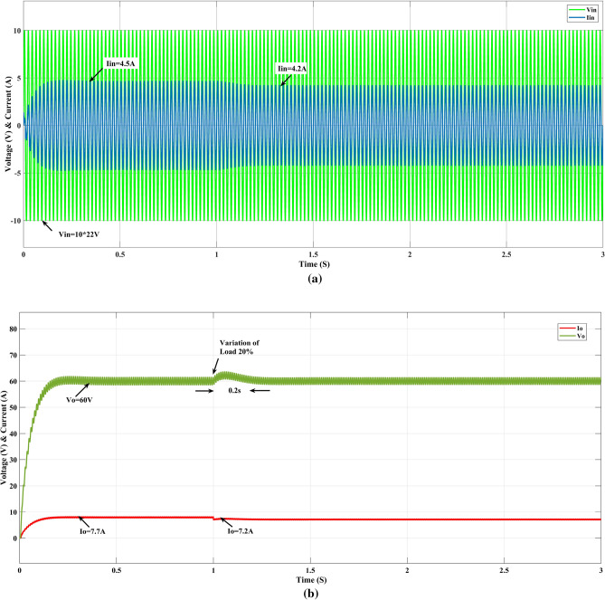 Figure 10
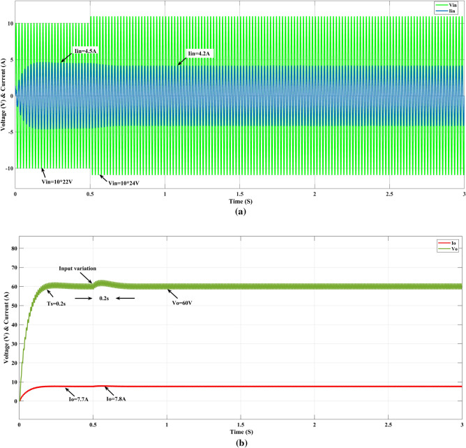 Figure 11
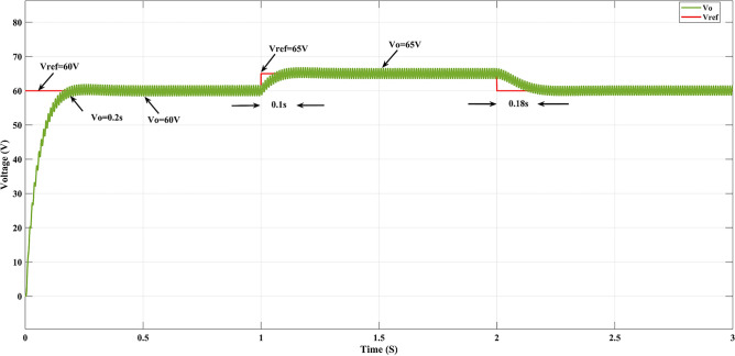 Figure 12
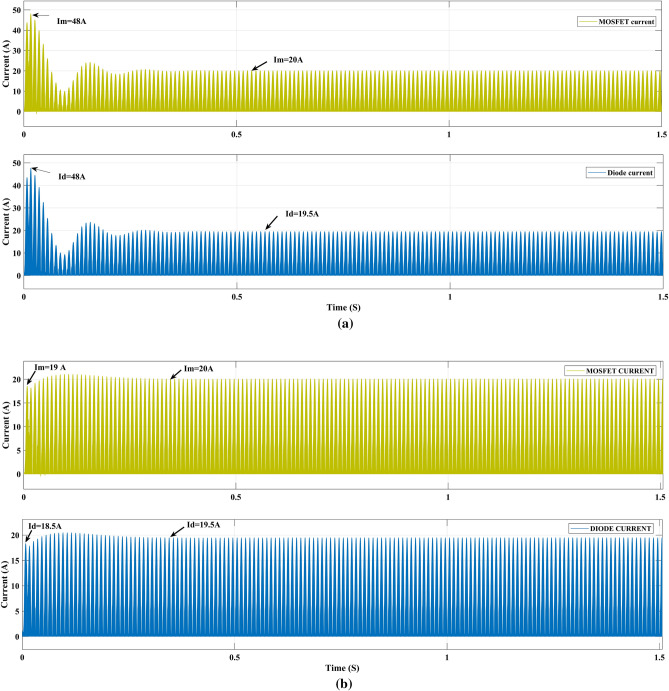 Figure 13
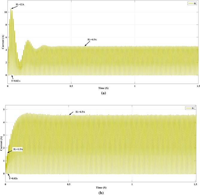 Figure 14
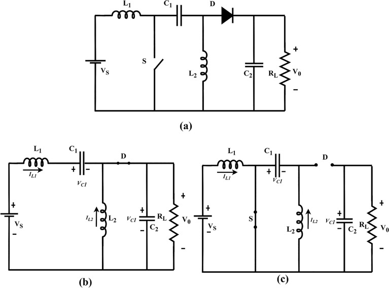 Figure 1
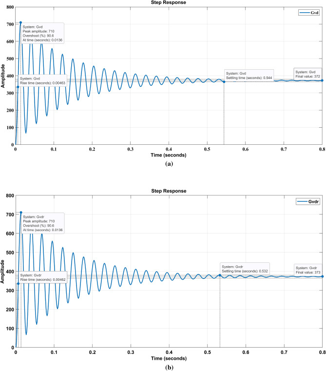 Figure 2
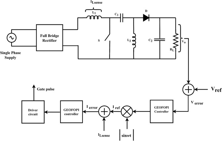 Figure 3
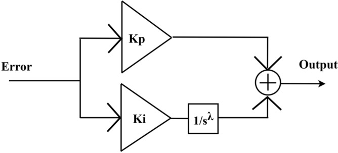 Figure 4
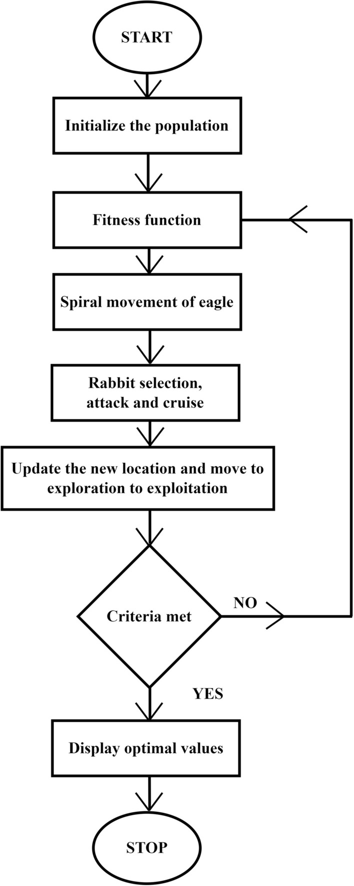 Figure 5
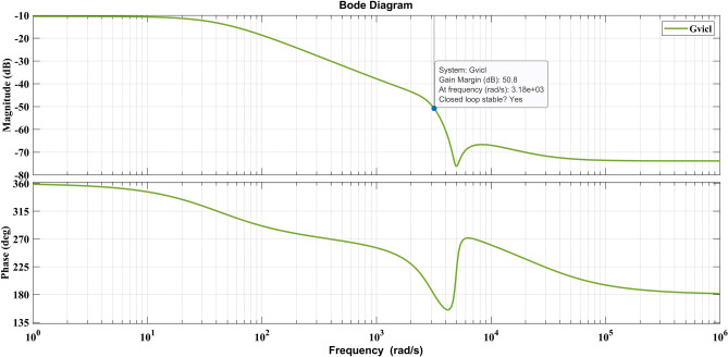 Figure 6
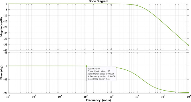 Figure 7
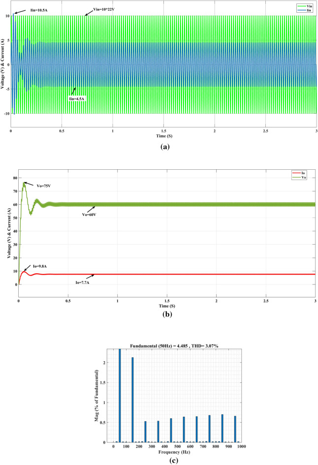 Figure 8
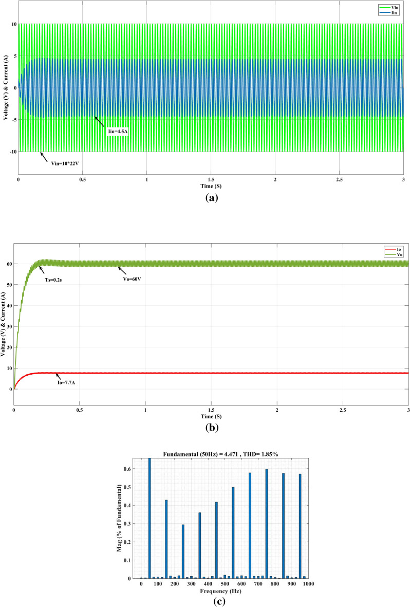 Figure 9
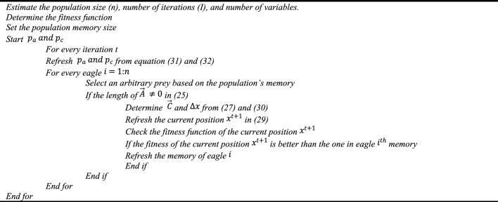 Figure 15
- —Vellore Institute of Technology, Vellore
Peer Reviews
No public reviews on file for this paper yet. If you reviewed it on a platform where reviews are public (OpenReview, ICLR, NeurIPS, ICML), you can paste yours below so the community can read it here.
Videos
No videos yet. Explain this paper in a talk, walkthrough, or lecture? Add one.
Taxonomy
TopicsReligious and Theological Studies · Educational theories and practices · Spanish Philosophy and Literature
Introduction
The Fuel demand, fossil fuel reserves, and the subsequent increase in fuel prices and emissions of greenhouse gases have put the transportation industry at the epicentre of the climate disaster^1^. Hybrids, electric automobiles, fuel cell vehicles, and solar-powered vehicles contribute to a cleaner environment and less greenhouse gas emissions^2^. Battery chargers are classified as On-board and OFF-board chargers. Off-board charges can only be found at certain places, like fuel stations, and it is possible to charge rapidly with these chargers, but it renders the battery overheated^3^, and the life span is minimal. Concerns about the electric vehicle range and the battery performance are two main obstacles to its broad use. The lack of charging stations and infrastructure also demands On-board chargers (OBC). The PFC converter is an integral part of the OBC charger that transforms the grid supply alternating current into direct current for vehicle battery charging. The boost converter has attracted widespread attention, and the issues with bulky components require a filter at the output and high voltage stress^4^. The Buck converters are less expensive and more efficient, but dead angle issues mainly influence them in supply voltage and need an input filter^5,6^. DC–DC Cuk converters are good at isolation, current limiting, and short-circuit protection. Moreover, two major drawbacks are the severe current stress felt across the switch and the reversed polarity when loaded^7^. An isolated converter, such as flyback, push–pull, and forward converter, is in AC–DC conversion and has problems with size, transformer core saturation, non-minimum phase and current harmonics drawbacks^8^. Non-isolated converter topologies are often selected because of the absence of transformers, and their benefits include low cost, compactness, lightweight, good efficiency, and minimum losses. The SEPIC converter may alleviate the shortcomings of the Cuk converter, Buck converter, and Boost converter, and it has a faster transient response than other converters. These critical points of the SEPIC converter are more appropriate for power factor correction applications when charging a battery.
The behaviour of DC–DC converters is not linear, and this behaviour changes when the parameters are changed^9^. The small-signal model-based controllers for DC–DC converters are inadequate in meeting the stability requirements, needed regulation, and transient responsiveness for significant load variations. To regulate the output voltage, the cascade control technique for single-stage active power factor correction (PFC) utilizes the use of an outer voltage controller. An inner current controller is also used to shape the input current, and the PI controller is employed for this purpose. Many fine-tuning methods have been proposed to improve the feedback system and be more reliable. The PI and PID controls are well-known and used in many fields. They are easy to set up and work on average^10^. PID controllers are mostly insignificant owing to parametric unpredictability and various disturbances^11^. The fractional order controller is sensitive to both dynamic load and requirements, and it has two extra factors on top of the current PID that make it more flexible while still sturdy. It ensures the optimal result for higher-order non-linear systems without a minimum phase. The capacity of fractional order (FO) controllers to endure unpredictability and load disturbance is an essential feature^12^. Because of their increased adaptability, these controllers can better satisfy design criteria such as phase margin and gain, resistance to parameter variations, and more. Because of these characteristics, fractional order controllers can successfully regulate power converters and other non-linear facilities^13^. In the boost converter^14^, Compared to the integer-order controller, the fractional-order controller performs better in overshoot and recovery time in both simulations and experiments. FOPID controller is implemented to minimize vibration, noise, and harmonic current of three-phase induction motors^15^ and controller parameter design with motor specifications. The fractional order PID (FOPID) control scheme needs more accurate and effective tuning than general tuning methods, and this technique improves settling time, lowers overshooting, and lowers the steady-state error of the system. Many research studies are actively using optimization-based metaheuristic algorithms for power electronic applications.
From the literature survey, the converging time of genetic algorithms (GAs) is higher than average because of the randomness of the cross-over and mutation processes^16^. Particle Swarm Optimization (PSO) is used in PI tuning, but it has a significantly low convergence rate and settling times for the converter^17^. Grey wolf optimization has many constraints over convergence and poor searching performance^9^. The Firefly and bacterial foraging optimization are used for PID controller for the converter side, but it has the drawback of being stuck in several local optima solutions^18^. The Golden Eagle Optimisation Algorithm (GEOA) has benefits over other methods^19^ and is a powerful and bio-inspired optimization technique that can find the best global parameters for the outer and inner controllers of the PFC SEPIC converter. The controllers regulate the output voltage quickly and effectively, and the input current is shaped to improve the power factor at the supply side. Hence, the system performance is enhanced, such as virtually UPF, low percentage of THD, and shorter settling time for line, load, and setpoint variations. The GEO tunned FOPI is used in the closed loop cascade control strategy. The THD level is significantly low value, the power factor reaches near unity, and the initial inrush current at switches and the input side is minimal.
The significant contributions of this work are as follows
- Fast dynamic response on variation in input and load
- Reduction of initial inrush current in switching devices and inductor
- Achieve the high-power factor and lower THD
The GEO fractional-order PI controller design for a PFC SEPIC converter in EV charging introduces a pioneering approach to power electronics and EV charging systems. By integrating the GEO technique with FOPI control, the proposed method enhances the performance and efficiency of power factor correction (PFC) SEPIC converters utilized in EV charging infrastructure. This innovation offers superior adaptability to varying load conditions, increased stability, and optimized energy conversion, thereby advancing the efficacy and sustainability of EV charging technologies. This paper is organized into five parts as follows, “Mathematical modelling and design” discusses converter mathematical modelling and design, "Closed loop operation of PFC converter" discusses the closed loop operation of PFC converter, "Simulation results and discussion" is the simulations results and discussion, and finally, the conclusion about the research studies of this paper in the "Conclusion".
Mathematical modelling and design
Modelling of SEPIC converter
The circuit of the SEPIC converter shown in Fig. 1 consists of a MOSFET switch S, diode D, an input and output inductor L_1_ & L_2_, an energy transfer capacitor C_1_, an output filter capacitor C_2_, D is the freewheeling diode and a load resistor (R_L_). When the switch S closes, i_L1_ flows through the inductor L_1_ and charges. Equations (1), (2), and (3) represent the steady state and transient currents and voltages. The state model of the SEPIC converter is derived to obtain the mathematical model of the converter by considering that the switch is ‘ON’, (i.e.) S = 1 during the MOSFET switch conduction subinterval and switch is ‘OFF’ (i.e.) S = 0 during the diode conduction subinterval. State-space averaging is used to depict the dynamics of the converter, and the state equations at switch S = 1 and S = 0 are combined using as follows:Figure 1**(a)** SEPIC converter**, (b)** OFF-state**, (c)** ON-state.
\documentclass[12pt]{minimal} \usepackage{amsmath} \usepackage{wasysym} \usepackage{amsfonts} \usepackage{amssymb} \usepackage{amsbsy} \usepackage{mathrsfs} \usepackage{upgreek} \setlength{\oddsidemargin}{-69pt} \begin{document}$$\left[\begin{array}{c}\frac{d{I}_{L1}}{dt}\\ \frac{d{I}_{L2}}{dt}\\ \frac{d{V}_{C1}}{dt}\\ \frac{d{V}_{C2}}{dt}\end{array}\right]=\left[\begin{array}{cccc}0& 0& 0& 0\\ 0& 0& \frac{1}{{L}_{2}}& 0\\ 0& \frac{-1}{{C}_{1}}& 0& 0\\ 0& 0& 0& \frac{-1}{{R}_{L}{C}_{2}}\end{array}\right]\left[\begin{array}{c}{I}_{L1}\\ {I}_{L2}\\ {V}_{C1}\\ {V}_{C2}\end{array}\right]+\left[\begin{array}{c}\frac{1}{{L}_{1}}\\ 0\\ 0\\ 0\end{array}\right]\left[{V}_{in}\right]$$\end{document} \documentclass[12pt]{minimal} \usepackage{amsmath} \usepackage{wasysym} \usepackage{amsfonts} \usepackage{amssymb} \usepackage{amsbsy} \usepackage{mathrsfs} \usepackage{upgreek} \setlength{\oddsidemargin}{-69pt} \begin{document}$$\left[\begin{array}{c}\frac{d{I}_{L1}}{dt}\\ \frac{d{I}_{L2}}{dt}\\ \frac{d{V}_{C1}}{dt}\\ \frac{d{V}_{C2}}{dt}\end{array}\right]=\left[\begin{array}{cccc}0& 0& \frac{-1}{{L}_{1}}& \frac{-1}{{L}_{1}}\\ 0& 0& 0& \frac{-1}{{L}_{2}}\\ \frac{1}{{C}_{1}}& 0& 0& 0\\ \frac{1}{{C}_{2}}& \frac{1}{{C}_{2}}& 0& \frac{-1}{{R}_{L}{C}_{2}}\end{array}\right]\left[\begin{array}{c}{I}_{L1}\\ {I}_{L2}\\ {V}_{C1}\\ {V}_{C2}\end{array}\right]+\left[\begin{array}{c}\frac{1}{{L}_{1}}\\ 0\\ 0\\ 0\end{array}\right]\left[{V}_{in}\right]$$\end{document} \documentclass[12pt]{minimal} \usepackage{amsmath} \usepackage{wasysym} \usepackage{amsfonts} \usepackage{amssymb} \usepackage{amsbsy} \usepackage{mathrsfs} \usepackage{upgreek} \setlength{\oddsidemargin}{-69pt} \begin{document}$${V}_{0}=[0 0 0 1]\left[\begin{array}{c}{I}_{L1}\\ {I}_{L2}\\ {V}_{C1}\\ {V}_{C2}\end{array}\right]$$\end{document} \documentclass[12pt]{minimal} \usepackage{amsmath} \usepackage{wasysym} \usepackage{amsfonts} \usepackage{amssymb} \usepackage{amsbsy} \usepackage{mathrsfs} \usepackage{upgreek} \setlength{\oddsidemargin}{-69pt} \begin{document}$$A=\left[\begin{array}{cccc}0& 0& \frac{-(1-d)}{{L}_{1}}& \frac{-(1-d)}{{L}_{1}}\\ 0& 0& \frac{d}{{L}_{2}}& \frac{-(1-d)}{{L}_{2}}\\ \frac{(1-d)}{{C}_{1}}& \frac{-d}{{C}_{1}}& 0& 0\\ \frac{(1-d)}{{C}_{2}}& \frac{(1-d)}{{C}_{2}}& 0& \frac{-1}{{R}_{L}{C}_{2}}\end{array}\right]; B=\left[\begin{array}{c}\frac{1}{{L}_{1}}\\ 0\\ 0\\ 0\end{array}\right];C=\left[\begin{array}{cccc}0& 0& 0& 1\end{array}\right]; D=\left[\begin{array}{cccc}0& 0& 0& 0\end{array}\right]$$\end{document} \documentclass[12pt]{minimal} \usepackage{amsmath} \usepackage{wasysym} \usepackage{amsfonts} \usepackage{amssymb} \usepackage{amsbsy} \usepackage{mathrsfs} \usepackage{upgreek} \setlength{\oddsidemargin}{-69pt} \begin{document}$$\dot{X}=AX+BU$$\end{document} \documentclass[12pt]{minimal} \usepackage{amsmath} \usepackage{wasysym} \usepackage{amsfonts} \usepackage{amssymb} \usepackage{amsbsy} \usepackage{mathrsfs} \usepackage{upgreek} \setlength{\oddsidemargin}{-69pt} \begin{document}$$Y=CX+DU$$\end{document} \documentclass[12pt]{minimal} \usepackage{amsmath} \usepackage{wasysym} \usepackage{amsfonts} \usepackage{amssymb} \usepackage{amsbsy} \usepackage{mathrsfs} \usepackage{upgreek} \setlength{\oddsidemargin}{-69pt} \begin{document}$$\frac{{V}_{0}}{{V}_{in}}=\frac{d}{1-d}$$\end{document} \documentclass[12pt]{minimal} \usepackage{amsmath} \usepackage{wasysym} \usepackage{amsfonts} \usepackage{amssymb} \usepackage{amsbsy} \usepackage{mathrsfs} \usepackage{upgreek} \setlength{\oddsidemargin}{-69pt} \begin{document}$$\frac{{I}_{in}}{{I}_{0}}=\frac{d}{1-d}$$\end{document} \documentclass[12pt]{minimal} \usepackage{amsmath} \usepackage{wasysym} \usepackage{amsfonts} \usepackage{amssymb} \usepackage{amsbsy} \usepackage{mathrsfs} \usepackage{upgreek} \setlength{\oddsidemargin}{-69pt} \begin{document}$$T.F={C(sI-A)}^{-1}[\left({A}_{1}-{A}_{2}\right)*X+\left({B}_{1}-{B}_{2}\right)*{V}_{in}]$$\end{document}The duty cycle of the ON and OFF state of the switch is indicated as d and (d-1), and by replacing the derived parameter values in the equivalent state-space matrices, which are subsequently substituted in the formula that follows, the fourth-order transfer function of control to the output of the proposed DC-DC SEPIC is obtained.
Design of SEPIC converter
The following section explains the design of the SEPIC converter and the components values are listed in Table 1. The input supply (Vin) is 220 V AC, while the output voltage (V_o_) is 60 V, and the high-frequency input filter capacitor and inductor design^20^ isTable 1Design parameter.ParameterValueInput voltage220 VrmsOutput voltage60 VDuty ratio0.202Inductor L1/L22 mHCapacitor C1/C210 µF/8000 µFSwitching frequency30 kHzInput filter capacitor C_f_10 µFInput filter inductor L_f_2.5 mHOutput power460 W
\documentclass[12pt]{minimal} \usepackage{amsmath} \usepackage{wasysym} \usepackage{amsfonts} \usepackage{amssymb} \usepackage{amsbsy} \usepackage{mathrsfs} \usepackage{upgreek} \setlength{\oddsidemargin}{-69pt} \begin{document}$${C}_{f}=\frac{{I}_{p}tan\theta }{2\pi *f*\Delta *{V}_{p}}$$\end{document} \documentclass[12pt]{minimal} \usepackage{amsmath} \usepackage{wasysym} \usepackage{amsfonts} \usepackage{amssymb} \usepackage{amsbsy} \usepackage{mathrsfs} \usepackage{upgreek} \setlength{\oddsidemargin}{-69pt} \begin{document}$${L}_{f}=\frac{1}{4{\pi }^{2}*{{f}_{c}}^{2}*{C}_{d}}$$\end{document}Vp and Ip are peak voltage and current of input supply and for high power factor θ value is chosen for 1. \documentclass[12pt]{minimal} \usepackage{amsmath} \usepackage{wasysym} \usepackage{amsfonts} \usepackage{amssymb} \usepackage{amsbsy} \usepackage{mathrsfs} \usepackage{upgreek} \setlength{\oddsidemargin}{-69pt} \begin{document}$${f}_{c}$$\end{document} is the cutoff frequency chosen between grid frequency 50 Hz and switching frequency 30 kHz.
The Duty cycles the converter is calculated from
\documentclass[12pt]{minimal} \usepackage{amsmath} \usepackage{wasysym} \usepackage{amsfonts} \usepackage{amssymb} \usepackage{amsbsy} \usepackage{mathrsfs} \usepackage{upgreek} \setlength{\oddsidemargin}{-69pt} \begin{document}$$D=\frac{{V}_{0}}{{V}_{0}+{V}_{in}}$$\end{document} \documentclass[12pt]{minimal} \usepackage{amsmath} \usepackage{wasysym} \usepackage{amsfonts} \usepackage{amssymb} \usepackage{amsbsy} \usepackage{mathrsfs} \usepackage{upgreek} \setlength{\oddsidemargin}{-69pt} \begin{document}$$\text{Ripple current }{\Delta I}_{L}={I}_{out}*\frac{{V}_{out}}{{V}_{in min} }*40\%$$\end{document}The inductor L_1_ and L_2_ is calculated from the equation
\documentclass[12pt]{minimal} \usepackage{amsmath} \usepackage{wasysym} \usepackage{amsfonts} \usepackage{amssymb} \usepackage{amsbsy} \usepackage{mathrsfs} \usepackage{upgreek} \setlength{\oddsidemargin}{-69pt} \begin{document}$${L}_{1}={L}_{2}={L}=\frac{D*{V}_{in}}{{\Delta I}_{L1}*{f}_{s}}$$\end{document}The coupling capacitor is calculated from
\documentclass[12pt]{minimal} \usepackage{amsmath} \usepackage{wasysym} \usepackage{amsfonts} \usepackage{amssymb} \usepackage{amsbsy} \usepackage{mathrsfs} \usepackage{upgreek} \setlength{\oddsidemargin}{-69pt} \begin{document}$${C}_{1}\ge \frac{{I}_{L2}*D}{{f}_{s}*{V}_{C}}$$\end{document}The output capacitor is calculated from
\documentclass[12pt]{minimal} \usepackage{amsmath} \usepackage{wasysym} \usepackage{amsfonts} \usepackage{amssymb} \usepackage{amsbsy} \usepackage{mathrsfs} \usepackage{upgreek} \setlength{\oddsidemargin}{-69pt} \begin{document}$${C}_{2}\ge \frac{{P}_{o}}{4*\pi *{f}_{s}*{V}_{o}{*\Delta V}_{o}}$$\end{document} \documentclass[12pt]{minimal} \usepackage{amsmath} \usepackage{wasysym} \usepackage{amsfonts} \usepackage{amssymb} \usepackage{amsbsy} \usepackage{mathrsfs} \usepackage{upgreek} \setlength{\oddsidemargin}{-69pt} \begin{document}$${G}_{vd}=\frac{{v}_{o}}{d}=\frac{-60{S}^{3}+1.485*{10}^{6}{S}^{2}-6.06{10}^{8}S+3.715*{10}^{13} }{0.05513{S}^{4}+0.798{S}^{3}+ 1.872*{10}^{6}{S}^{2}+2.704*{10}^{7}S+9.973*{10}^{10}}$$\end{document} \documentclass[12pt]{minimal} \usepackage{amsmath} \usepackage{wasysym} \usepackage{amsfonts} \usepackage{amssymb} \usepackage{amsbsy} \usepackage{mathrsfs} \usepackage{upgreek} \setlength{\oddsidemargin}{-69pt} \begin{document}$${G}_{id}=\frac{{i}_{L}}{d}=\frac{ 60 {s}^{3}+ 1.554*{10}^{5} {s}^{2}+ 6.082*{10}^{8} s + 1.754*{10}^{10} }{0.000404{s}^{4}+ 0.005848{s}^{3}+ 1.372* {10}^{4}{s}^{2}+ 1.981*{10}^{5}s +{7.309*10}^{8}}$$\end{document}Examining and creating a large-scale model are challenging tasks that lead to ongoing efforts to simplify the higher-order model and prevent realistic computing efforts to provide appropriate results from traditional research, modelling, control, design, and computation strategies^21^. For developing controls, a lower-order model is better than a higher-order model^22^, and to implement the controller, the above fourth-order equation is reduced to the second-order system by the moment matching method to reduce computational complexity and preserve the original properties. For reduction techniques, the power series expansion is obtained using the long division method from Eq. (16a) as follows:
\documentclass[12pt]{minimal} \usepackage{amsmath} \usepackage{wasysym} \usepackage{amsfonts} \usepackage{amssymb} \usepackage{amsbsy} \usepackage{mathrsfs} \usepackage{upgreek} \setlength{\oddsidemargin}{-69pt} \begin{document}$${G}_{vd(q)}=372.5-0.101s-6.953*{10}^{-3}{s}^{2}+3.78*{10}^{-6}{s}^{3}+1.295*{{10}^{-7}s}^{4}+\dots$$\end{document} \documentclass[12pt]{minimal} \usepackage{amsmath} \usepackage{wasysym} \usepackage{amsfonts} \usepackage{amssymb} \usepackage{amsbsy} \usepackage{mathrsfs} \usepackage{upgreek} \setlength{\oddsidemargin}{-69pt} \begin{document}$$G\left(s\right)={C}_{0}+{C}_{1}s+{C}_{2}{s}^{1}+{C}_{3}{s}^{2}+{C}_{4}{s}^{3}+\dots \dots \dots +\dots$$\end{document}The power series expansion coefficients are the C_0_, C_1_, C_2_, C_3_ and C_4_, and the second-order system structure is as follows.
\documentclass[12pt]{minimal} \usepackage{amsmath} \usepackage{wasysym} \usepackage{amsfonts} \usepackage{amssymb} \usepackage{amsbsy} \usepackage{mathrsfs} \usepackage{upgreek} \setlength{\oddsidemargin}{-69pt} \begin{document}$$r\left(s\right)=\frac{{a}_{21}+{a}_{22}S}{1+{a}_{12}S+{a}_{13}{S}^{2}}$$\end{document} \documentclass[12pt]{minimal} \usepackage{amsmath} \usepackage{wasysym} \usepackage{amsfonts} \usepackage{amssymb} \usepackage{amsbsy} \usepackage{mathrsfs} \usepackage{upgreek} \setlength{\oddsidemargin}{-69pt} \begin{document}$${\widehat{a}}_{1}={\left[\begin{array}{cc}-{c}_{1}& -{c}_{0}\\ -{c}_{2}& -{c}_{1}\end{array}\right]}^{-1}*\left[\begin{array}{c}{c}_{2}\\ {c}_{3}\end{array}\right]=\left[\begin{array}{c}{a}_{12}\\ {a}_{13}\end{array}\right]$$\end{document} \documentclass[12pt]{minimal} \usepackage{amsmath} \usepackage{wasysym} \usepackage{amsfonts} \usepackage{amssymb} \usepackage{amsbsy} \usepackage{mathrsfs} \usepackage{upgreek} \setlength{\oddsidemargin}{-69pt} \begin{document}$${a}_{12}=2.7144{*10}^{-4},{a}_{12}=1.8739*{10}^{-5}$$\end{document} \documentclass[12pt]{minimal} \usepackage{amsmath} \usepackage{wasysym} \usepackage{amsfonts} \usepackage{amssymb} \usepackage{amsbsy} \usepackage{mathrsfs} \usepackage{upgreek} \setlength{\oddsidemargin}{-69pt} \begin{document}$${\widehat{a}}_{2}=\left[\begin{array}{c}{c}_{0}\\ {c}_{1}\end{array}\right]-\left[\begin{array}{cc}0& 0\\ {c}_{0}& 0\end{array}\right]*\left[\begin{array}{c}{a}_{12}\\ {a}_{13}\end{array}\right]=\left[\begin{array}{c}{a}_{21}\\ {a}_{22}\end{array}\right]$$\end{document} \documentclass[12pt]{minimal} \usepackage{amsmath} \usepackage{wasysym} \usepackage{amsfonts} \usepackage{amssymb} \usepackage{amsbsy} \usepackage{mathrsfs} \usepackage{upgreek} \setlength{\oddsidemargin}{-69pt} \begin{document}$${a}_{21}=372.5,{a}_{22}=-0.2021$$\end{document}By substituting the respective values in the Eq. (20) and (21), the reduced order transfer function is
\documentclass[12pt]{minimal} \usepackage{amsmath} \usepackage{wasysym} \usepackage{amsfonts} \usepackage{amssymb} \usepackage{amsbsy} \usepackage{mathrsfs} \usepackage{upgreek} \setlength{\oddsidemargin}{-69pt} \begin{document}$${G}_{vdr}=\frac{-0.2021 s + 372.5}{1.8739*{10}^{-5} {S}^{2} + 2.7144*{10}^{-4}s + 1}$$\end{document}Figure 2a, b shows the step response of fourth order and the reduced order transfer function of the SEPIC converter. The peak overshoot M_P_ is 90.6%, settling time T_S_ is 0.532 s, and rise time T_R_ is 0.00462 s compared to the actual fourth order system step response, which is identical to the reduced-order system.Figure 2**(a)** Step response of 4th order and (b) reduced order SEPIC.
Closed loop operation of PFC converter
Closed loop operation of converter
The closed-loop control of the proposed system uses a cascade control strategy in Fig. 3. The inner and outer loop is optimized fractional proportional integral control to improve the power factor at AC supply while voltage control gives reference voltage. The input single-phase AC supply is converted into a pulsating DC supply through a diode bridge rectifier, which causes a low power factor, less efficiency, and high harmonic distortion. The SEPIC converter is used for power factor correction, and the output voltage (V_o_) is sensed and compared with the reference voltage (V_ref_). The error voltage is an input to the voltage controller, and the output is multiplied by a pulsated absolute sin wave template. The output values of the voltage controller are the reference current to the current controller, which generates the necessary pulse width modulation pulse for the MOSFET switch to improve the power factor at single phase supply.Figure 3. Block diagram of PFC controller.
Design of fractional order PI controller
A standard PID controller, that is based on fractional calculus, additionally produces the FO-PID approach, and controllers is upgraded to a controller is called fractional order FOPI and the transfer function of fractional order PI controller (C_S_) equation is Eq. (23)
\documentclass[12pt]{minimal} \usepackage{amsmath} \usepackage{wasysym} \usepackage{amsfonts} \usepackage{amssymb} \usepackage{amsbsy} \usepackage{mathrsfs} \usepackage{upgreek} \setlength{\oddsidemargin}{-69pt} \begin{document}$${C}_{S}=({K}_{P}+\frac{{K}_{I}}{{s}^{\lambda }})$$\end{document}For the FOPI, three parameters, K_P_, K_I,_ and λ, are the tuning parameters of the controller. The FOPI controller improves the system stability, robustness and effectiveness by adding the fractional integral λ. The additional tuning parameter (λ) gives the degrees of freedom for tuning the controller action more accurately than the PI controllers, which is represented in the Fig. 4.Figure 4FOPI structure.
Golden eagle optimization of controllers
In General, the optimizations are used to fine-tune the controller parameters to improve the performance. A new bio-inspired method called Golden Eagle Optimization (GEO) created the voltage controller. GEO showed faster convergence times than earlier optimization techniques in numerous applications. This algorithm's inspiration comes from the golden eagle^19^, whose intelligence was used to model its turning speed at various points along its circular path while hunting. It has been observed that golden eagles are more likely to cruise than attack during the early phases of a hunt, while the opposite is valid during the latter stages of the search. GEO is based on the spiral movement of the Golden Eagle, where each eagle remembers the best places, it has visited. The eagle attack is shown by a path from where it is now to where it wants to catch its food, and several steps before catching the target foods are as follows.
Attack
\documentclass[12pt]{minimal} \usepackage{amsmath} \usepackage{wasysym} \usepackage{amsfonts} \usepackage{amssymb} \usepackage{amsbsy} \usepackage{mathrsfs} \usepackage{upgreek} \setlength{\oddsidemargin}{-69pt} \begin{document}$${\overrightarrow{A}}_{i}={\overrightarrow{X}}_{f}^{*}-{\overrightarrow{X}}_{i}$$\end{document}\documentclass[12pt]{minimal} \usepackage{amsmath} \usepackage{wasysym} \usepackage{amsfonts} \usepackage{amssymb} \usepackage{amsbsy} \usepackage{mathrsfs} \usepackage{upgreek} \setlength{\oddsidemargin}{-69pt} \begin{document}$${A}_{i}=[{a}_{1},{a}_{2},\dots \dots ,{a}_{3}]$$\end{document} , \documentclass[12pt]{minimal} \usepackage{amsmath} \usepackage{wasysym} \usepackage{amsfonts} \usepackage{amssymb} \usepackage{amsbsy} \usepackage{mathrsfs} \usepackage{upgreek} \setlength{\oddsidemargin}{-69pt} \begin{document}$${A}_{i}$$\end{document} -the attack vectors, \documentclass[12pt]{minimal} \usepackage{amsmath} \usepackage{wasysym} \usepackage{amsfonts} \usepackage{amssymb} \usepackage{amsbsy} \usepackage{mathrsfs} \usepackage{upgreek} \setlength{\oddsidemargin}{-69pt} \begin{document}$${X}_{i}=[{x}_{1},{x}_{2},\dots \dots ,{x}_{m}]$$\end{document} , \documentclass[12pt]{minimal} \usepackage{amsmath} \usepackage{wasysym} \usepackage{amsfonts} \usepackage{amssymb} \usepackage{amsbsy} \usepackage{mathrsfs} \usepackage{upgreek} \setlength{\oddsidemargin}{-69pt} \begin{document}$${X}_{i}$$\end{document} - the decision variable vector
\documentclass[12pt]{minimal} \usepackage{amsmath} \usepackage{wasysym} \usepackage{amsfonts} \usepackage{amssymb} \usepackage{amsbsy} \usepackage{mathrsfs} \usepackage{upgreek} \setlength{\oddsidemargin}{-69pt} \begin{document}$${\overrightarrow{X}}_{f}^{*}=[{x}_{1}^{*},{x}_{2}^{*},\dots \dots ,{x}_{m}^{*}]$$\end{document} , \documentclass[12pt]{minimal} \usepackage{amsmath} \usepackage{wasysym} \usepackage{amsfonts} \usepackage{amssymb} \usepackage{amsbsy} \usepackage{mathrsfs} \usepackage{upgreek} \setlength{\oddsidemargin}{-69pt} \begin{document}$${X}_{f}^{*}$$\end{document} -is best location of travelled by the eagle so far. The attack vector navigates the population of the eagles towards the best locations.
\documentclass[12pt]{minimal} \usepackage{amsmath} \usepackage{wasysym} \usepackage{amsfonts} \usepackage{amssymb} \usepackage{amsbsy} \usepackage{mathrsfs} \usepackage{upgreek} \setlength{\oddsidemargin}{-69pt} \begin{document}$$d=\sum_{j=1}^{n}{h}_{j}{x}_{j}$$\end{document}Searching (cruise)
The search vectors is determined through
\documentclass[12pt]{minimal} \usepackage{amsmath} \usepackage{wasysym} \usepackage{amsfonts} \usepackage{amssymb} \usepackage{amsbsy} \usepackage{mathrsfs} \usepackage{upgreek} \setlength{\oddsidemargin}{-69pt} \begin{document}$$\overrightarrow{H}=[{h}_{1},{h}_{2},{h}_{3},\dots ..,{h}_{n}]$$\end{document} is the normal vector, \documentclass[12pt]{minimal} \usepackage{amsmath} \usepackage{wasysym} \usepackage{amsfonts} \usepackage{amssymb} \usepackage{amsbsy} \usepackage{mathrsfs} \usepackage{upgreek} \setlength{\oddsidemargin}{-69pt} \begin{document}$$X=\left[{x}_{1},{x}_{2},{x}_{2 },\dots .,{x}_{n}\right]$$\end{document} , is the variable vector
\documentclass[12pt]{minimal} \usepackage{amsmath} \usepackage{wasysym} \usepackage{amsfonts} \usepackage{amssymb} \usepackage{amsbsy} \usepackage{mathrsfs} \usepackage{upgreek} \setlength{\oddsidemargin}{-69pt} \begin{document}$$\sum_{j=1}^{n}{a}_{j}{x}_{j}=\sum_{j=1}^{n}{a}_{j}^{t}{x}_{j}^{*}$$\end{document}\documentclass[12pt]{minimal} \usepackage{amsmath} \usepackage{wasysym} \usepackage{amsfonts} \usepackage{amssymb} \usepackage{amsbsy} \usepackage{mathrsfs} \usepackage{upgreek} \setlength{\oddsidemargin}{-69pt} \begin{document}$${a}_{j}$$\end{document} is the element of \documentclass[12pt]{minimal} \usepackage{amsmath} \usepackage{wasysym} \usepackage{amsfonts} \usepackage{amssymb} \usepackage{amsbsy} \usepackage{mathrsfs} \usepackage{upgreek} \setlength{\oddsidemargin}{-69pt} \begin{document}$${j}$$\end{document} th attack vector, \documentclass[12pt]{minimal} \usepackage{amsmath} \usepackage{wasysym} \usepackage{amsfonts} \usepackage{amssymb} \usepackage{amsbsy} \usepackage{mathrsfs} \usepackage{upgreek} \setlength{\oddsidemargin}{-69pt} \begin{document}$$t$$\end{document} —is an iteration value
\documentclass[12pt]{minimal} \usepackage{amsmath} \usepackage{wasysym} \usepackage{amsfonts} \usepackage{amssymb} \usepackage{amsbsy} \usepackage{mathrsfs} \usepackage{upgreek} \setlength{\oddsidemargin}{-69pt} \begin{document}$${\overrightarrow{C}}_{i}=({c}_{1},{c}_{2},{c}_{3},\dots \dots ..,{c}_{k},\dots ..,{c}_{n})$$\end{document}Cruise vector \documentclass[12pt]{minimal} \usepackage{amsmath} \usepackage{wasysym} \usepackage{amsfonts} \usepackage{amssymb} \usepackage{amsbsy} \usepackage{mathrsfs} \usepackage{upgreek} \setlength{\oddsidemargin}{-69pt} \begin{document}$${C}_{k}$$\end{document} is perpendicular to the attack vector, and it is tangent to the circular path of the eagle, \documentclass[12pt]{minimal} \usepackage{amsmath} \usepackage{wasysym} \usepackage{amsfonts} \usepackage{amssymb} \usepackage{amsbsy} \usepackage{mathrsfs} \usepackage{upgreek} \setlength{\oddsidemargin}{-69pt} \begin{document}$$k$$\end{document} represents the fixed variable index, \documentclass[12pt]{minimal} \usepackage{amsmath} \usepackage{wasysym} \usepackage{amsfonts} \usepackage{amssymb} \usepackage{amsbsy} \usepackage{mathrsfs} \usepackage{upgreek} \setlength{\oddsidemargin}{-69pt} \begin{document}$${a}_{k}$$\end{document} is the element of \documentclass[12pt]{minimal} \usepackage{amsmath} \usepackage{wasysym} \usepackage{amsfonts} \usepackage{amssymb} \usepackage{amsbsy} \usepackage{mathrsfs} \usepackage{upgreek} \setlength{\oddsidemargin}{-69pt} \begin{document}$${k}$$\end{document} th attack vector.
\documentclass[12pt]{minimal} \usepackage{amsmath} \usepackage{wasysym} \usepackage{amsfonts} \usepackage{amssymb} \usepackage{amsbsy} \usepackage{mathrsfs} \usepackage{upgreek} \setlength{\oddsidemargin}{-69pt} \begin{document}$${C}_{k}=\frac{d-\sum_{j,j\ne k}{a}_{j}}{{a}_{k}}$$\end{document}The eagle's displacement is built up of its attack and cruise vectors, and its updated location is calculated by Eq. (29)
\documentclass[12pt]{minimal} \usepackage{amsmath} \usepackage{wasysym} \usepackage{amsfonts} \usepackage{amssymb} \usepackage{amsbsy} \usepackage{mathrsfs} \usepackage{upgreek} \setlength{\oddsidemargin}{-69pt} \begin{document}$${x}^{t+1}={x}^{t}+\Delta {x}_{i}^{t}$$\end{document}Change the location
\documentclass[12pt]{minimal} \usepackage{amsmath} \usepackage{wasysym} \usepackage{amsfonts} \usepackage{amssymb} \usepackage{amsbsy} \usepackage{mathrsfs} \usepackage{upgreek} \setlength{\oddsidemargin}{-69pt} \begin{document}$$\Delta {x}_{i}={\overrightarrow{r}}_{1}{p}_{a}\frac{{\overrightarrow{A}}_{i}}{|| {\overrightarrow{A}}_{i}||}+{\overrightarrow{r}}_{c}{p}_{c}\frac{{\overrightarrow{C}}_{i}}{|| {\overrightarrow{C}}_{i}||}$$\end{document}\documentclass[12pt]{minimal} \usepackage{amsmath} \usepackage{wasysym} \usepackage{amsfonts} \usepackage{amssymb} \usepackage{amsbsy} \usepackage{mathrsfs} \usepackage{upgreek} \setlength{\oddsidemargin}{-69pt} \begin{document}$$||{\overrightarrow{A}}_{i}||=\sqrt{\sum_{j=1}^{n}{a}_{j}^{2}}$$\end{document} , \documentclass[12pt]{minimal} \usepackage{amsmath} \usepackage{wasysym} \usepackage{amsfonts} \usepackage{amssymb} \usepackage{amsbsy} \usepackage{mathrsfs} \usepackage{upgreek} \setlength{\oddsidemargin}{-69pt} \begin{document}$$|| {\overrightarrow{C}}_{j}||=\sqrt{\sum_{j=1}^{n}{C}_{j}^{2}}$$\end{document} —are the Euclidean norms of attack and cruise vector
\documentclass[12pt]{minimal} \usepackage{amsmath} \usepackage{wasysym} \usepackage{amsfonts} \usepackage{amssymb} \usepackage{amsbsy} \usepackage{mathrsfs} \usepackage{upgreek} \setlength{\oddsidemargin}{-69pt} \begin{document}$${p}_{c}={p}_{c}^{0}-\frac{t}{T}|{p}_{c}^{T}-{p}_{c}^{0}|$$\end{document} \documentclass[12pt]{minimal} \usepackage{amsmath} \usepackage{wasysym} \usepackage{amsfonts} \usepackage{amssymb} \usepackage{amsbsy} \usepackage{mathrsfs} \usepackage{upgreek} \setlength{\oddsidemargin}{-69pt} \begin{document}$${p}_{a}={p}_{a}^{0}-\frac{t}{T}|{p}_{a}^{T}-{p}_{a}^{0}|$$\end{document}t—represents the current iteration, T—represents the iteration range, \documentclass[12pt]{minimal} \usepackage{amsmath} \usepackage{wasysym} \usepackage{amsfonts} \usepackage{amssymb} \usepackage{amsbsy} \usepackage{mathrsfs} \usepackage{upgreek} \setlength{\oddsidemargin}{-69pt} \begin{document}$${p}_{c}^{0}$$\end{document} and \documentclass[12pt]{minimal} \usepackage{amsmath} \usepackage{wasysym} \usepackage{amsfonts} \usepackage{amssymb} \usepackage{amsbsy} \usepackage{mathrsfs} \usepackage{upgreek} \setlength{\oddsidemargin}{-69pt} \begin{document}$${p}_{a}^{T}$$\end{document} represents the initial and final values for propensity to reach \documentclass[12pt]{minimal} \usepackage{amsmath} \usepackage{wasysym} \usepackage{amsfonts} \usepackage{amssymb} \usepackage{amsbsy} \usepackage{mathrsfs} \usepackage{upgreek} \setlength{\oddsidemargin}{-69pt} \begin{document}$${p}_{a}^{T}$$\end{document} , \documentclass[12pt]{minimal} \usepackage{amsmath} \usepackage{wasysym} \usepackage{amsfonts} \usepackage{amssymb} \usepackage{amsbsy} \usepackage{mathrsfs} \usepackage{upgreek} \setlength{\oddsidemargin}{-69pt} \begin{document}$${p}_{c}^{0}$$\end{document} and \documentclass[12pt]{minimal} \usepackage{amsmath} \usepackage{wasysym} \usepackage{amsfonts} \usepackage{amssymb} \usepackage{amsbsy} \usepackage{mathrsfs} \usepackage{upgreek} \setlength{\oddsidemargin}{-69pt} \begin{document}$${p}_{c}^{T}$$\end{document} represents affinity to descent of the prey \documentclass[12pt]{minimal} \usepackage{amsmath} \usepackage{wasysym} \usepackage{amsfonts} \usepackage{amssymb} \usepackage{amsbsy} \usepackage{mathrsfs} \usepackage{upgreek} \setlength{\oddsidemargin}{-69pt} \begin{document}$${p}_{c}$$\end{document} . This optimization works on \documentclass[12pt]{minimal} \usepackage{amsmath} \usepackage{wasysym} \usepackage{amsfonts} \usepackage{amssymb} \usepackage{amsbsy} \usepackage{mathrsfs} \usepackage{upgreek} \setlength{\oddsidemargin}{-69pt} \begin{document}$${p}_{a}$$\end{document} to \documentclass[12pt]{minimal} \usepackage{amsmath} \usepackage{wasysym} \usepackage{amsfonts} \usepackage{amssymb} \usepackage{amsbsy} \usepackage{mathrsfs} \usepackage{upgreek} \setlength{\oddsidemargin}{-69pt} \begin{document}$${p}_{c}$$\end{document} changing from search to exploitation. The algorithm default starts with a high pc and a low pa. As the repetitions continue, pa is raised while pc is lowered. The proposed optimization flow chart describes the optimization techniques of the eagle, as shown in Fig. 5.Figure 5. Golden eagle optimization flowchart.
Optimization of voltage controller
The conventional method of Ziegler- Nicholas (Z-N) method is used to find the K_P_ and K_I_ values for optimization constraints and ultimate period \documentclass[12pt]{minimal} \usepackage{amsmath} \usepackage{wasysym} \usepackage{amsfonts} \usepackage{amssymb} \usepackage{amsbsy} \usepackage{mathrsfs} \usepackage{upgreek} \setlength{\oddsidemargin}{-69pt} \begin{document}$$\text{Pcr}=7*{10}^{-3}\text{ s}$$\end{document} and critical gain value \documentclass[12pt]{minimal} \usepackage{amsmath} \usepackage{wasysym} \usepackage{amsfonts} \usepackage{amssymb} \usepackage{amsbsy} \usepackage{mathrsfs} \usepackage{upgreek} \setlength{\oddsidemargin}{-69pt} \begin{document}$$\text{Kcr}=0.0389$$\end{document} obtained. By substituting these values to determine the PI controller values from the Table 2, the propositional and integral gain values are \documentclass[12pt]{minimal} \usepackage{amsmath} \usepackage{wasysym} \usepackage{amsfonts} \usepackage{amssymb} \usepackage{amsbsy} \usepackage{mathrsfs} \usepackage{upgreek} \setlength{\oddsidemargin}{-69pt} \begin{document}$${K}_{P}$$\end{document} =0.000154 and \documentclass[12pt]{minimal} \usepackage{amsmath} \usepackage{wasysym} \usepackage{amsfonts} \usepackage{amssymb} \usepackage{amsbsy} \usepackage{mathrsfs} \usepackage{upgreek} \setlength{\oddsidemargin}{-69pt} \begin{document}$${K}_{I}$$\end{document} = 0.12. In the cascade control technique, the voltage controller should work much slower than the inner current loop, and the bandwidth is one-tenth of the inner loop current controller bandwidth^23,24^. The optimization range for proportional and integral gain values is selected using Z-N approach. The design of FOPI is based on fixing the proportional value constant while other parameters vary^25^. The optimization technique calculates tuning parameters based on the system stability and ensures a long settling time. The long settling time causes a delaying steady state, and the quick settling time causes the system to become unstable, which causes a high current that damages the system. The tuning parameter ranges are chosen as in Table 3, and suitable PI parameters are determined through the golden eagle optimization algorithm. Table 4 shows the optimized parameters of FOPI values and their impact on total harmonic distortion. The optimized parameters obtained from GEO is K_P_ = 1.04812*10^–5^, K_I_ = 0.01788, and lambda (λ) value is 1.01. The respective closed-loop response is stable with gain margin (gm) = 50.8, and frequency domain of bode plot as shown in Fig. 6 for the outer loop transfer function of output voltage to inductor current is Eq. (33)Table 2. Ziegler Nicholas tuning.ControllerKpTiTdP0.5Kcr––PI0.45KcrPcr/1.2–PID0.6Kcr0.5Pcr0.125PcrTable 3Optimization parameters of voltage controller.ParameterValueNo of search agents50No of iterations100Range of K_P_ values0–0.009Range of K_I_ values0–0.09Range of lambda (λ) values0.5–2Table 4Optimized FOPI parameters and performance.Controlling methodK_P_K_I_λTHD %Z-N PI0.0001540.12–3.07GA-FOPI0.000136070.2741.112.81PSO-FOPI0.0000121920.1581.12.64HBO-FOPI0.0000250.02130.832.43GEO-FOPI0.00001048120.017880.9951.85Figure 6Frequency response of voltage controller.
\documentclass[12pt]{minimal} \usepackage{amsmath} \usepackage{wasysym} \usepackage{amsfonts} \usepackage{amssymb} \usepackage{amsbsy} \usepackage{mathrsfs} \usepackage{upgreek} \setlength{\oddsidemargin}{-69pt} \begin{document}$${G}_{vi}=\frac{-0.000404 {s}^{3}+ 9.998{s}^{2}-4080s +2.499{*10}^{8} }{0.05513{s}^{3}+ 142.8{s}^{2}+ 5.588*{10}^{5}s + 1.612*{10}^{7}}$$\end{document}Optimization of current controller
For the current controller design, the transfer function of inductor current to duty ratio^26^ is obtained (16b) and the moment matching method in the “Design of SEPIC converter”, the reduced order equations are obtained as follows (34). The current controller optimization parameter ranges are in Table 5. The obtained values from optimization are K_P_ = 34.6, K_I_ = 750.89 and lambda (λ) = 1.01. The transfer function improves the power factor and limits the inductor current. The current controller closed loop frequency response is shown in Fig. 7, with stable conditions for obtained controller parameters and current controller is stable condition.Table 5. Optimization parameters of current controller.ParameterRange of ValuePopulation size50No of iterations100K_P_0–100K_I_0–1000lambda (λ)0.9–2Figure 7Frequency response of current controller.
\documentclass[12pt]{minimal} \usepackage{amsmath} \usepackage{wasysym} \usepackage{amsfonts} \usepackage{amssymb} \usepackage{amsbsy} \usepackage{mathrsfs} \usepackage{upgreek} \setlength{\oddsidemargin}{-69pt} \begin{document}$${G}_{idr}=\frac{ 6.082* {10}^{8}s + 1.754*{10}^{10}}{ {1.37*{10}^{4}S}^{2} + 1.978*{10}^{5}s + 7.309*{10}^{8}}$$\end{document}Simulation results and discussion
In steady-state simulation, for the input AC supply voltage (V_in_) is 220 V rms, desired output dc voltage (V_o_) is 60 V, and load resistance (R_L_) is 8 Ω, the simulated waveforms of the input and output voltages and currents are shown in Fig. 8. The output voltage and current are settling at 0.2 s with an output current (I_o_) of 7.7A, an output voltage (V_o_) of 60 V, and an input AC supply voltage (V_in_) of 220 V with a current (I_in_) of 4.5A.Figure 8. Converter response on PI (a) input, (b) output, (c) THD.
Efficiency calculation of converter
\documentclass[12pt]{minimal} \usepackage{amsmath} \usepackage{wasysym} \usepackage{amsfonts} \usepackage{amssymb} \usepackage{amsbsy} \usepackage{mathrsfs} \usepackage{upgreek} \setlength{\oddsidemargin}{-69pt} \begin{document}$$\text{Conduction loss of MOSFET }({P}_{S})={I}_{rms}^{2}*{R}_{DS on}*{D}_{max}$$\end{document}I_rms_ is the rms current of MOSFET switch, R_DSON_ is the body resistance of the switch, D_max_ is the Duty cycle. P_S_ = 4.412 W
\documentclass[12pt]{minimal} \usepackage{amsmath} \usepackage{wasysym} \usepackage{amsfonts} \usepackage{amssymb} \usepackage{amsbsy} \usepackage{mathrsfs} \usepackage{upgreek} \setlength{\oddsidemargin}{-69pt} \begin{document}$$\text{Conduction loss of diode }\left({\text{P}}_{\text{D}}\right)={V}_{VFD}*{I}_{Avg}+{I}_{rms}^{2}*{R}_{d}$$\end{document}V_VFD_ is the diode forward voltage drop, I_rms_ is the rms current of the diode, I_Avg_ is the average current value of the diode. R_d_ is the diode dynamic resistance. Pd = 10.21 W
\documentclass[12pt]{minimal} \usepackage{amsmath} \usepackage{wasysym} \usepackage{amsfonts} \usepackage{amssymb} \usepackage{amsbsy} \usepackage{mathrsfs} \usepackage{upgreek} \setlength{\oddsidemargin}{-69pt} \begin{document}$${\text{Inductor loss }}\left( {{\text{P}}_{{\text{L}}} } \right) = {\text{P}}_{{\text{W}}} + {\text{ P}}_{{{\text{Core}}}}$$\end{document} \documentclass[12pt]{minimal} \usepackage{amsmath} \usepackage{wasysym} \usepackage{amsfonts} \usepackage{amssymb} \usepackage{amsbsy} \usepackage{mathrsfs} \usepackage{upgreek} \setlength{\oddsidemargin}{-69pt} \begin{document}$${\text{Wire loss }\left(\text{PW}\right)=R}_{W}*{I}_{L}^{2}$$\end{document}I_L_ is the current through the inductor, R_W_ is the resistance of the wire.
\documentclass[12pt]{minimal} \usepackage{amsmath} \usepackage{wasysym} \usepackage{amsfonts} \usepackage{amssymb} \usepackage{amsbsy} \usepackage{mathrsfs} \usepackage{upgreek} \setlength{\oddsidemargin}{-69pt} \begin{document}$${\text{Core loss }\left(\text{PCore}\right)=K}_{1}{f}^{x}{B}^{y}{V}_{e}$$\end{document}P_L_ = 2.106 W
\documentclass[12pt]{minimal} \usepackage{amsmath} \usepackage{wasysym} \usepackage{amsfonts} \usepackage{amssymb} \usepackage{amsbsy} \usepackage{mathrsfs} \usepackage{upgreek} \setlength{\oddsidemargin}{-69pt} \begin{document}$$\text{Capacitor loss }\left(\text{PC}\right)={I}_{C}^{2}*ESR$$\end{document}I_C_ is the current in the capacitor, ESR is the effective series resistance of the capacitor. P_C_ = 0.48 W
\documentclass[12pt]{minimal} \usepackage{amsmath} \usepackage{wasysym} \usepackage{amsfonts} \usepackage{amssymb} \usepackage{amsbsy} \usepackage{mathrsfs} \usepackage{upgreek} \setlength{\oddsidemargin}{-69pt} \begin{document}$${\text{Total conduction loss}} = {\text{P}}_{{{\text{Con}}}} + {\text{ P}}_{{\text{D}}} + {\text{P}}_{{\text{L}}} + {\text{P}}_{{\text{C}}}$$\end{document}Total conduction loss T_Total_ = 4.412 + 10.21 + 2.106 + 0.48
\documentclass[12pt]{minimal} \usepackage{amsmath} \usepackage{wasysym} \usepackage{amsfonts} \usepackage{amssymb} \usepackage{amsbsy} \usepackage{mathrsfs} \usepackage{upgreek} \setlength{\oddsidemargin}{-69pt} \begin{document}$$\text{Efficiency of the converter}=\frac{Output power}{Output power+Losses}=96.39$$\end{document}Closed loop response of PFC converter
In Fig. 8. shows the closed-loop response of the conventional PI controller. The input supply current (I_in_) is 4.5A, and the voltage (V_in_) is 220 V. During the initial period, the input current (I_in_) is 10.5A at AC supply side and settles in 4.5A in 0.3 s. The THD level is 3.07%, and the output voltage (V_o_) and current (I_o_) reach 75 V with 9.8A initially and settle after 0.3 s with 60 V with 7.8A. Figure 9a shows the GEO-FOPI controller performance of the converter; the AC supply reaches the steady state at time T = 0.2 s and converter output steadily vary and reaches the output voltage (V_o_) 60V and current (Io) 7.7A at time T=0.2s as shown in Fig. 9b, and total harmonics distortion (THD) is 1.85% obtained, as shown in Fig. 9c.Figure 9. Converter response on GEO-FOPI (a) input, (b) output and (c) THD.
Variation of load change
Figure 10a shows output load variation at time T = 1 s; the input current (I_in_) is reduced from 4.5 to 4.2 A, the output voltage (V_o_) varies at time T = 1, again settle 60 V at time T = 1.2 s, and output current (I_o_)varies from 7.7 to 7.2 A as shown in Fig. 10b.Figure 10GEO-FOPI response of variation of load (a) input and (b) output.
Variation of input voltage
Figure 11 shows the input voltage varied from 220 to 240 V at time T = 1 s, the input current (Iin) reduced from 4.5 to 4.2 A, the output voltage (V_o_) is slightly raised and settled to 60 V after 0.2 s of the time T = 0.5 s, as well as at the same time output current (I_o_) changed from 7.7 to 7.8 A.Figure 11GEO-FOPI response on input variation.
Variation of reference voltage
Figure 12 shows the output voltage (V_o_) tracking the change reference voltage (V_ref_). When T = 1, the reference voltage (V_ref_) varies from 60 to 65 V, and the output voltage (V_o_) tracks and reaches 65 V at time T = 1.1 s. At time T = 2, the reference voltage (V_ref_) varies from 65 to 60 V, and the converter output voltage reaches 60 V at 2.18 s.Figure 12GEO-FOPI controller reference voltage tracking.
Current ratings of diode and MOSFET
The diode and MOSFET current of the PI controller and FOPI controller, Fig. 13a, b initial current reduce significantly from 48 to 18.5 A in the diode as well as from 48 to 19 A reduced in MOSFET. During the initial period, the total conduction loss of both diode and switch loss of 31.642 W is reduced to 18.46 W in the optimized fractional order PI controller. So, the selection of inductor rating is low, and the cost is low compared to the PI controller.Figure 13. Diode and MOSFET current (a) PI, (b) GEO-FOPI controller.
Current ratings in supply and input inductor
Figure 14a, b show the current rating at the inductor (L_1_) is 12 A for PI and 1.5 A for optimized FOPI at time T = 0.02 s, and also the selection of inductor rating and size is low. In Table 6, various controllers with total harmonic distortion are shown, and the Golden Eagle optimization fractional order PI controller gives 1.85%, while other controlling techniques have less dynamic response while fractional order PI controllers provide a fast dynamic response. The golden eagle optimization with fractional order proportional integral controller (GEO-FOPI) offers high harmonic reduction, fast dynamic response, and high-power factor, making it a highly efficient and effective solution compared to other controllers. In the comparison of existing optimization techniques used to evaluate the performance of the PFC SEPIC converter in Table 7, golden eagle optimization gives good results among other optimized methods, and Table 8 comparison of GWO-FOPI and GEO-FOPI shows the GEO-FOPI provides better performance in terms of power factor and efficiency.Figure 14. Input inductor current value (a) PI, (b) GEO-FOPI controller.Table 6. Comparison of proposed controller with existing controlling methods.RefControllerConverterHarmonic reductionGrid detectionController designPowerDynamic responseSource current THD (%)Power factor^27^SMBoostMediumNAComplex500 WFast2.40.998^28^PI-PICUKLowNALow–Slow2.660.99^29^SM-PISEPICMediumNAMedium200 WFast3.1690.99^30^PIInterleave boostLowNAMedium1.6 kWSlow4.5–^31^PIBoostLowYesLow–Slow2.28–^7^PI-LQRBOCUKMediumNOMedium200 WMedium2.70.99^32^PSO-PIVienna rectifierMediumNAMedium1.1 kW–2.470.996^33^BC-PIBOOSTLowNALow500 WMedium4.20.994^34^PSO-GSA PI-SMCUKLowNOComplex1.1 kWFast4.520.97^35^DE-PIBoostMediumNOLow1 kWMedium2.230.999^36^PSO-PILUOLowNOLow–Medium8.60.97^37^PSO-FFPIBoostLowNOMedium–Fast4.720.99^38^GWO PIDBridgeless converterLowNOLow350 WSlow4.450.97GEO methodFOPISEPICHighNAMedium460 WFast1.850.9999Table 7Comparison of PFC SEPIC converter with existing methods.Controlling methodGain marginSettling timeRise time (s)OvershootSource current THD %EfficiencyPower factorZ-N PI19.60.450.0134.459%3.0787.670.92GA-FOPI25.6780.3570.02531.417%2.8190.470.97PSO-FOPI31.30.280.04129.070%2.6493.010.992HBO-FOPI42.510.250.06513.068%2.4393.810.995GEO-FOPI50.80.20.092.727%1.8596.390.99998Table 8Comparison of GWO-FOPI and GEO-FOPI.Controlling methodK_P_K_I_λEfficiencyPower factor^18^ GWO-FOPI0.081.071.294.50.999GEO-FOPI0.00001048120.017880.99596.390.99998
Conclusion
This article uses the Golden Eagle optimization algorithm for FOPI cascaded controllers for the SEPIC converter's voltage and power factor correction. The reduced order system is obtained from the moment matching method for ease of computational complexity. The simulation of the cascaded loop is executed in MATLAB/Simulink, and the results are examined. The simulation results reveal that the optimized voltage controller and linear quadratic regulator produce a quicker dynamic response with less overshoot than the existing PI Controller. Simulation results shows that optimization of the FOPI controllers makes the system close to the unity power factor (0.9998), initial conduction loss of MOSFET and diode is significantly reduced, and 1.85% of total harmonics distortion is obtained. The FOPI controller significantly reduced the initial inrush current at input from 12 to 1.5 A and switches from 48 to 19 A. The proposed GEO optimized FOPI controller the PFC SEPIC converter reaches the reference output voltage in less settling time for load and input supply disturbance.
The reference list from the paper itself. Each links out to its DOI / PubMed record.
- 1Prajapati, S., Garg, M. M. & Prithvi, B. Design of fractional-order PI controller for DC–DC power converters. In 2018 8th IEEE India International Conference on Power Electronics (IICPE). 1–6 10.1109/IICPE.2018.8709430 (IEEE, 2018).
- 2G. Rajendran, C. A. Vaithilingam, K. Naidu, A. Adel Alsakati, K. S. P. Oruganti, and M. F. Fauzan, “Dynamic Voltage Stability Enhancement in Electric Vehicle Battery Charger Using Particle Swarm Optimization,” IEEE Access, vol. 10, pp. 97767–97779, 2022, 10.1109/ACCESS.2022.3199416.