Machine Learning Techniques for Blind Beam Alignment in mmWave Massive MIMO
Aymen Ktari, Hadi Ghauch, Ghaya Rekaya-Ben Othman

TL;DR
This paper introduces machine learning techniques to efficiently align beams in mmWave MIMO systems with minimal pilot overhead.
Contribution
A novel ML-based blind beam alignment method is proposed, reducing pilot overhead using low-complexity models.
Findings
ML models accurately predict non-sounded beams using only 10% of the total beams.
The method works across various codebook sizes from 128×128 to 1024×1024.
Received Signal Energies are used to train models without requiring channel state information.
Abstract
This paper proposes methods for Machine Learning (ML)-based Beam Alignment (BA), using low-complexity ML models, and achieves a small pilot overhead. We assume a single-user massive mmWave MIMO, Uplink, using a fully analog architecture. Assuming large-dimension codebooks of possible beam patterns at UE and BS, this data-driven and model-based approach aims to partially and blindly sound a small subset of beams from these codebooks. The proposed BA is blind (no CSI), based on Received Signal Energies (RSEs), and circumvents the need for exhaustively sounding all possible beams. A sub-sampled subset of beams is then used to train several ML models such as low-rank Matrix Factorization (MF), non-negative MF (NMF), and shallow Multi-Layer Perceptron (MLP). We provide an extensive mathematical description of these models and the algorithms for each of them. Our extensive numerical results…
Genes, proteins, chemicals, diseases, species, mutations and cell lines named across the full text — each resolved to its canonical identifier and authoritative record.
Click any figure to enlarge with its caption.
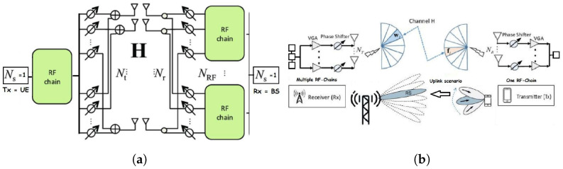 Figure 1
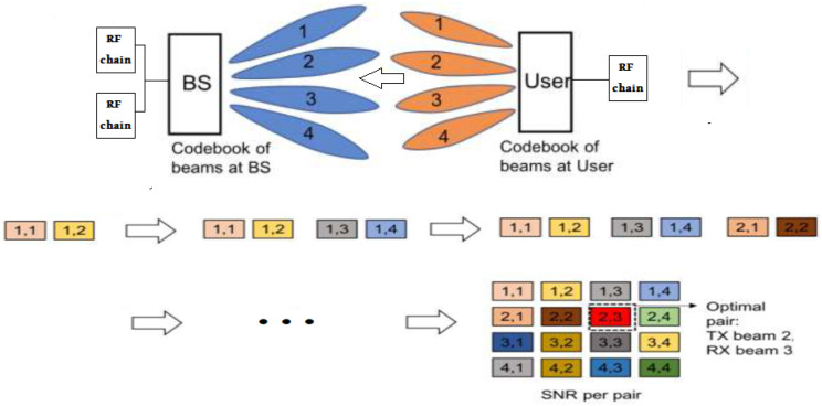 Figure 2
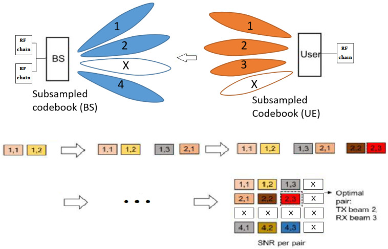 Figure 3
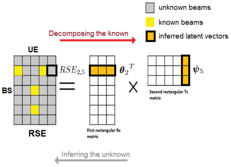 Figure 4
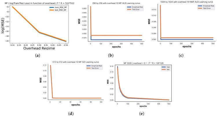 Figure 5
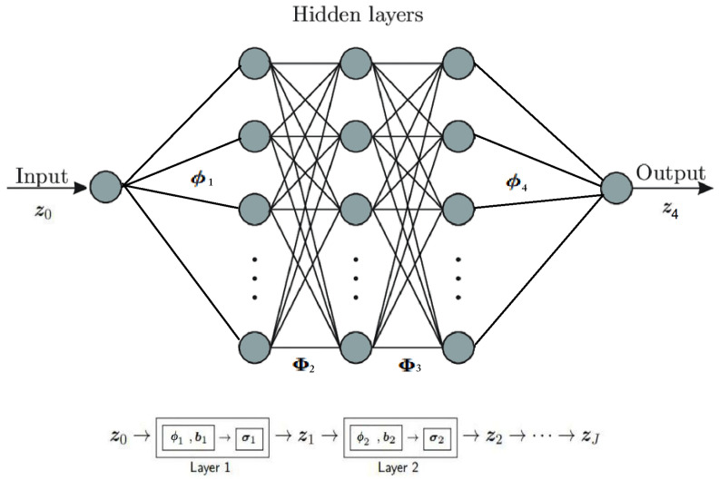 Figure 6
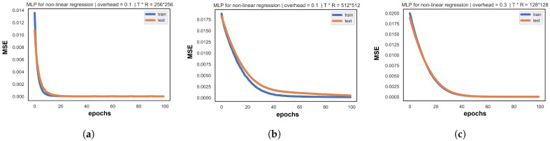 Figure 7
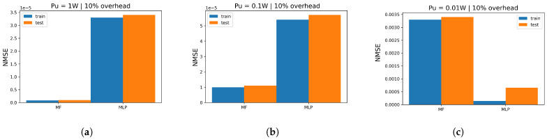 Figure 8
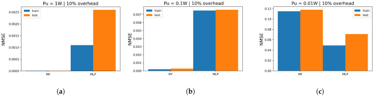 Figure 9
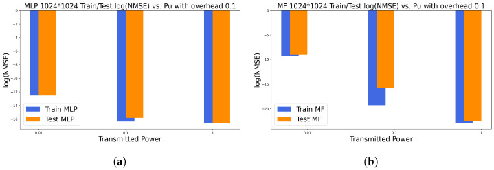 Figure 10
- —Télécom Paris, l’Institut Polytechnique de Paris, France
Peer Reviews
No public reviews on file for this paper yet. If you reviewed it on a platform where reviews are public (OpenReview, ICLR, NeurIPS, ICML), you can paste yours below so the community can read it here.
Videos
No videos yet. Explain this paper in a talk, walkthrough, or lecture? Add one.
Taxonomy
TopicsMillimeter-Wave Propagation and Modeling · Microwave Engineering and Waveguides · Radio Frequency Integrated Circuit Design
1. Introduction
Driven by the explosive growth trend of large-scale connectivity and higher data rate systems, wireless data traffic is expected to exponentially increase, growing to 5 zettabytes per month and reaching a 100 Gps data rate by 2030 [1] Thus, the latency in the 6th Generation is predicted to reach 0.1 ms, representing of latency, in order to support new emerging technical needs, including holographic images, Internet of Things applications, and autonomous driving.
Beam Alignment is frequently defined in the literature as beam sounding, i.e., beam training. It illustrates a fundamental problem in millimeter-wave Multiple Input, Multiple Output systems, defined as the exchange of information between the user equipment and the base station in order to accurately select the optimal beam-steering direction. The process of aligning the beams is related to several technical problems, such as beam forming, beam sweeping, beam tracking, and beam selection. The whole framework that unites these operations between and is often denoted as the Beam Management. To fulfill the BA task, beam patterns stored in large codebooks are used at both and . In fact, pencil beams with directional gain are increasingly being used in several applications in order to alleviate the severe path-loss attenuation and increase capacity and data throughput. On the other hand, massive MIMO systems provide large gain in spectral and energy efficiencies compared with conventional MIMO systems. Using mmWave technology, these systems mainly offer a better communication quality by increasing the system bandwidth and reducing the effects of noise and interference. Due to the diversification of future and towards applications and intelligent systems, scientists predict the continuous generation of massive datasets for deep processing through large bandwidths, which introduces mmWave bands as the golden spectrum band candidates. However, the limitations of mmWave communication physical properties of the channel are crucial: scattering, attenuation, low coherence time related to the Doppler effect, penetration loss, environmental constraints, and complex channel modeling in realistic urban scenarios. The major problem we aim to encounter in this paper is the inevitable high signaling/training overhead. For this reason, the main trade-off is to browse the most accurate and the least complex algorithm that optimizes finding the optimal beam pair based on sounded instantaneous Received Signal Energies and using the minimum (possible) amount of training samples.
Contributions: In this current work, we propose ML-based BA methods, for a single user massive mmWave MIMO, Uplink, with a wide-band channel. We assume a single radio frequency chain with large codebooks of possible analog beams at BS (also known as BS codebook) and UE (also known as UE codebook). We define a beam pair as one beam from the BS and UE codebook. By approximating the SNR with the Receive Signal Energy (RSE), we bypass the need for CSI, i.e., a blind approach. We sub-sample large codebooks into smaller sub-sampled BS and UE codebooks, and sound the beam pairs from the sub-sampled codebooks to generate the training set—a novelty of the approach. Using the RSE of the sounded beam pairs (sub-sampled codebooks), we propose to train the following ML methods to predict the RSE of the beam pairs that were not sounded: Matrix Factorization (MF), non-negative Matrix Factorization (NMF), and feed-forward (shallow) Multi-Layer Perceptron (MLP).
- We formulate the MF and NMF problems. We propose to use Block Coordinate Descent (BCD) and Block Gradient Descent (BGD) methods to solve each problem. We derive in depth all the update equations for these methods. We show that the BCD method converges to a stationary point from both MF and NMF problems. Our extensive numerical results show that, sub-sampling of the BS/UE codebooks, the remaining RSE values can be predicted extremely well (with a training/test error ) for every antenna configuration.
- We develop at length the equations of a general MLP model, the resulting loss function, and the corresponding optimization problem. In addition, we derive the equations of back-propagation for the MLP in question. Using extensive numerical results, we observe that sounding of original codebooks is sufficient to predict the RSE of the beam pairs that were not sounded, with negligible training/test error.
- We numerically compare the training/test losses of all the proposed models for a varying cardinality of codebooks and transmit powers. These results suggest that the BCD method for MF/NMF outperforms the MLP in terms of training and test error. Meanwhile, BCD for MF/NMF has a large computational complexity and the MLP exhibits medium complexity.
- Interestingly, by sounding of the BS/UE codebooks, the proposed ML models can predict the unknown RSE (beam pairs not sounded) with a negligible test error. Thus, the proposed methods achieve a reduction in pilot signaling overhead, compared with the SotA benchmark, without any noticeable loss in performance.
Notations: Matrices and vectors are respectively written in boldface upper-case and lower-case letters. We use for the trace, transpose, inverse, conjugate transpose, determinant, and Frobenius norm of a matrix and the identity matrix. is used to denote the (i, j)th entry of a matrix . We denote the Hadamard product by ∘, while illustrates a Euclidean projection of on and is applied element by element on . We denote the absolute value of x and as the entry t of a vector .
Methods/Experiment: The proposed approach is data driven and model based. The dataset is generated following the Saleh Valenzuela wide-band mmWave system model. It is based on Received Signal Energies for each and every beam pair in the massive MIMO Uplink setup stored in separate .csv files. The model-based solution to the empirical risk minimization includes deriving a closed-form solution to the formulated non-convex optimization problem, stating the theoretical guarantees of convergence and empirically illustrating the success of the proposed partial and blind Beam Alignment procedure using different algorithms. All simulations are executed on Infres GPU servers and the Comelec laboratory PC at Télécom Paris, having the following characteristics: Intel(R) Core(TM) i5-8365U CPU @ 1.60 GHz, 16 Go (RAM), x64 processor, and 64-bit operating system under the license of Windows 10 Enterprise LTSC 2018, version 1809. The manufacturer is Dell and is located in Paris, France. All python packages used in this work (numpy, scipy, keras, pytorch, matplolib..) are related to python 3.9 release. In fact, the experimental protocol is based on offline grid-search cross-validation, which requires GPU processing for the selection of optimal hyperparameters and online training/prediction for Matrix Factorization, non-negative Matrix Factorization, and Multi-Layer Perceptron. The comparison is conducted following a Quality of Service-based approach, simulating a variety of MIMO configurations and architectural setups, investigating the impact of varying the Received Signal Energy regime and empirically stating intersections and differences in the impact of the transmit power on model behaviors, loss values, optimal signaling overhead ratio, and optimal hyperparameters.
- Problem Statement: The main challenge addressed in this study is the high signaling overhead in Beam Alignment for mmWave MIMO systems, which hampers the efficient selection of optimal beam-steering directions.
- Research Questions and Hypotheses: This study investigates whether machine learning methods can effectively reduce the signaling overhead required for accurate beam-pair prediction in mmWave MIMO systems.
- Objectives and Aims: The primary objective is to develop and evaluate ML-based BA methods that minimize the training overhead while maintaining high accuracy in predicting the RSE for unsounded beam pairs.
- Significance and Rationale: The study proposes a novel approach to BA using ML techniques, which can lead to a substantial reduction in pilot signaling overhead and enhance the efficiency of future wireless communication systems.
2. Literature Survey
In conventional standards, Exhaustive BA, also called Brute Force BA, is the de facto approach for the alignment process. It is based on sounding all available beams at both and codebooks in order to exhaustively select the optimal beam pair. One obvious drawback is the fact that the resulting signaling overhead scales as the product of the and codebook sizes. At 60 GHz, the Exhaustive BA has been adopted in several mmWave or communication technologies, e.g., IEEE 802.15.3c [2] and IEEE 802.11ad [3]. It is conventionally applied in small MIMO configurations using small codebook sizes (e.g., codebooks of size for ) and guarantees optimal performance. For cellular networks [4], V2X communications, Unmanned Aerial Vehicles, or High-Speed Train applications, the infeasibility of brute-force-based BA pushes scientists to reduce the large signaling overhead from using massive antennas systems. State-of-the-art methods can be divided into two categories: classic BA and learning-based BA. Traditional techniques tend to use a more and more structured Beam Alignment design such as hierarchical multi-level codebooks [5] (training beamforming vectors are constructed with different beam widths at different levels) and an overlapped beam pattern [6], where the main idea is to augment the amount of information carried by each channel measurement, reducing the required channel estimation time and beam coding [7], where we assign a unique code signature to each beam angle in addition to subspace estimation/decomposition-based [8]. Compressed sensing-based algorithms [9] are also used in this context, taking advantage of channel sparsity. Therefore, we state two intersections in classic methods: they generally rely on exchange and Exhaustive BA. In contrast, lately, Machine Learning ( )-based BA has emerged and is continuously leading to some promising results. For instance, statistical models such as Kolmogorov model-based BA in [10] with sub-sampled codebooks reduce the signaling overhead: of Exhaustive provides accurate predictions for optimal beams at and in a partial procedure, similar to our approach. Deep learning through shallow neural networks is increasingly used by Wireless Communication scientists, where we distinguish two major paradigms: first, the ML methods related to Supervised Learning ( ) via a Support Vector Machine and Multi-Layer Perceptrons for joint analog beam selection in [11], convolutional neural networks for beam management in sub-6 GHz in [12] and for calibrated beam training in [13], recurrent neural networks such as Long Short-Term Memory network for beam tracking in [14,15,16], auto-encoders for beam management in [17], and several other neural architectures, and second, Reinforcement Learning ( ) in [18,19,20], generally used to resolve the problems of Multi-Armed Bandit and Markov decision process. In addition, neural architectures have the ability to extract features from the hidden interactions between and , providing fast and accurate estimations through different MIMO setups and channel realizations, especially when applied to massive datasets where more and more data/train samples are embedded. This work is an extension of [21]. In this paper, we extend the channel model to wide-band and we add multiple RF-chains at in a fully analog low-complexity architecture, where we investigate more tools for partial and blind . This paper is one of the first attempts to apply models and shallow Multi-Layer Perceptrons to a blind and partial Beam Alignment for massive mmWave SU-MIMO. Our work in [22] is related to the same approach and objectives, where we quantize the output of each RF-chain.
3. System Model
In this section, we illustrate the mmWave MIMO point-to-point system model. We consider an Uplink transmission from multiple-antenna user equipment using a single radio frequency chain and a multiple-antenna base station using multiple radio frequency chains. The proposed methods are performed at the , which has higher computational resources than . Figure 1a,b provide a diagram representation of the proposed architecture. and are respectively equipped with Uniform Linear Arrays of and antenna. We propose a low-cost/complexity fully analog architecture where has one radio frequency chain and has radio frequency chains. selects its analog beamformer from a codebook of feasible beam choices, , where is the corresponding index set. Moreover, selects its analog combiner from a codebook with as the index set of the codebook. We denote with the number of possible beamforming vectors at , i.e., the size/cardinality of the codebook, and , and the size/cardinality of the codebook, . Both beamforming and combining are fully performed in the analog domain using phase shifters at and ; thus, they satisfy the following constant modulus constraints, :
For our proposed approach, is responsible for receiving signal energies, denoted as , in order to learn their patterns and features for the purpose of accurately predicting the optimal beam indexes from their corresponding codebooks and send them to . We adopt the wide-band channel model given by
where represents the number of sub-carriers over the whole bandwidth through an scenario, k is the index of the sub-carrier k, and is the narrow band channel model representing the time domain channel impulse response with L-tapped delays given by , where L is number of paths (rank) of the channel; and are the angles of arrival at and the angles of departure from , noting AoA/AoD to correspond to the path (and both assumed to be uniform over ); is the complex gain of the path such that ; and last but not least, and are the array response vectors at both and , respectively. We further assume that the channel is completely unknown to both and . Henceforth, in this paper, we shall denote the beam pair as the combination of the beamformer indexed u from the codebook and combiner indexed i in the codebook . The signal at resulting from applying the beam pair , is expressed as
where is the transmitted pilot symbol associated with (having power ) and is the effective additive white Gaussian noise with unit variance ( ). We define the received Signal-to-Noise Ratio ( ) for the beam pair as . We assume a fully blind approach; i.e., neither nor has any knowledge of . Thus, computing the above expression is not feasible due to the fact that BS is assumed not to know . Thus, in this work, we will approximate the of the beam pair using the corresponding instantaneous Received Signal Energies ( ) expressed as . In other words, we will assume that for each beam pair .
Benchmark: Exhaustive : The de facto method for Beam Alignment is Exhaustive . It is accomplished by exhaustively sounding, jointly, the beams of both and codebooks, recording all entries of , and exhaustively searching for the indexes of the beam pair that maximize at , i.e, . Thus, the matrix is computed/recorded -entries, with each of pilot symbol, since samples are simultaneously received at the for every pilot transmission (see Figure 2). Consequently, the pilot signaling overhead of the Exhaustive is , which implies that the overhead of this benchmark scales poorly with the and codebooks.
Proposed partial Beam Alignment using sub-sampled codebooks: Recall the designation of the beam pair as the beamforming vector of the index u in the codebook of beams and the combining vector of the index i in the codebook of beams. First, we select (at random) the indexes of the sub-sampled codebooks of beams at and , and , such that and , and . The idea behind this approach is to only sound beam pairs from the sub-sampled codebook of beams, and . We thus define the training set, , as the sub-sampled codebook indexes at and , i.e., . Then, the of the sounded beam pairs (training set) is given to several ML methods, and the learned ML model is used to predict the of non-sounded beam pairs.
We formalize this proposed method below. We express both the received signal and for the beam pair resulting from the sounded beam pairs (i.e., training set), as follows:
The dataset is formulated using the following incomplete matrix, :
where denotes the element of , . Evidently, the value of is undefined for the beam pairs that were not sounded, designated as unknown-RSE matrix coefficient. Those are the missing entries, which are predicted using one of the following proposed methods: (i) low-rank and (ii) shallow (feed-forward) , where we utilize the sounded entries as the training set, . Then the training set, , is fed into one of the above ML models, which will predict the of non-sounded coefficients in , denoted as ‘Unknown’, in (5) (see Figure 3). Finally, the pilot signaling overhead for the above-proposed sub-sampled codebook method is . We split the RSE dataset into a training set and a test set such that . In this paper, denotes the true value (label) of the RSE for the beam pair in the training set , and denotes the true value (label) of the RSE for the beam pair in the test set .
Signaling overhead ratio: It is defined as , where and are, respectively, the sizes of the and sub-sampled codebooks used in our proposed partial beam sounding, while and refer to the original size of the codebooks, and measures the signaling overhead of all the proposed , , and methods compared with that of Exhaustive . Evidently, a small value for is desired to reduce the signaling overhead of our proposed method. However, a low implies that the size of the training set is small. As a result, the proposed method will not be able to extract enough data patterns due to the (too) small number of training samples, resulting in a larger prediction error. As one of the contributions of this work, we will (empirically) find as small a value for as possible while still having extremely small training and prediction error.
Conjecture: Note that, from the equations of the narrow-band channel model and the wide-band channel model , it is simple to verify that and . Assume that . Thus, we can approximate the RSE matrix as
If , then it can be shown that the RSE matrix is such that . This implies that if , then is a low-rank matrix, i.e., .
While the proof for this necessary condition eludes the authors, we empirically observed that if is large, then the number of non-zero singular values of , , satisfies the above upper bound, i.e., .
Remark 1. Recall the expression for the effective rate, r, , where Ω is the pilot signaling overhead and is the number of symbols per block. Thus, the problem of maximizing r is written as the following series of equivalent problems:* , where the last* ⇔ is due to the fact that the is a strictly monotonically increasing function in x. This result implies finding the optimal beam pair that maximizes r is equivalent to finding the best beam pair that maximizes the .
Remark 2. The information (number of entries) needed to represent the matrix is measured as . This result is evident from performing the on and counting the resulting number of entries. Thus, if is severely rank deficient, i.e., extremely compressible, then methods such as will exhibit extremely small training and test error. Conversely, if is full rank, i.e., not compressible, then the training and test of will be quite large.
4. Matrix Factorization and Non-Negative Matrix Factorization
4.1. MF and NMF Problem Formulation
The intuition behind low-rank is to model the of the sounded beam pairs (i.e., entries of that are known as ) as an inner product between two D-dimensional latent vectors/factors, , as illustrated in Figure 4. Specifically, the of the beam pair , denoted as , is modeled as , , where D is the size/dimension/complexity of the Matrix Factorization model latent factors and are the model parameters (to be optimized). In addition, due to the low-rank model, D is assumed to be much smaller than the dimensions of , i.e., . The of the beam pair is known from sounding the sub-sampled codebooks (i.e., label). The general formulation of our loss function describes the distance between the true value and the predicted value , which corresponds to the output/prediction: . The Empirical Risk (also known as training error) is defined as the average across all the individual loss function . We define the regularized Empirical Risk function as the above empirical risk in addition to the following regularization terms:
where is the set of regularization hyperparameters used to balance the model, preventing any overfitting or underfitting. The Empirical Risk Minimization corresponding to the model is given by
For the Matrix Factorization variant , the optimization problem is given by
where denotes the optimal latent vectors for MF and NMF. The test loss (also knows as test error) is given by applying the general loss on the unknown data samples (non-sounded beams) using optimal parameters and : , where is the test set of our learning model.
4.2. Solutions for MF
We resolve the problem using the following methods: (i) Block Coordinate Descent (BCD) often denoted as Alternating Least Squares (ALSs), (ii) BCD with Stochastic Gradient Descent, and (iii) Block Gradient Descent (BGD), which merges BCD and Gradient Descent (GD) definitions.
BCD for MF (BCD MF): BCD proceeds by splitting the optimizing problem into sub-problems, supposing that all other blocks are known/fixed. We will show that each sub-problem is strongly convex in each block, and the BCD algorithm converges to a stationary point. The application of BCD to the problem results in two sub-problems, S1 and S2, which are solved iteratively. At iteration k, the sub-problem is defined by fixing the block and the update/solve block only, as follows:
Moreover, the sub-problem is defined by fixing the block in and the update/solve block , only, as follows:
We will rewrite into as series of equivalent problems as follows:
where is the set of row indexes u in the RSE matrix corresponding to the column i in the known entries of the RSE matrix, and . We derive the closed-form solution for the sub-problem S1 by finding the global min of , as follows:
Similarly, we rewrite the sub-problem (S2) into the following series of equivalent problems by stating the last one:
where is the set of column indexes i in the RSE matrix corresponding to the row u in the known entries of the RSE matrix, and . Next, we derive a closed-form solution for the sub-problem S2 by finding the global min of , as follows:
Thus, BCD updates to solve MF are given as follows:
where ^(k)^ represents the index of the BCD iterations, (u,i) are the codebook indexes at and , and denotes the of the (u,i) beam couple. The solution is reached after the interval/gap between consecutive iterations reaches a predefined or a max number of iterations, . We have the following result.
Corollary 1. The sequence of updates generated by BCD, in (8), is non-increasing (in k) and converges to a stationary point as .
Proof. See Appendix A. □
Block Stochastic Gradient Descent (BSGD) for MF (SGD MF): SGD MF proceeds by taking T plain SGD steps (mini-batch size ). BGD proceeds by taking T SGD steps for each block BCD. We first choose at random a single training sample . The BSGD update for the sub-problem (S1) is done by performing SGD for , i.e., choosing at random a single index and computing the plain SGD , where u is a random index from , and is the plain SGD on . The corresponding update is given as
where u is a single index chosen at random from , , , ^(k)^ is the iteration index for SGD, and is the plain SGD over one random sample . Similarly, the update for the sub-problem (S2) is done by taking T plain SGD steps of , i.e., the SGD, , where i is single random index from . Thus, the SGD MF update for the sub-problem (S2) is expressed as
where i is a single index chosen randomly from , , , and is the plain SGD gradient computed with one sample , chosen at random. We write the SGD MF updates as
where u is a random index chosen from , and i a random index from . is the step size for SGD.
BGD for MF (BGD MF): Rather than having a closed-form solution for each optimization block, BGD proceeds by taking T gradient steps for each block T gradient step. We skip the details here for space limitations. Thus, the BGD updates for the problem are expressed as
where (u,i) are the codebook indexes at and , k is the GD iteration index, and is the BGD step size ( ).
4.3. Solutions for NMF
Our proposed follows the exact steps as in , with the main difference of constraining the latent vectors being non-negative . Likewise, we solve the problem, , using BCD, SGD, and BGD.
BCD for NMF (BCD NMF): The derivations of BCD for (11) are identical to those of BCD for (8), followed by the corresponding projection operation. The updates of BCD for derivations are given by
where ^(k)^ is the BCD iteration index, and is applied element by element on , i.e., a Euclidean projection of on . Since the projection is Euclidean (non-expansive operator), the corollary stated in the previous subsection applies to the BCD for too.
Block Stochastic Gradient Descent (BSGD) for NMF (SGD NMF): The SGD NMF derivations are exactly the same as that of SGD MF, followed by a projection . We thus express the SGD NMF updates as
where u is a random index chosen from , i is a random index from , , and is the SGD step size ( ).
BGD for NMF (BGD NMF): The solution and derivations for BGD NMF are the same as those for BGD MF, followed by a projection , i.e,
where , ^(k)^ is the GD iteration index and is the GD step size ( ). We use a constant step size for all these methods.
4.4. Prediction for MF and NMF
For both and , the predicted of the beam-pair , for beam indexes that were not sounded, is expressed as
where is the test set and are optimal solutions to MF (or NMF). Afterwards, we search for the optimal beam pair at and as the one with the highest value over both training and test sets, as follows:
4.5. Proposed BA Algorithm Using MF/NMF
Due to the fact that the updates given in a closed-form solution, we can quantify the computational complexity of all of the above methods. As seen from the updates for BCD MF and BCD NMF, we have to invert two matrices (for the sum problems S1 and S2). Thus, the (per-iteration) computational complexity of BCD MF and BCD NMF is approximated as . Moreover, for BGD MF and BGD NMF, one has to compute two full-batch gradients over all training samples in (for the sub-problems S1 and S2). Consequently, the complexity, per-iteration, for BGD MF and BGD NMF is approximated as . Finally, for SGD MF and SGD NMF, since we use a mini-batch size (for the sub-problems S1 and S2), the resulting per-iteration computational complexity is approximated as . Solving the and problem, we employ methods such as BCD, BGD, or SGD. All details are shown in Algorithm 1. Algorithm 1 Proposed MF/NMF-Based BA Method.
-
Input: , , ,
-
-Generate randomly sub-sampled codebooks, , satisfying
-
-Sound beam pairs from training set, .
-
-Record corresponding in and generate mat. , in (5)
-
-Select model: MF or NMF
-
-IF MF model selected
-
solve with BCD for MF, in (8) or solve with BGD for MF, in (10) or solve with SGD for MF, in (9). At the end of training, return optimal latent vectors,
-
-IF NMF model selected
-
solve with BCD for NMF, in (11) or solve with BGD for NMF, in (13) or solve with SGD for NMF, in (12). At the end of training, return ideal latent vectors,
-
-Use ideal latent vectors , to predict unknown of test set, , in (14)
-
-Search training and test sets, for beam pair w/ largest , (15)
-
Output: ,
While, for MF BCD and NMF BCD, the only hyperparameter is the model size D, MF BGD and NMF BGD require, in addition to D, , the GD step size as hyperparameters.
4.6. Numerical Simulations
This section illustrates our numerical setup. The number of antennas at and , 256, 512, . We set up and . The overhead ratio regime 0.7 0.5 0.3 0.1}. The number of sub-carriers and the number of channel paths L is 2. We vary the transmitted power, . We use codebooks at and . The optimal hyperparameters are chosen to minimize test loss. The model dimension , the learning rate , and the regularization factors . For each MIMO configuration and for each regime, we randomly generate and store the resulting matrices.
We propose to investigating six models in total (BCD MF, BCD NMF, BGD MF, BGD NMF, SGD MF, SGD NMF) with respect to three transmitted power regimes: high , medium W, and low W with fixed . In Table 1, we provide a summary for all proposed system parameters. We use the training Normalized MSE ( ) to evaluate the training error, expressed as . We also define . The range of training error and the overall behavior of -based models are different and distinctive from models in both and ; for instance, -based models’ error range are around , while -based models are around . Thus, is more accurate. However, converges faster and the cost function drops to low values from the very first iterations. In addition, for and , the train decreases with the increase in the overhead ratio , as seen in Figure 5. Low and medium regimes are characterized by noisy links between and and represent a more challenging experimental environment. -based models tend to be faster in reaching low error values, while -based models are more accurate. (For instance, generally ameliorates the quality of prediction compared with ).
Regarding simulation figures, Figure 5a states the decrease of train/test in function of the overhead ratio (more training samples result in fewer errors); Figure 5b,c track the instant drop in loss values from the very first iterations for -based models; and Figure 5d,e present the progressive convergence of cost function among the iterations when we use -based models. In summary, Table 2 outlines the optimal (minimum) signaling overhead ratio required for the all proposed system configurations, the optimal model (holding the smallest total cost function), the related combination of optimal hyperparameters, and the corresponding train/test error values. When the signal is affected with much noise, it is harder to keep the same range of error when compared with high a regime. In fact, models keep the same (minimum) signaling overhead ( ) regardless of the transmitted power regime, being able to accurately predict with just of sounded beams. Thus, the proposed methods are able to reduce the pilot signaling overhead by compared with Exhaustive with negligible training and test errors.
5. Multi-Layer Perceptron
5.1. MLP Problem Formulation
We consider a feed-forward , with J layers, modeled as a composition of J non-linear functions/layers. Let be the input, and be the output; see Figure 6. We denote with all the hidden layers. We assume for simplicity that the width of all the layers is the same, denoted as D, i.e., ; see Figure 6. The equation describing layer 1 is given by , where is the output of layer 1, is the resulting weight vector, and is the non-linear activation function for layer 1. We use one hot encoding for the MLP input , i.e., for all training samples, . We express the output of the hidden layers, , as , where is the input of the layer j and is its output ; is the weight matrix for the layer j ; and is the element-by-element non-linear activation function for the layer j, . Finally, the relation for the last layer is expressed as , where is the output for layer J, is its weight vector, and is the non-linear activation function for the layer J. We express the output of the MLP (as a function of all layers) as
The output of is made to fit/approximate all the values at all training samples; , . We define the MSE loss for the sample in the training set as the distance between the MLP output and the known RSE label for the beam pair , , i.e,
Then, the empirical risk is defined as the average of the individual loss across the training set , . The empirical risk minimization for the MLP is given in .
5.2. MLP Learning
We propose to learn the optimal weights via back-propagation (BP). We choose an arbitrary mini-batch of samples of size and define the mini-batch loss as
We express the partial derivative of the loss corresponding to the mini-batch with respect to each layer as
where
and ∘ denotes the Hadamard product. We express the BP weight update of the mini-batch loss , for all layers , as
where ^(k)^ is the BP iteration index, is the value of at iteration k, is the BP step size (learning rate) for the layer j at iteration k, and is the partial derivative given in (18) evaluated at .
Back-propagation algorithm with mini-batch
Choose the mini-batch as a random subset of the training set .
- Compute the loss function for all samples in the mini-batch in (17).
- Compute the partial derivative of the mini-batch loss with respect to in (18).
- Update the weights of each layer as in (19).
We assume that the BP learning rate is the same for all layers, .
5.3. Prediction Using MLP
The prediction for the sample (u,i) in the test set , using optimal weights , is as follows:
Therefore, the test is defined as
We then select the optimal indexes and related to the highest value, as follows:
5.4. Proposed BA Algorithm Using MLP
The Multi-Layer Perceptron-based Beam Alignment is specified in Algorithm 2. Algorithm 2 Proposed MLP-Based BA Method.
-
Input: , , ,
-
-Generate randomly sub-sampled codebooks, , satisfying
-
-Sound beam pairs from training set, .
-
-Record corresponding and generate mat. , in (5)
-
-Train weights (using back-propagation algorithm)
-
return optimal weights,
-
-Use optimal parameters , to predict unknown of test set, , in (21)
-
-Search training and test sets, for optimal beam pair , holding the largest , (22)
-
Output: ,
We assume that the number of neurons per layer D, the number of layers J, the mini-batch size , and the BP learning rate are hyperparameters. They are tuned using a grid search cross-validation.
5.5. Numerical Simulations
We define the training and test cost functions as follows:
Therefore, we used the same system configurations as for , resumed in Table 1. Moreover, we choose the learning rate , , , , while the batch size , 4, 8, 16, 32, 64, , the number of hidden layers . For each layer, the number of neurons , 16, 32, 64, . We use the Rectified Linear Units as our activation function for all layers.
Similar to , train performance is observed when we track the evolution of the cost function , applied to the training samples of the set , in a function of iterations. The range of considerably low-error values and the overall learning behavior of the architecture illustrates that our shallow neural network successfully resolves the non-linear regression problems related to our BA process. For massive setups, reaches around error in a high regime. However, this cost value increases as long as the amount of noise and interference augments. Note that the train also decreases when we increase the size of the dataset matrix , which provides more samples for to improve the feature extraction and the prediction quality. Regarding the unknown beams, test error values in the numerical result tables are close to the train cost (with no overfitting or underfitting in the corresponding learning curves). Moreover, the test loss is impacted by the transmitted power regime the same way as the training process. Identical to -based , the learning curves in Figure 7 plot the same shape of curve with a continuous monotonic decrease in the train and test cost among the iterations: the convergence is progressive among the iterations, and at the last epoch, training and test values land at considerably low error values and prove that accurately fits to our problem and provides a concrete solution for -based . From a perspective, Table 3 resumes the smallest (optimal) signaling overhead required for a successful beam sounding based on reliable prediction quality. Similar to , for all the proposed transmitted power, requires of the total beam pairs to fulfill the matrix.
6. Results and Discussion
6.1. Train/Test Prediction Performance Comparison
For the six -based models, we select the best one (minimum test error) to represent the family of methods in this section and compare it with . When we analyze (Table 1 and Table 2), we notice that the transmitted power regime impacts the quality of prediction by reducing the overall loss. For , we observe that the loss damage is large. We jump from around for massive configurations (256, 512, and 1024) to for smaller setups. For , we spot the increase in the overall loss when we decrease . Thus, seems to be the most robust architecture with respect to changing the transmitted power. Additionally, we empirically notice that the change in the values does not impact the optimal hyperparameters selected from cross-validation. Furthermore, when we track the evolution of the training/test cost in the function of iterations, we observe balanced models with no signs of overfitting or underfitting. On the other hand, when the transmitted power decreases, tend to be the most impacted models in terms of train/test error, while the error is robust.
On the other hand, from a perspective, concerning the evolution of the optimal (minimum) required signaling overhead and what impact can the regime have on the optimal required values, in reference to Table 1 and Table 2, all the proposed models required just of the total number of beam pairs at and for all antenna configurations from to for all the proposed values. This proves that the transmitted power impacts the quality of prediction but not the number of beam pairs required for training. In fact, low leads to damaging the signal quality and subsequently damages the quantity of useful information to be extracted from the datasets. Finally, the only cases where the regime impacts the optimal overhead ratio is among the smallest configurations, for instance, the setup where it seems normal for all learning models to demand more data to learn from (more hidden interactions between and as features to extract). These are the experimental situations where Exhaustive is technically feasible.
6.2. Similarities and Differences between Models
All models required just of the beams for training for all the proposed massive setups. Moreover, all the proposed models are shallow neural architectures with few hidden layers for low-complexity constraints. Even among the largest configurations, the optimal dimensions of models picked from the cross-validation illustrate small networks with no need to require dense architectures. Furthermore, all models succeeded with the matrix completion task, and they all illustrate a monotonic decrease in loss values as long as we increase the MIMO setup. Additionally, -based models are the most accurate reaching loss values in the range for massive setups in a high regime, and their cross-validation illustrates smaller grid search where there are fewer hyperparameters to tune. However, they are the slowest models when applied to high-dimensional MIMO setups. On the other hand, illustrates a good balance between run time (complexity) and loss values (prediction quality). It reaches around and loss for massive configurations. In addition, the is the most robust model facing the changes in the values. In Figure 8, for , the figure illustrates the train/test in the function of each model and the corresponding transmitted power: in Figure 8a, for , achieves its best performance, slightly better than with the difference between achieved cost values at around . In Figure 8b, when , still gets the best performance, marginally better than with an value difference of around . In Figure 8c, when , noticeably gets impacted (overall loss around ) while provides the best prediction performance: this suggests that when is small, is more robust than , which performs best in high regime. Similarly, almost same remarks hold for Figure 9 when we simulate the configuration: in Figure 9a, reaches considerably better performance compared with with . In Figure 9b, kept the same range of error, which states again the robustness of the model while got severely impacted ( ) but sill holds the best performance. In Figure 9c, when is weak, illustrates the worst performance in all simulations. On the other hand, got slightly impacted with an overall loss of and reaches the best quality of prediction. In Figure 10, we investigate the highest configuration . Similar conclusions for Figure 8 and Figure 9 hold for this figure in terms of best model ( for , and for ). In addition, we aim to investigate the overall impact of varying the transmitted power. Thus, we track the values while switching from one regime to another: In Figure 10, in Figure 10a, for , the curve gap from low/medium is . The gap in the medium/high regimes is almost negligible ( ). Finally, in Figure 10b, the gap is around and : at each change of , is considerably impacted. To sum up, the choice of the optimal model strongly depends on the available complexity and the given transmitted power . In fact, , whether through or optimization, is the best model when the transmitted power is high ( ). In this case, converges faster but has higher complexity than . However, for are the slowest models to converge but show negligible complexity. On the other hand, if we aim to prioritize run time, exhibits the fastest predictions with good prediction error. Finally, it is wise to opt for if the system is to operate under various transmitted power regimes where offers good prediction quality for every value and the available complexity is medium.
7. Conclusions
In this paper, we proposed a blind Machine Learning-based Beam Alignment using Matrix Factorization, non-negative Matrix Factorization, and Multi-Layer Perceptron. We assumed an Uplink massive mmWave MIMO system using single RF-chains at and multiple RF-chains at though a fully analog architecture. The proposed approach consists in sounding the of sub-sampled codebooks at and . The of the non-sounded beams is predicted using , , and models. Our results show that, by sounding just of the total beam pair samples, we may predict with high accuracy the unknown values, which massively reduce the large signaling overhead of Exhaustive . Our future work investigates the scalability of our approach to a multi-user scenario. Robustness and -interpretability are other research directions for modeling industrial deployment.
The reference list from the paper itself. Each links out to its DOI / PubMed record.
- 1Wang Y. Wei Z. Feng Z. Beam Training and Tracking in Mm Wave Communication: A Surveyar Xiv 20222205.10169
- 2IEEE Std 802.15.3c-2009 IEEE Standard for Information Technology—Local and Metropolitan Area Networks—Specific requirements—Part 15.3: Amendment 2: Millimeter-Wave-Based Alternative Physical Layer Extension IEEE Piscataway, NJ, USA 2009
- 3IEEE Std 802.11ad-2012 IEEE Standard for Information technology—Telecommunications and Information Exchange between Systems—Local and Metropolitan Area Networks—Specific Requirements-Part 11: Wireless LAN Medium Access Control (MAC) and Physical Layer (PHY) Specifications Amendment 3: Enhancements for Very High Throughput in the 60 G Hz Band IEEE Piscataway, NJ, USA 2012
- 43GPP. TS 38.211 V 16.7.1 NR; Physical Channels and Modulation; ETSI Technical Specification 138 211 V 16.10.0; Released: 07/2022 Available online: https://www.etsi.org/deliver/etsi_ts/138200_138299/138211/16.10.00_60/ts_138211 v 161000 p.pdf(accessed on 9 July 2024)
- 5Noh S. Zoltowski M.D. Love D.J. Multi-Resolution Codebook and Adaptive Beamforming Sequence Design for Millimeter Wave Beam Alignment IEEE Trans. Wirel. Commun.2017165689570110.1109/TWC.2017.2713357 · doi ↗
- 6Kokshoorn M. Chen H. Wang P. Li Y. Vucetic B. Millimeter Wave MIMO Channel Estimation Using Overlapped Beam Patterns and Rate Adaptation IEEE Trans. Signal Process.20166560161610.1109/TSP.2016.2614488 · doi ↗
- 7Tsang Y.M. Poon A.S.Y. Addepalli S. Coding the Beams: Improving Beamforming Training in mm Wave Communication System Proceedings of the 2011 IEEE Global Telecommunications Conference—GLOBECOM 2011 Houston, TX, USA 5–9 December 20111610.1109/GLOCOM.2011.6134486 · doi ↗
- 8Buzzi S. D’Andrea C. Subspace Tracking and Least Squares Approaches to Channel Estimation in Millimeter Wave Multiuser MIMOIEEE Trans. Commun.2019676766678010.1109/TCOMM.2019.2924885 · doi ↗