Fractional Telegrapher’s Equation under Resetting: Non-Equilibrium Stationary States and First-Passage Times
Katarzyna Górska, Francisco J. Sevilla, Guillermo Chacón-Acosta, Trifce Sandev

TL;DR
This paper studies a fractional telegraph equation with resetting, revealing non-equilibrium states and optimal resetting rates for first-passage times.
Contribution
The paper introduces a novel approach to analyze fractional telegraph processes under resetting, revealing non-equilibrium stationary states and optimal resetting rates.
Findings
The system reaches non-equilibrium stationary states in the long-time limit due to resetting.
The mean squared displacement saturates as a result of the resetting mechanism.
An optimal resetting rate minimizes the mean first-passage time.
Abstract
We consider two different time fractional telegrapher’s equations under stochastic resetting. Using the integral decomposition method, we found the probability density functions and the mean squared displacements. In the long-time limit, the system approaches non-equilibrium stationary states, while the mean squared displacement saturates due to the resetting mechanism. We also obtain the fractional telegraph process as a subordinated telegraph process by introducing operational time such that the physical time is considered as a Lévy stable process whose characteristic function is the Lévy stable distribution. We also analyzed the survival probability for the first-passage time problem and found the optimal resetting rate for which the corresponding mean first-passage time is minimal.
Genes, proteins, chemicals, diseases, species, mutations and cell lines named across the full text — each resolved to its canonical identifier and authoritative record.
Click any figure to enlarge with its caption.
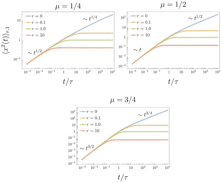 Figure 1
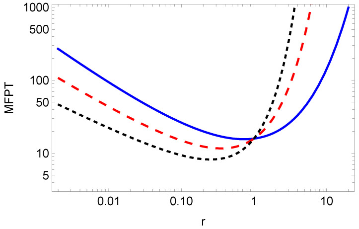 Figure 2
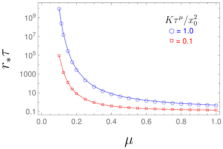 Figure 3
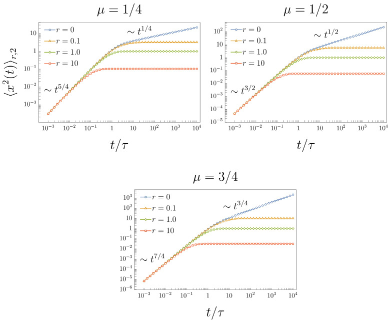 Figure 4
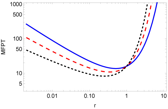 Figure 5
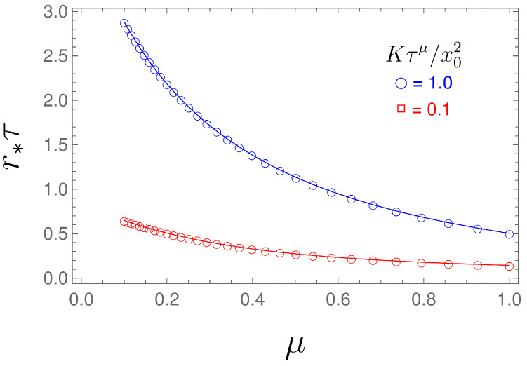 Figure 6
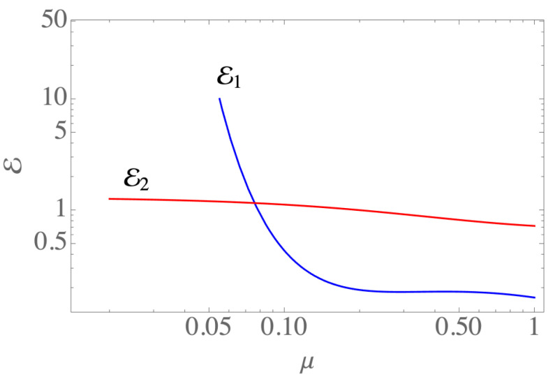 Figure 7
- —UNAM-PAPIIT
- —German Science Foundation
- —Alliance of International Science Organizations
- —Alexander von Humboldt Foundation
- —NCN Research
Peer Reviews
No public reviews on file for this paper yet. If you reviewed it on a platform where reviews are public (OpenReview, ICLR, NeurIPS, ICML), you can paste yours below so the community can read it here.
Videos
No videos yet. Explain this paper in a talk, walkthrough, or lecture? Add one.
Taxonomy
TopicsCensus and Population Estimation · Data Analysis and Archiving · Historical Psychiatry and Medical Practices
1. Introduction
Due to economic and military reasons in the XIX-th century, the rapid communication between the countries belonging to the British Empire was an important matter. To send a message from one part of the Empire to another was a true challenge, for its solution contributed to many famous physicists of that time, namely J. Maxwell, Lord Kelvin, and O. Heaviside. Nevertheless, only Heaviside solved this problem. He proposed the so-called telegrapher’s (telegraph) equation (TE) to describe the current propagation inside the telegrapher’s cable [1]. His equation is a hyperbolic equation which, in -dimensional space, has the following form
where is a time parameter measured in seconds, and v is the propagation velocity measured in seconds/meter. The boundary conditions are set to zero at infinity, while the initial conditions are
These boundary and initial conditions, allowed C. R. Cattaneo [2,3] and P. Vernotte [4] to employ Equation (1) to describe the heat transport. Thus, the physical interpretation of and v is changing. Here, modifies the Fourier law which connects the heat current and the temperature such that we have
The parameter v is associated with heat conductivity. Recently, Equation (1) has been used to characterize the diffusion process with finite propagation velocity v [5], where , K is the diffusion coefficient, and the Fourier law is replaced by Fick’s law. In this case, the solution of the telegrapher’s equation is a probability density distribution (PDF) and, for arbitrary initial conditions, is presented in Ref. [6] (Equation (102) on p. 303 and/or [7] Equation (7.4.28)). This solution for the initial conditions given by Equation (2) reduces to the form
derived in Ref. [8]. We use the standard notation for which denotes the Heaviside step function, and is the modified Bessel function of the first kind of order . The corresponding mean squared displacement (MSD) reads
which leads to the ballistic time dependence in the short-time regime and to the linear time dependence in the long-time one.
Equation (1) characterizes the telegraph process whose corresponding Langevin equation reads
where v denotes the constant particle speed, and is a stationary dichotomic Markov process that jumps between two states; , with a mean rate [9,10,11,12] ( , is a time scale that corresponds to the inverse mean sojourn time for each state). As shown in [13,14] subordinating this process by the Lévy process, we can find the fractional telegrapher’s equation of type I (abbreviated as FTE-I), namely
where and is the fractional derivative in the Caputo sense (see Appendix A). Equation (5) can be interpreted as an anomalous diffusion equation, which can be derived by using the continuity equation with an appropriate modified constitutive relation [15].
Despite the compelling generalization given by Equation (5), whose higher fractional derivative is always twice the lower one, it is possible to postulate different kinds of fractional telegrapher’s equations. For instance, we focus on one of these possibilities called type II (abbreviated as FTE-II), which has the form (this form corresponds to Equation (17) in Ref. [15])
where . In this case, the higher fractional derivative is always larger than 1. Equations (5) and (6) are completed with the same initial and boundary conditions (2) as for the telegrapher’s Equation (1). We can also find different fractional generalisations of the TE [5,10,15,16,17,18], including non-Markovian discrete time versions of the telegraph process [19], TE in random media [20,21,22], telegraph processes with random velocities [23], etc.
In this paper, we consider the stochastic resetting of the PDFs and that solve Equations (5) and (6), respectively. The stochastic dynamics of the particle, which are initially located at at , under the effects of stochastic resetting, are described by the renewal equation [24]
where , indicates the probability density corresponding to the different telegrapher’s equations considered here; is the probability that no renewal has taken place up to time t. We consider here the stochastic Poissonian resetting with probability and from this, we have , where r is the resetting rate. The renewal Equation (7) for Poissonian resetting has the form [24,25,26]:
which, in the Laplace space, reads
Furthermore, we assume that the particle is instantaneously reset to the initial position. These assumptions offer the possibility of analytical calculations, as well a description of the experimental results for the mean-first passage time under stochastic resetting, by using holographic optical tweezers [27] or laser traps [28].
The paper is organized as follows. In Section 2, we consider the stochastic resetting of FTE-I. For that purpose, we find its solution in two ways based on integral decomposition techniques. This decomposition is rooted in recognizing the Brownian motion or the telegraph process. Next, we will reset the process described by FTE-I and calculate the first-passage time problem and survival probability. In Section 3, we repeat all procedures with the stochastic resetting for FTE-II. The paper is summarized in Section 4. The paper contains four Appendices.
2. FTE-I under Resetting
The PDF can be found in two ways, which come from the Efros theorem (Appendix C) applied to . In the Laplace–Fourier (LF) space, it is written as
Here,
and and are the Laplace and Fourier coordinates, respectively. The Efros theorem allows us to make the integral decomposition of Equation (10), for which we represent as the integral with the Gaussian
and
The function for is non-negative, such that it can be named the PDF of the leading process. Another possibility is to present as the solution of the telegrapher’s equation given by Equation (3) and being for the PDF of the leading process (for details, see Section 2.2). Hence, the solution obtained in this way is called the subordination approach. Both techniques in the presence of stochastic resetting will be described below, and we show that they lead to the same results.
2.1. Resetting of FTE-I—The First Possibility
Let us begin by examining the outcomes that can be derived from the second equality in Equation (10). In the short-time regime, , we have that Equation (10) is approximated by
which, after inverting the Laplace and Fourier transforms, we obtain the fractional wave equation (fWE)
Transport in this regime is described by the fWE. In the opposite regime, i.e., in the long-time regime, , Equation (10) is asymptotically approximated by
which corresponds to the standard fractional diffusion equation (fDE) after inverting the Laplace and Fourier transforms, i.e.,
In the general case, upon performing the Fourier transform inversion of Equation (10), we can express it in Laplace space as:
which, after taking the inverse Laplace transform, can be written in t-space as the generalized diffusion equation
The series representation of the two-parameter Mittag–Leffler function is given by Equation (A1) for . After multiplying the last equation by and integrating over space we are led to first-order differential equations for the MSD, which can be integrated straightforwardly to give . We emphasize that the procedure of expressing the hyperbolic-like Equation (5) as the parabolic-like Equation (19) is only formal and it is possible only for the diffusion-like initial conditions (2). Formally, we can present the solution of Equation (19) as
where and are given by Equations (12) and (13), respectively. The same results can be obtained using Equation (A3) resulting from the Efros theorem in which , , and . In the LF space, it figures as
Note that is a non-negative function for . That comes from the Bernstein theorem [29] and the fact that , for this range of , is a completely monotonic function (CMF), i.e., the non-negative function whose derivatives exist and alternate, see Appendix B. In consequence, we can say that , given by Equation (20) for is a PDF expressed by the subordination approach, in which the leading process, described by , subordinates the parent process characterized by the normal distribution [13,14]. The function for is not a CMF. Then, according to the Bernstein theorem, is negative or contains negative parts. However, calculated from Equation (21) for is a CMF, yielding that its inverse is non-negative and can be called a PDF.
The corresponding MSD can be expressed in terms of the MSD of the normal distribution , we have
from where, by inverse Laplace transform, one finds
which is a known result [5]. From (22), we have that in the short-time regime, and in the long-time regime; see Figure 1, curves marked with circle symbols for , 1/2, and 3/4.
If we reset to the initial position according to the stochastic Poissonian resetting , where r is the resetting rate, then the corresponding follows the renewal Equation (8) for . In Laplace space, it reads Equation (9) for , which, after employing Equation (21), gives
From here, we conclude that in the long-time limit, the system approaches the non-equilibrium stationary state (NESS) , which is explicitly given by
The NESS is given by the Laplace distribution with a stationary variance around the average value . For , the NESS is analogous to Equation (27) of Ref. [8]. For , we recover the result for the NESS for an anomalous diffusion process under resetting [24,30,31,32,33], i.e., . We want to point out the exponential decay of the NESS tails, which is a characteristic induced by the stochastic Poissonian resetting process.
For the MSD in the case of resetting, we have
from which we obtain
In the short-time limit it behaves as , and in the long-time limit it approaches the constant value,
The graphical representation of the MSD (25) for different values of and r is given in Figure 1, where we observe the asymptotic behavior of the MSD for short- and long-time limits.
2.2. Resetting of FTE-I—The Second Possibility
As mentioned in the Introduction, the FTE-I for can be obtained from the telegraph process subordinated by Lévy noise. Here, we demonstrate this approach, starting from Langevin’s equations:
where represents the same dichotomic noise as in the standard TE, and is a Lévy stable noise with Lévy index in Laplace space given by , . Therefore, the process is a stable Lévy motion with the characteristic function given by the stretched exponential function . Its inverse Laplace transform is denoted as and known as a one-sided Lévy stable distribution whose series form was found by H. Pollard in [34]. Its representation through the Fox H function was later found by R. Hilfer [35]. In [36], it was presented in the Meijer G form and the finite series of generalized hypergeometric functions. The corresponding PDF of this subordinated telegraph process can be found from the subordination integral [13,14,37,38,39]
where is the subordination function which, in Laplace space, reads as
Inverting (28), we get the explicit time dependence of the subordination function
This subordination is also obtained from the first equality of Equation (10) by employing the Efros theorem in which , , and [13,14]. Then, from Equation (A3), we have
whose inverse Laplace transform gives Equation (27). From Equation (29), it follows that the MSD reads
where is the MSD (4) for the standard TE. Therefore, we obtain the same MSD as in Equation (22), as expected. Thus, making the Poissonian resetting as in the previous subsection, we obtain Equation (25); in the long-time limit, this gives Equation (26). Moreover, NESS, given by Equation (23) for this kind of subordination, is also equal to Equation (24).
For , we recover the known results for the standard telegrapher’s equation with stochastic resetting [8].
2.3. First-Passage Time Problem
From Equations (18) and (9), we obtain
where, by inverse Laplace transform, the generalized diffusion equation
is obtained, with memory function , where
Let us write the corresponding backward equation for the survival probability , which will give the probability of the particle starting at to reach the target at the origin. Thus, we have
with initial conditions
and boundary conditions and . By Laplace transform, we find that
From here, we can calculate the first-passage time density , i.e., , see [40,41,42], which, in the Laplace space, reads
If we consider the process as a random search, then we can calculate the efficiency of the search, defined as the number of visited targets divided by the average number of steps needed. If there is a single target, it can be calculated as the inverse of the MFPT [43]
whose derivation is presented in Appendix D.
If we further consider exponential resetting to the telegraph process, then for the survival probability, one finds [41,42]
from where we derive the MFPT
We see that the MFPT in the limits and diverges, so there is an optimal resetting rate for which MFPT is minimal, i.e.,
from where we have
i.e.,
For it reduces to [44]
For , we recover the MFPT for the telegraph process under resetting [8], see also [45],
while for , the result for the subdiffusive search [44,46]
and for and , the Brownian search with [47]
The dependence of the MFPT on the resetting rate r is shown in Figure 2, while the optimal resetting rate versus parameter is shown in Figure 3. From Equation (32), for a given exponent , we can numerically find the optimal value r for which the MFPT is minimum, see Figure 3. From Figure 2, we see that by increasing , the resetting rate , for which the MFPT is minimum, decreases. Therefore, we need a higher resetting rate in order to reset the particle, which is stacked due to the long-tailed waiting time, given by the fractional exponent (the lower fractional exponent means a longer waiting time, and therefore, we need a higher resetting rate for the particle to reach the target in a shorter time).
3. FTE-II under Resetting
By the same methods used in the previous section, we have that the Laplace transform of Equation (6) looks analogous to Equation (12), but with the difference that instead of , we have to use defined as
Proceeding similarly as in the previous case of FTE-I to obtain Equation (18), we have that
In the short-time regime, we have that the memory function ; therefore, Laplace inversion of Equation (33) is possible since . Thus, we have the fWE
In the long-time regime we recover the fDE
We point out that is not a completely Bernstein function (CBF) since its algebraic inverse is not a Stieltjes function (SF). Formally, we can take the inverse Laplace transform of Equation (33) with initial condition (2), but, due to the results given in Ref. [48], it will not be a well-posed Cauchy problem. Hence, we limit our consideration only to the Laplace space in which the solution of Equation (33) can be written as
The MSD corresponding to becomes
from which, by inverse Laplace transform, one finds [5] (Equation (24)), namely
In the case of stochastic resetting, we express the renewal equation given by Equation (8) for in Laplace space as
which, in the long-time limit, approaches the NESS equal to
Therefore, the NESS is given by the Laplace distribution, as well, with a stationary variance around the average value . For , NESS reduces to the one for the standard telegrapher’s process under resetting [8]. For , it turns to the NESS for an anomalous diffusion process under resetting [24,30,31,32,33].
The corresponding MSD in the case of resetting becomes
that is
From here, for the short-time limit, we have the behavior , while for the long-time limit we observe saturation
This crossover dynamics of the MSD (38) for different values of and r is shown in Figure 4.
First-Passage Time Problem
We can first solve the backward equation for the survival probability without resetting and then directly find the survival probability with resetting. It reads
with the same initial and boundary conditions as before, we find the survival probability
from where for the first-passage time density we have
The efficiency then becomes
where is the Fox H function in which the argument is given by , and the upper and lower list of parameters reads , , and , respectively. The derivation of the lower formula in Equation (39) is presented in Appendix D.
In the presence of resetting, we can directly find the survival probability from the corresponding one without resetting, from where for the MFPT we obtain
For , we obtain the known result for the MFPT in the case of a standard telegraph process. We can find the optimal resetting rate r for which MFPT is minimal, i.e.,
from where we have
i.e.,
The dependence of the MFPT on the resetting rate is shown in Figure 5, while the changing of the optimal resetting rate by changing parameter is demonstrated in Figure 6. We see that by increasing parameter , the optimal resetting rate decreases, the behavior which was also observed for the FTE-I.
4. Summary
In this paper, we considered two distinct kinds of fractional telegrapher equations. In the absence of resetting, we found that both generalizations of the telegrapher equations describe fractional-ballistic transport in the short-time regime, and transit to fractional diffusion transport in the long-time one. FTE-I can be obtained in two ways based on the integral decomposition method, both ways lead to the same results. The methods consist of presenting the solution for the FTE-I from either the normal distribution or from the PDF of the telegraph process. The solution of FTE-II is presented only by use of the normal distribution in the integral decomposition.
Further, we analyzed these two fractional telegraphic processes in the presence of Poissonian resetting, which means that after a random time drawn from an exponential distribution, the particle is reset to the initial position. We found that in the long-time limit, due to the resetting in both cases, the particle reaches non-equilibrium stationary states while the MSDs saturate. In both cases, if the resetting rate is large enough, the nonequilibrium stationary distribution is determined by the short-time regime of the solution of the corresponding FTE, while if the resetting rate is small, the stationary distribution is determined by the long-time regime of the corresponding solution of the FTE.
We also considered the first-passage time problem, and for both cases, we calculated the survival probability, efficiency, and MFPT. It is shown that there is an optimal resetting rate for which the MFPT is minimal. This optimal resetting rate depends on the anomalous diffusion parameter . Additionally, the efficiency in the first case decreases faster with than in the second case.
Analysis of the generalized telegraph processes under non-instantaneous resetting [49,50,51], partial resetting [52,53], and resetting in an interval [54,55,56] are left for future investigation. The first-passage time problem could also be of interest in the case of resetting to multiple [57] and random positions [58]. Finding the connection between the Shannon and Fisher functionals [59] could also be of interest to future research.
The reference list from the paper itself. Each links out to its DOI / PubMed record.
- 1Heaviside O. On induction between parallel wires J. Soc. Telegr. Eng.1880942745810.1049/jste-1.1880.0047 · doi ↗
- 2Cattaneo C.R. Sulla conduzione del calore Atti. Sem. Mat. Fis. Univ. Modena 1948383
- 3Cattaneo C.R. Sur une forme de l’equation de la chaleur eliminant le paradoxe d’une propagation instantanee’C. R. Acad. Sci. Paris 1958247431
- 4Vernotte P. Les paradoxes de la théories continue de l’equation de la chaleur C. R. Acad. Sci. Paris 195824631543155
- 5Górska K. Horzela A. Lenzi E.K. Pagnini G. Sandev T. Generalized Cattaneo (telegrapher’s) equations in modeling anomalous diffusion phenomena Phys. Rev. E 202010202212810.1103/Phys Rev E.102.02212832942420 · doi ↗ · pubmed ↗
- 6Stratton J.A. Electromagnetic Theory Mc Graw-Hill Book Co.New York, NY, USA 1941
- 7Morse P.M. Feshbach H. Methods of Theoretical Physics Mc Graw-Hill Book Co.New York, NY, USA 1953
- 8Masoliver J. Telegraphic processes with stochastic resetting Phys. Rev. E 20199901212110.1103/Phys Rev E.99.01212130780342 · doi ↗ · pubmed ↗