Ratio-Based Pulse Shape Discrimination: Analytic Results for Gaussian and Poisson Noise Models
Kevin J Coakley

TL;DR
This paper presents analytic methods for pulse shape discrimination in experiments, using Gaussian and Poisson noise models to improve signal-background separation.
Contribution
The paper provides novel analytic expressions for pulse shape discrimination under Gaussian and Poisson noise models using a Bayesian approach.
Findings
Conditional distributions of pulse integrals are derived for both Gaussian and Poisson noise models.
A Bayesian method is introduced to calculate posterior mean background acceptance probabilities.
The method allows for determining ROC curves via numerical integration instead of Monte Carlo simulations.
Abstract
In experiments in a range of fields including fast neutron spectroscopy and astroparticle physics, one can discriminate events of interest from background events based on the shapes of electronic pulses produced by energy deposits in a detector. Here, I focus on a well-known pulse shape discrimination method based on the ratio of the temporal integral of the pulse over an early interval Xp and the temporal integral over the entire pulse Xt. For both event classes, for both a Gaussian noise model and a Poisson noise model, I present analytic expressions for the conditional distribution of Xp given knowledge of the observed value of Xt and a scaled energy deposit corresponding to the product of the full energy deposit and a relative yield factor. I assume that the energy-dependent theoretical prompt fraction for both classes are known exactly. With a Bayesian approach that accounts for…
Genes, proteins, chemicals, diseases, species, mutations and cell lines named across the full text — each resolved to its canonical identifier and authoritative record.
Click any figure to enlarge with its caption.
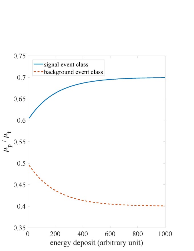 Fig. 1
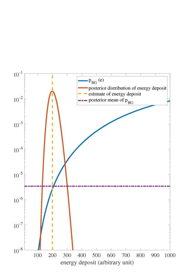 Fig. 2
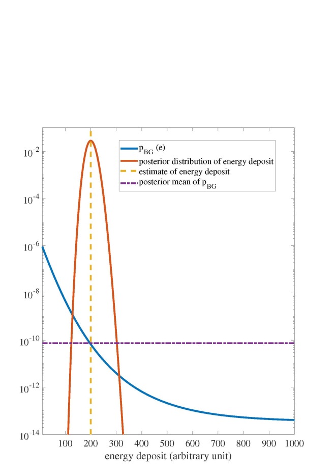 Fig. 3
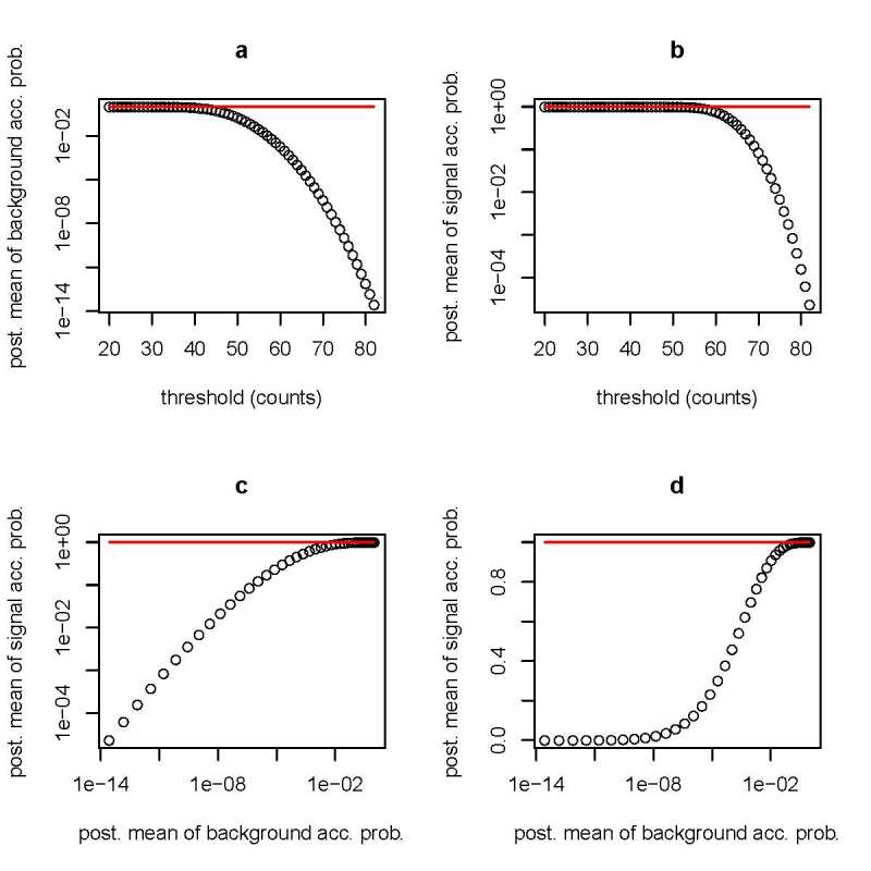 Fig. 4
|
| ||||
| 100 | 6.11 x 10⁻³ | 6.17 x 10⁻³ | 0.508 | 0.512 |
| 200 | 3.31 x 10⁻⁶ | 3.40 x 10⁻⁶ | 0.504 | 0.511 |
| 300 | 2.47 x 10⁻¹⁰ | 2.62 x 10⁻¹⁰ | 0.500 | 0.509 |
|
| ||||
| 100 | 2.34 x 10⁻⁴ | 2.33 x 10⁻⁴ | 0.541 | 0.542 |
| 200 | 7.45 x 10⁻¹¹ | 7.35 x 10⁻¹¹ | 0.512 | 0.513 |
| 300 | 1.27 x 10⁻³⁴ | 9.78 x 10⁻³⁵ | 0.493 | 0.494 |
- —National Institute of Standards and Technology
Peer Reviews
No public reviews on file for this paper yet. If you reviewed it on a platform where reviews are public (OpenReview, ICLR, NeurIPS, ICML), you can paste yours below so the community can read it here.
Videos
No videos yet. Explain this paper in a talk, walkthrough, or lecture? Add one.
Taxonomy
TopicsAnomaly Detection Techniques and Applications · Terahertz technology and applications · Advanced Chemical Sensor Technologies
Introduction
1
In a variety of experiments in fields such as astroparticle physics (for example, see Refs. [1–6]), fast neutron spectroscopy [7–10], and neutrino physics (for example, see Refs. [11–13]), events of interest and background events deposit energy in detectors. Typically, the shapes of measured electronic pulses generated by events of interest and background events are different. There are many different methods [14] for pulse shape discrimination (PSD), including those based on: ratios of pulse integrals corresponding to different time intervals [8, 15, com]parison to reference templates [16–18], machine learning [19–25], pulse gradient methods [26], zero-crossing analysis [27, 28], frequency gradient analysis [29], and Fourier transform analysis [30]. Here, I focus on a “prompt fraction” discrimination statistic F_p_ defined as
where X_p_ is the integrated pulse in a prompt time interval [T_begin_, T_prompt_ ], and X_t_ is the integrated pulse in a total time interval [T_begin_, T_end_ ]. I consider two cases. In one case, X_p_ and X_t_ are correlated Gaussian random variables. In the other case, X_p_ and X_t_ are correlated Poisson random variables.
There are exact and nearly exact approximations for the distribution of the ratio of Gaussian (normal) random variables with known means, variances, and correlation [31–33]. Based on Refs. [31, 32], the work in Ref. [34] includes a model to predict the distribution of prompt fraction statistics produced by a given energy deposit where the observed values of X_p_ and X_t_ are unconstrained. In applications of interest, data generated by a continuum of energy deposits are binned according to observed values of X_t_ . Thus, the conditional distribution of X_p_ given the measured value of X_t_ is of primary interest for PSD studies and the focus of this work.
In many experimental studies, only a fraction of the energy deposited in a detector produces a measurement of interest. In general, this fraction varies for the two event classes. In this work, for each class, I assume that this fraction does not vary from event-to-event. Based on these fractions, I assign a relative yield factor β to each class. For the class with the higher fraction, β = 1. For the other class, 0 < β ≤ 1. If both classes have the same fraction, β = 1 for both classes. Given the full energy deposit e_dep_ and β, I define a scaled energy deposit e as:
For any scaled energy deposit e, I assume that the expected value of X_t_ is the same for both event classes.
For Gaussian and Poisson noise models, I derive exact expressions for the conditional distributions of X_p_ given the measured value of X_t_ and the unobserved value of e. The major technical step to get the analytical result for the Poisson case is well known, but the major technical step to get the analytical result for the Gaussian case is, to the best of my knowledge, a new contribution to the PSD literature. In general, the source that generates events for each class has a potentially broad energy deposit spectrum. For the Poisson case, for each event class, I assume knowledge of the Poisson parameters for a prompt time interval and a late time interval as a function of e. For the Gaussian case, for each event class, I assume knowledge of the mean and variance of the integrated pulse for both a prompt time interval and a late time interval as a function of e. For the cases studied, I assign an event to the signal class if the observed value of X_p_ exceeds a selected discrimination threshold that in general depends on the observed value of X_t_. With a Bayesian method, I determine the posterior mean background acceptance probability as well as the posterior mean signal acceptance probability. My methods should facilitate evaluation of receiver-operating-characteristic curves (signal acceptance probability versus background acceptance probability) [35] for the Gaussian and Poisson cases.
Gaussian Noise Model
2
Conditional Distribution of Xp
2.1
Throughout this work, I denote a random variable with a capital letter (e.g. X) and a particular realization of the random variable with a lower case letter (e.g. x). The prompt fraction statistic is a random variable . I decompose X_t_ into the sum of a prompt and late contribution, i.e.,
where X_p_ is the integrated pulse measured during [T_begin_, T_prompt_ ], and X_l_ is the integrated pulse measured during (T_prompt_, T_end_ ]. Here, I assume that X_p_ and X_l_ are independent Gaussian random variables with known energy-dependent means µ_p_(e) and µ_l_ (e), and known energy-dependent variances and . Given these assumptions, the expected value and variance of X_t_ are
and
Further, the correlation ρ between X_p_ and X_t_ is
As discussed in many references including Ref. [36], if two Gaussian random variables X and Y have correlation ρ, the distribution of the conditional value of Y given the observed value of X, (Y |X = x), is a Gaussian random variable with expected value
and variance
Hence, for the mono-energetic case, given that the observed value of X_t_ is x_t_ and the scaled energy deposit is e, X_p_ is a Gaussian random variable with expected value
and variance
Acceptance Probabilities
2.2
Without loss of generality, I assume that events produced by the signal of interest yield, on average, larger observations of X_p_ (compared to background events) for any particular scaled energy deposit e. Given this assumption, a natural classification rule is to assign an event to the signal class if the observed value of X_p_ exceeds a discrimination threshold c(x_t_) that depends on the observed value of X_t_ . In general, many scientific considerations influence the choice of the discrimination threshold c(x_t_). Given that F(x,µ,σ) is the cumulative distribution function (at x) for a Gaussian random variable with mean µ and standard deviation σ, the background acceptance probability, p_BG_(x_t_,e), is
where µ_p_(x_t_,e,B) is the Eq. (9) prediction of µ_p_(x,e) for the background class, and σ_p_(x_t_,e,B) is the Eq. (10) prediction of σ_p_(x_t_,e) for the background class. The signal acceptance probability is
where µ_p_(x_t_,e,S) and σ_p_(x_t_,e,S) correspond to the Eq. (9) and Eq. (10) predictions for the signal class.
Posterior Means of Acceptance Probabilities
2.2.1
I account for uncertainty in the scaled energy deposit that produces any particular event with a Bayesian method. For a comprehensive review of Bayesian methods, see Ref. [37]. For the ideal case where one has an exact model for the scaled energy deposit spectrum due to background events, the prior distribution for the scaled energy deposit would be equated to this spectrum. However, in general, such an exact model may not be available. For the general case, the prior distribution would be selected by scientific judgement.
I denote the prior distribution for the scaled energy deposit due to a background event as π_BG_(e). For the Gaussian noise model, the conditional probability density function of X_t_ given that E = e is
Without loss of generality, I assume that µ_T_ (e) and σ_T_ (e) are the same for both the signal class and the background class. By Bayes’ theorem, the posterior distribution for E given X_t_ = x_t_ for a background event is
Hence, given x_t_, the posterior mean of the acceptance probability for the background class is
By similar methods, one can derive the posterior mean of the acceptance probability for the signal class as
As a caveat, if the prior distribution for the scaled energy deposit for the signal class differs from π_BG_(e), f_e_(e|x_t_) in Eq. (16) would differ from the corresponding expression in Eq. (15).
Simulation Study
2.3
I assume that energies and integrated voltage pulses are dimensionless. As an illustrative example, I assume that β = 1 [see Eq. (2)] for both classes, and that
and
For the signal class, (α, β) = (0.6,0.1). For the background class, (α, β) = (0.5,-0.1) (see Fig. 1). For both classes,
and
and
The theoretical prompt fraction, µp/µt , varies with the energy deposit for both classes in the simulation experiment. Because the relative yield term β equals 1 for both classes, the scaled energy deposit [see Eq. (2)] and energy deposit agree in this study.
Given the observed value x_t_, I estimate e to be ê = x_t_ . In the primary studies presented here, I set the discrimination threshold c(x_t_) to be the expected value of (X_p_|X_t_ = x_t_, E = ê) for signal events [see Eq. (9)]. This choice corresponds to a target signal acceptance of 0.5. Since µ_t_ (e = x_t_) = x_t_, c(x_t_) = µ_p_(e = x_t_).
In Fig. 2, I illustrate my method for the case where x_t_ = 200 and the prior distribution for e, π_BG_(e), is uniform for the range 10 ≤ e ≤ 1000. At other values of e, the prior distribution is 0. I also determine results for a truncated exponential prior distribution for the range 10 ≤ e ≤ 1000 where
At other values of e, the prior distribution is 0 (see Table 1).
Gaussian noise model where xt = 200 and the discrimination threshold yields a target signal acceptance probability of 0.5. The posterior probability density function distribution of the energy deposit The posterior mean P¯BG derived from Eq. (15), is determined with a uniform prior distribution.
Table 1: Gaussian noise model. Posterior mean of background acceptance probability and posterior mean of signal acceptance probability given that the target signal acceptance probability is 0.5. The exponential prior distribution is defined in Eq. (22).
Predicted Background Spectrum
2.4
In an actual experiment, one might wish to predict the background rate in each of many bins in *x_t_ −space. For an experiment where the expected number of background events is (N_BG_), the predicted number of background events that are assigned to the signal class for values of x_t_ in the interval (x_k_ − ∆/2, x_k_ + ∆/*2) is (N_k_), where
For very narrow bins in x_t_ -space,
Poisson Noise Model
3
I assume that X_p_ and X_l_ are independent Poisson random variables. For the signal class, their Poisson parameters are λ_p_(e,S) and λ_l_ (e,S). For the background class, their Poisson parameters are λ_p_(e,B) and λ_l_ (e,B). Hence, the theoretical prompt ratios for the signal class and background class are
and
Given that N1 and N2 are independent Poisson random variables with Poisson parameters λ1 and λ2 and N = N1 + N2, the conditional distribution of N1, given that the observed value of N is n, is a binomial random variable with parameters n and p where* * This well-known result follows from the following conditional probability equality:
Thus, for the mono-energetic case, given that X_t_ = x_t_, (X_p_|X_t_ = x_t_, E = e) is a binomial random variable with parameters x_t_ and r_S_(e) for the signal class. For the background class, (X_p_|X_t_ = x_t_, E = e) is a binomial random variable with parameters x_t_ and r_BG_(e).
Given that G(k,N,p) is the cumulative distribution function (at k) of a binomial random variable with parameters N and p, the acceptance probabilities for the background and signal classes are
and
By Bayes’ theorem, the posterior distribution for E given X_t_ = x_t_ is
where the conditional probability mass function of X_t_ given that E = e is
where λ_t_ (e) is the expected value of (X_t_ |E = e). Based on Eqs. (28) to (31), the posterior means of the acceptance probabilities for the background class and signal class are then determined with Eq. (15) and Eq. (16).
In a simulation study, I determine posterior mean acceptance probabilities for the Poisson case (see Fig. 3; Table 2). In this study, I set λ_p_(e,S) and λ_l_ (e,S) to the values of µ_p_(e) and µ_l_ (e) assumed for the signal class in Sec. 2.3. I also set λ_p_(e,B) and λ_l_ (e,B) to the values of µ_p_(e) and µ_l_ (e) assumed for the background class in Sec. 2.3. I also set λ_t_ (e) to the value of µ_t_ (e) assumed in Sec. 2.3. I select a threshold corresponding to a target signal acceptance of 0.5. Given x_t_, this threshold is c(x_t_) = x_t_r_S_(e = x_t_).
Poisson noise model where xt = 200 and the discrimination threshold yields a target signal acceptance probability of 0.5. The posterior mean P¯BG derived from Eq. (15), is determined with a uniform prior distribution.
Table 2: Poisson noise model. Posterior mean of background acceptance probability and posterior mean of signal acceptance probability given that the target signal acceptance probability is 0.5. The exponential prior distribution is defined in Eq. (22).
Receiver-Operating-Characteristic Curve
3.1
In Fig. 4, I show how to construct a receiver-operating-characteristic (ROC) curve for any particular value of x_t_ for the Poisson noise model. In this study, x_t_ = 100 and the theoretical model for the Poisson parameters for the prompt and late time intervals for the signal and background are the same as discussed earlier. In Eq. (28) and Eq. (29), the discrimination threshold, c(x_t_), is varied over a broad range of integer values (20 to 83). For each candidate discrimination threshold, I determine the posterior mean value of p_BG_( ,* e*) and the posterior mean value of p_S_( , e) (see Figs. 4a and 4b). Each candidate discrimination threshold yields a distinct value of . The ROC curve is the union of all distinct values of (see Figs. 4c and 4d). One can construct an ROC curve for the Gaussian noise model with a similar approach.
Discussion
4
For both the Poisson and Gaussian models, for any particular energy deposit, I assume that X_p_ and X_l_ are independent random variables (see Sec. 2.1 and Sec. 3). As discussed earlier (see Sec. 1), in many experiments, only a fraction of the full energy deposit produces measurements of interest. As remarked earlier, I assume in this work that this fraction does not vary from event-to-event for each class. If this fraction randomly varies from event-to-event, I expect X_p_ and X_l_ to be positively correlated for any particular energy deposit. The models in this work do not account for this correlation structure.
In the simulations reported here, the posterior mean of the background acceptance probability increases as the energy deposit increases for the Gaussian model (see Fig. 2). In contrast, for the Poisson model, the posterior mean of the background acceptance probability decreases as the energy deposit increases (see Fig. 3). I attribute this result to the fact that the fractional standard deviation (standard deviation divided by expected value) of the conditional value of X_p_ is larger for the Gaussian case relative to the Poisson case.
The choice of prior distribution affected results slightly (see Tables 1 and 2). As a caveat, there may be other prior distributions of interest.
Poisson noise model where xt = 100. (a) Posterior (post.) mean of background acceptance probability (acc. prob.) (P¯BG) versus discrimination threshold. (b) Posterior mean of signal acceptance probability (P¯S) versus discrimination threshold. (c) ROC curve (P¯S versus P¯bg) on log-log scale. (d) ROC curve on log-linear scale. Posterior means are determined with a uniform prior distribution. The horizontal line corresponds to 1.
Summary
5
In this theoretical study, I derived analytical expressions that quantify the performance of a ratio-based pulse shape discrimination method for Gaussian and Poisson noise models. With a Bayesian method, for a particular target acceptance probability for the signal class events, I determined the posterior mean background acceptance probability as a function of the observed value of X_t_ in a way that accounted for imperfect knowledge of the energy deposit. In a simulation study, I determined results for two choices of the prior distribution in the Bayesian method (see Tables 1 and 2).
My analytic methods may enable one to determine receiver-operating-characteristic curves by numerical integration rather than by Monte Carlo simulation. My methods may provide experimentalists with useful theoretical predictions of ratio-based P performance in planning studies provided that integrated pulses are well approximated as realizations of either Gaussian random variables or Poisson random variables, and accurate models for the energy-dependent distributions of X_p_ and X_t_ are available for background events and signal events.
The reference list from the paper itself. Each links out to its DOI / PubMed record.
- 1Borexino Collaboration, Alimonti G, Arpesella C, Back H, Balata M, Beau T, Bellini G, Benziger J, Bonetti S, Brigatti A, Caccianiga B, Cadonati L, Calaprice F, Cecchet G, Chen M, De Bari A, De Haas E, de Kerret H, Donghi O, Deutsch M, Elisei F, Etenko A, von Feilitzsch F, Fernholz R, Ford R, Freudiger B, Garagiola A, Galbiati C, Gatti F, Gazzana S, Giammarchi M, Giugni D, Golubchikov A, Goretti A, Grieb C, Hagner C, Hagner T, Hampel W, Harding E, Hartmann F, von Hentig R, Hess H, Heusser G, Ianni A
- 2Lippincott W, Coakley KJ, Gastler D, Hime A, Kearns E, Mc Kinsey D, Nikkel J, Stonehill L (2008) Scintillation time dependence and pulse shape discrimination in liquid argon. Physical Review C 78(3):035801.
- 3Ueshima K, Abe K, Hiraide K, Hirano S, Kishimoto Y, Kobayashi K, Koshio Y, Liu J, Martens K, Moriyama S, Nakahata M, Nishiie H, Ogawa H, Sekiya H, Shinozaki A, Suzuki Y, Takeda A, Yamashita M, Fujii K, Murayama I, Nakamura S, Otsuka K, Takeuchi Y, Fukuda Y, Nishijima K, Motoki D, Itow Y, Masuda K, Nishitani Y, Uchida H, Tasaka S, Ohsumi H, Kim YD, Kim YH, Lee KB, Lee MK, Lee JS, The XMASS Collaboration (2011) Scintillation-only based pulse shape discrimination for nuclear and electron recoils in
- 4O’Keeffe H, O’Sullivan E, Chen M (2011) Scintillation decay time and pulse shape discrimination in oxygenated and deoxygenated solutions of linear alkylbenzene for the SNO+ experiment. Nuclear Instruments and Methods in Physics Research Section A: Accelerators, Spectrometers, Detectors and Associated Equipment 640(1):119–122.
- 5Amaudruz PA, Batygov M, Beltran B, Bonatt J, Boudjemline K, Boulay MG, Broerman B, Bueno J, Butcher A, Cai B, Caldwell T, Chen M, Chouinard R, Cleveland BT, Cranshaw D, Dering K, Duncan F, Fatemighomi N, Ford R, Gagnon R, Giampa P, Giuliani F, Gold M, Golovko VV, Gorel P, Grace E, Graham K, Grant DR, Hakobyan R, Hallin AL, Hamstra M, Harvey P, Hearns C, Hofgartner J, Jillings CJ, Kuźniak M; Lawson I, La Zia F, Li O, Lidgard JJ, Liimatainen P, Lippincott WH, Mathew R, Mc Donald AB, Mc Elroy T, Mc Fa
- 6Calvo J, Cantini C, Crivelli P, Daniel M, Di Luise S, Gendotti A, Horikawa S, Molina-Bueno L, Montes B, Mu W, Murphy S, Natterer G, Nguyen K, Periale L, Quan Y, Radics B, Regenfus C, Romero L, Rubbia A, Santorelli R, Sergiampietri F, Viant T, Wu (2018) Backgrounds and pulse shape discrimination in the Ar DM liquid argon TPC. Journal of Cosmology and Astroparticle Physics 2018(12):011.
- 7Klein H, Neumann S (2002) Neutron and photon spectrometry with liquid scintillation detectors in mixed felds. Nuclear Instruments and Methods in Physics Research Section A: Accelerators, Spectrometers, Detectors and Associated Equipment 476(1-2):132–142.
- 8Flaska M, Pozzi SA (2007) Identification of shielded neutron sources with the liquid scintillator BC-501A using a digital pulse shape discrimination method. Nuclear Instruments and Methods in Physics Research Section A: Accelerators, Spectrometers, Detectors and Associated Equipment 577(3):654–663.