A Novel High-Fidelity Simulation for Finishing Operations: Hybrid Image Mosaic and Wavelet Decomposition
Yupeng Xin, Wenhui Li, Xun Xu, David Culler

TL;DR
This paper introduces a high-fidelity simulation method combining image mosaic and wavelet decomposition to improve finishing operation accuracy.
Contribution
A novel method combining image mosaic and wavelet decomposition for high-fidelity finishing simulations is proposed.
Findings
The proposed method improves simulation accuracy by over 30%.
The error between the model and actual surface is controlled within 1 μm.
Abstract
In finishing simulations, achieving accurate results can be challenging due to the minimal amount of material removal and the limited measurement range of surface micro-topography instruments. To overcome these limitations, a novel high-fidelity modeling method combining image mosaic and wavelet decomposition technologies is proposed in this paper. We achieve the stitching of narrow field and high pixel micro morphology images through four steps: image feature extraction, overlapped feature matching, feature fusion, and stitching effect evaluation. On this basis, the wavelet decomposition method is employed to separate detection signals based on their respective frequencies, allowing the establishment of a datum plane and a roughness surface. The point cloud model undergoes a transformation into a continuous geometric model via the Poisson reconstruction algorithm. In the case study,…
Genes, proteins, chemicals, diseases, species, mutations and cell lines named across the full text — each resolved to its canonical identifier and authoritative record.
Click any figure to enlarge with its caption.
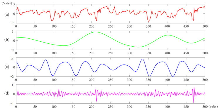 Figure 1
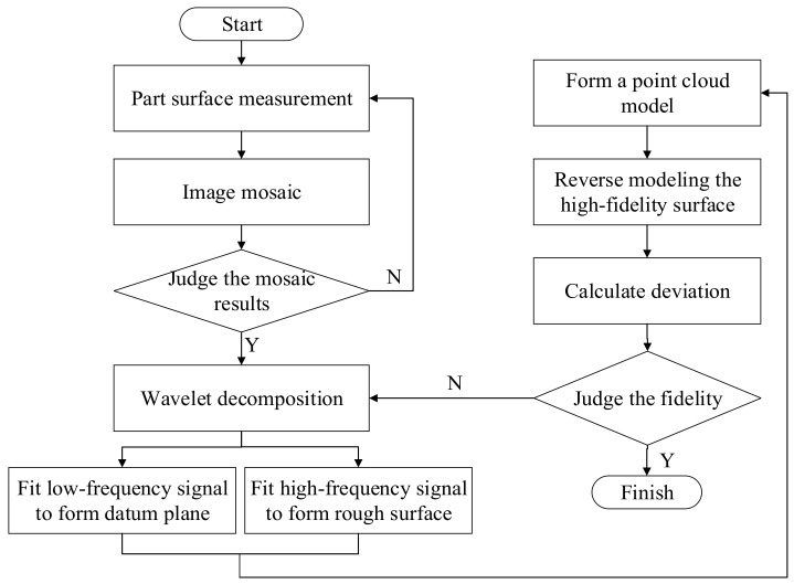 Figure 2
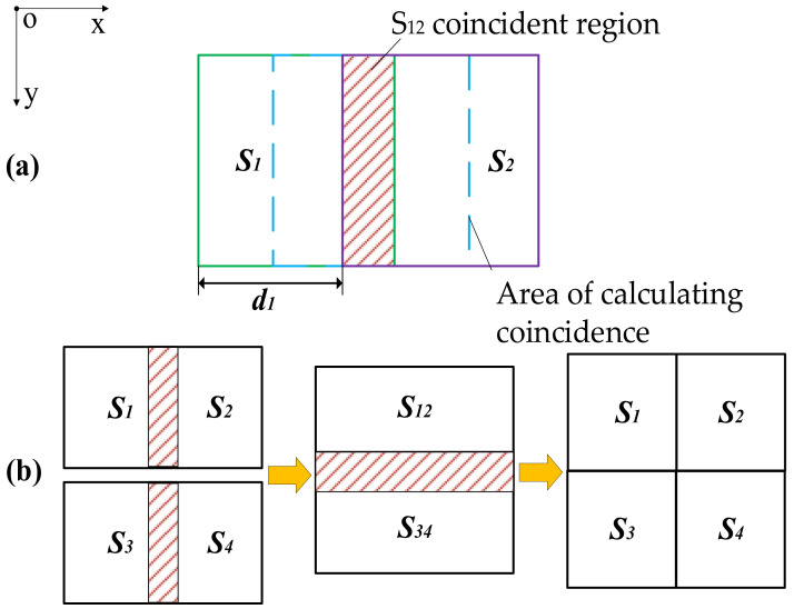 Figure 3
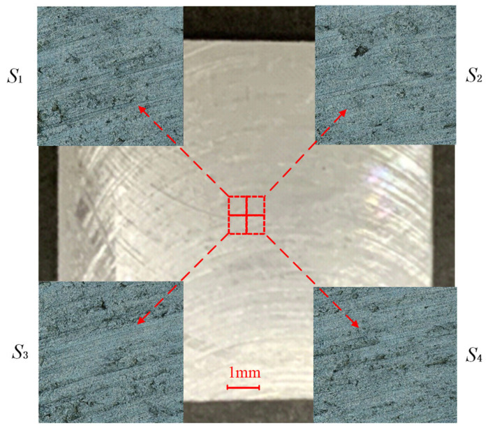 Figure 4
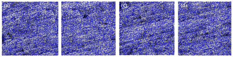 Figure 5
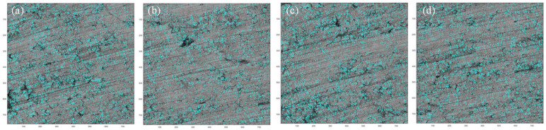 Figure 6
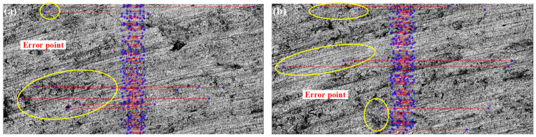 Figure 7
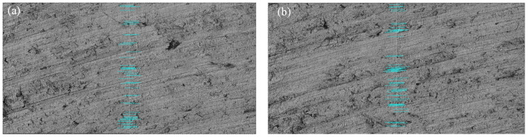 Figure 8
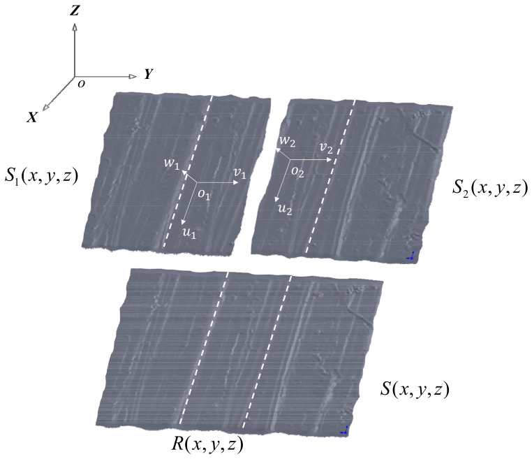 Figure 9
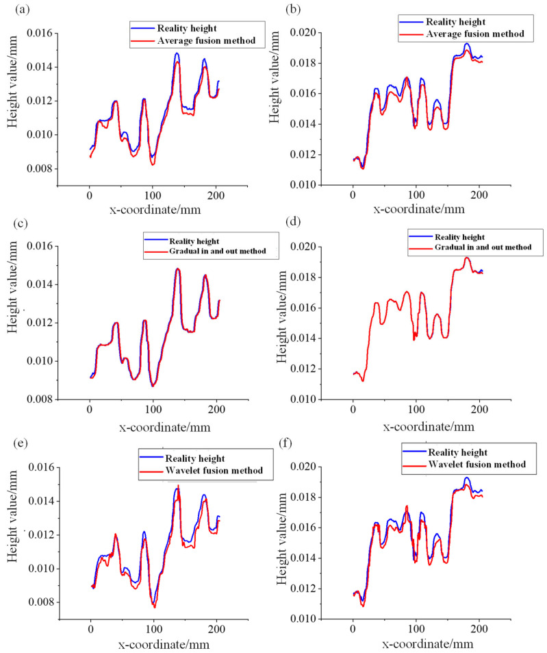 Figure 10
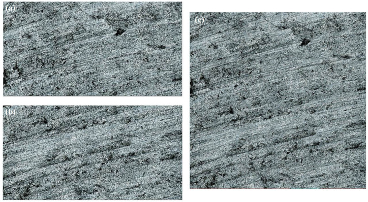 Figure 11
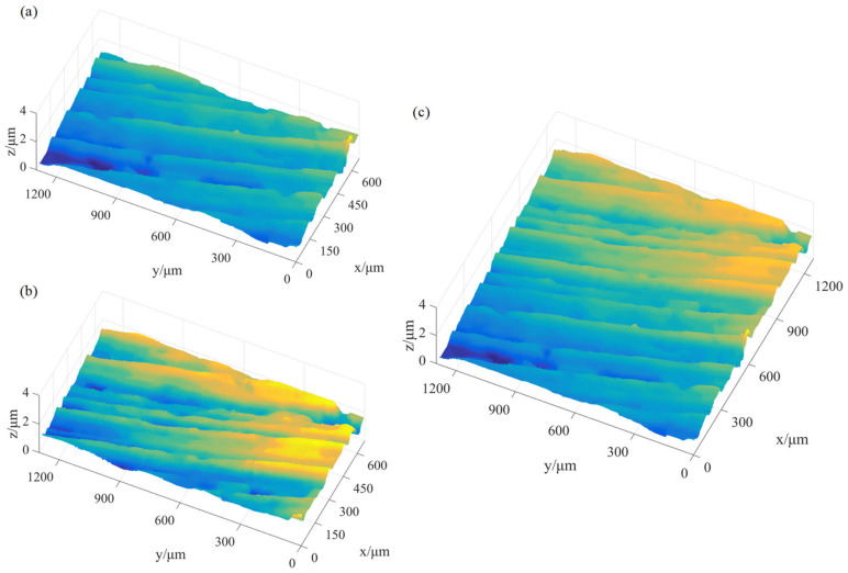 Figure 12
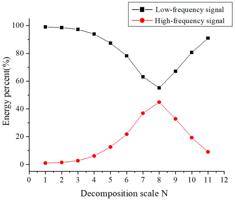 Figure 13
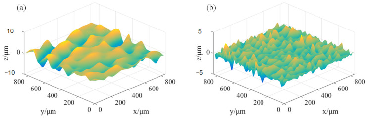 Figure 14
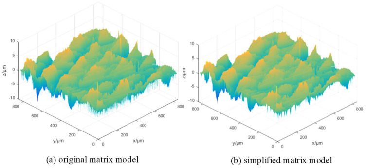 Figure 15
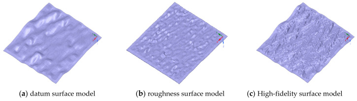 Figure 16
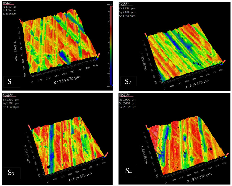 Figure 17
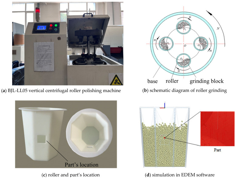 Figure 18
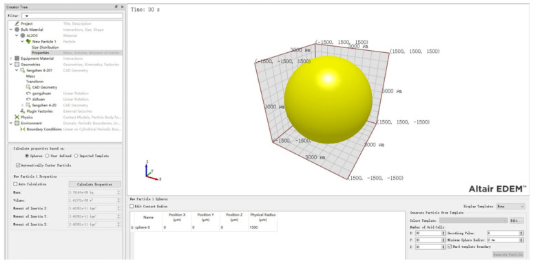 Figure 19
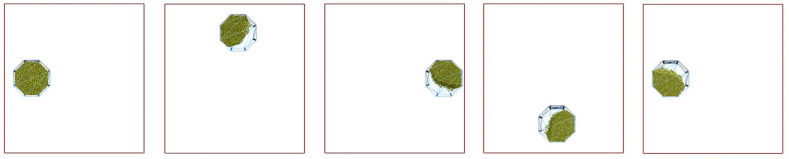 Figure 20
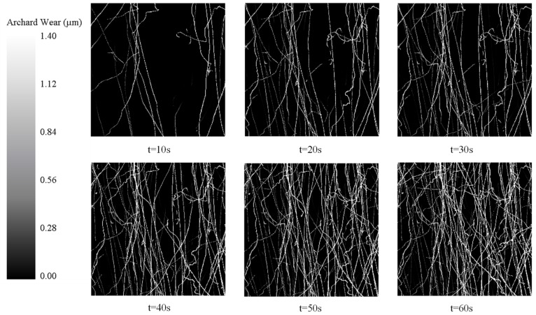 Figure 21
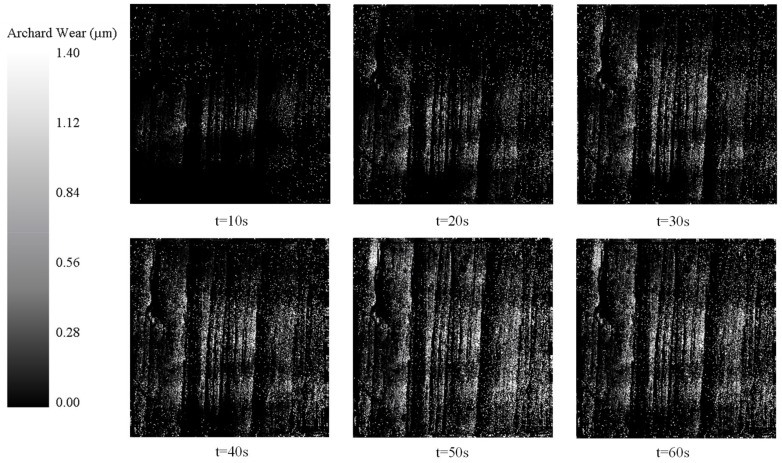 Figure 22
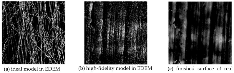 Figure 23
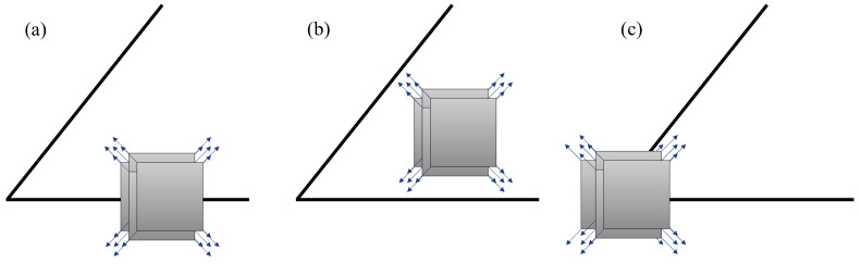 Figure 24
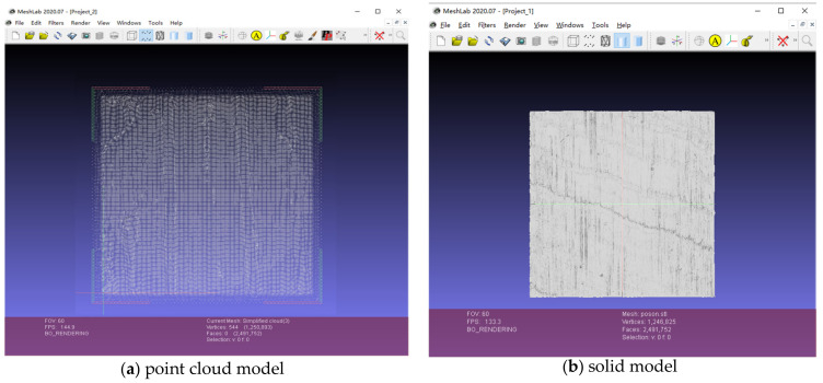 Figure 25
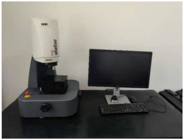 Figure 26
- —National Natural Science Foundation of China
- —China Scholarship Council
Peer Reviews
No public reviews on file for this paper yet. If you reviewed it on a platform where reviews are public (OpenReview, ICLR, NeurIPS, ICML), you can paste yours below so the community can read it here.
Videos
No videos yet. Explain this paper in a talk, walkthrough, or lecture? Add one.
Taxonomy
TopicsOptical measurement and interference techniques · 3D Surveying and Cultural Heritage · Industrial Vision Systems and Defect Detection
1. Introduction
There is a growing trend toward digitalization in manufacturing that allows people to replace machining trials with computer simulation technology. The potential to reduce production costs, eliminate waste, and improve efficiency has attracted the attention of researchers and industry [1]. While early applications of machining simulations focused on optimizing tool paths and predicting tool/holder collisions, the technology has expanded into other areas. With advances in Finite Element Modelling (FEM), there are opportunities for new and innovative metal cutting simulations to be developed [2]. The deformation process of plastic metal chips and the change in cutting surface temperature and pressure can be simulated using FEM. Applying this method, the cutting action is modeled as a Boolean operation, providing moderate simulation times and both relevant and fairly accurate surface topographies [3].
However, the simple Boolean intersection assumption is not directly applicable for the simulation of finishing operations because of the tiny amount of material removed and the lack of a micro-surface topography. In this case, a significant number of examples from the literature represent the finishing process as the cinematic mapping of the tools or particles on the smooth surface [3,4,5,6]. By doing that, the surface shape of the part on the micro scale is ignored. The simulation results based on such an ideal model often differ greatly from reality [7]. Therefore, constructing a high-fidelity surface part model that can be directly applied in the finishing simulation is critical to improve the accuracy and benefits of simulation [6].
The ISO standard 25178 and ASME B46.1 defines a uniform description for surface models using surface texture (surface roughness, waviness, and lay) [8]. An ideal surface model, also known as a Nominal Model, is a continuous surface composed of an infinite number of points on the geometric shape of parts. Subtractive machining processes like milling, turning, and grinding are imperfect by nature, and therefore produce imperfections and deviations in part surfaces such as pits and bumps. A high-fidelity surface model should map these machining defects into the 3D model. There are two distinct strategies for simulating machining deviations on part surfaces.
The CAE-based machining simulation strategy, which simulates the detailed machining process and generates high-fidelity models (known as Schleich) divides geometric deviations into system deviation and random deviation according to GPS standards. Then, it utilizes geometric modeling methods, such as Bezier curves [9,10], Splines [11,12,13], and NURBS [14,15], to establish the system deviation model. The Gaussian process method is used to establish the random deviation model, thereby ensuring that a high-fidelity part surface model is transferred to the CAE system [16,17,18]. The simulation results obtained by this strategy are based on the premise that the ideal processing state remains unchanged and does not include the actual physical state.
To address this deficiency, some researchers study the use of the machine learning method to train high-fidelity models from historical machining data. Jose proposed a reconstruction algorithm that takes as input an incomplete measurement, identifies the statistical shape parameters, and outputs a full scan reconstruction [19]. Nicholas utilized machine learning in the ultra-precision diamond machining of single-crystal germanium to create a model, which demonstrated that by using surface metrology parameters in the model, improvements in fracture prediction can be achieved [20]. Gaikwad used machine learning techniques to train high-fidelity models from historical monitoring data obtained through high-speed imaging, for predicting the size, velocity, and shape characteristics of droplets in the liquid metal jetting additive manufacturing process [21]. The trained high-fidelity models can effectively improve prediction results when processing conditions remain constant.
The second strategy is based on real-time physical detection data. The detected physical signals are converted into numerical values using mathematical statistical methods, and then surface and solid models are generated using geometric modeling techniques. Min uses one-dimensional and three-dimensional random noise to generate the part surface model with shape deviation [22], but because the vertex coordinates of the surface model simulated by random deviation are generated independently, the distance between the two connected vertices may be too large, resulting in a surface that is not smooth. Rui Xiong used a full-dimensional measurement method based on polarized coded aperture correlation holography, which greatly improves the reliability and practicability with respect to conventional measurement methods [23]. Fireman and Xun developed a surface roughness predictive model by obtaining machining parameters, e.g., feed rate, depth of cut, and spindle speed [24].
In recent years, digital twin technology has gained significant traction, promoting an increasing number of scholars to develop digital twin systems that enable the creation of high-fidelity models. Bao proposed a biomimicry-based digital twin modeling method to construct high-fidelity models by fusing machining process data and optimizing the machining process in real-time [25]. Xin proposed a refined simulation method based on digital twin technology, which integrates real-time machining data with a process design system through the integration of CAPP and MES systems. The high-fidelity process model is iteratively generated using real-time inspection data to improve the fidelity of process simulation [26]. Similar methods have also been applied to cutting tools [27,28], machine tools [27,29,30], and process models [31,32,33]. Admittedly, the modeling methods based on the actual detection data are more conducive to improving the overall accuracy of the model.
In practical applications, the accuracy of the aforementioned high-fidelity geometric models is often influenced by various factors such as model complexity, computer performance, and data transmission. In addition, data collected through optical measurement is often affected by environmental interference, equipment errors, and other factors, requiring the filtering and processing of the data [34]. Mean and median filtering are two commonly used basic filtering methods that reduce the influence of outliers by calculating the average and median values of the data, respectively. Liu used median filtering to denoise the vibration signals during the milling of thin-walled workpieces [35]. Si implemented Kalman filtering to estimate the state of the engine support system by establishing a system state model and an observation model [36]. When the signal is extremely unstable, it is usually necessary to adjust the filtering parameters in real-time based on the change or noise characteristics. This type of filtering method is called adaptive filtering. He proposed an adaptive filtering method based on singular values and a mixture of Gaussian models, which accurately identified the tool wear state under different machining parameters [37]. The wavelet transform method is a time–frequency analysis method that decomposes a signal into multiple sub-signals of different frequencies and filters each sub-signal. Its advantage is that it can simultaneously process high-frequency and low-frequency signals. Ahmed used the wavelet transform method to monitor the changes in cutting force signals in stainless steel machining, achieving effective control of the built-up edge [38].
Based on the above research, it is clear that the geometric accuracy of high-fidelity models generated by different filtering methods may vary, making it challenging to ensure consistency. Furthermore, detection signals reflect various geometric morphologies at different scales. Surface roughness and waviness are associated with distinct frequencies and wavelengths, as illustrated in Figure 1. The v/div and s/div refer to the time base unit of the oscilloscope, representing the volt value per grid and seconds per grid, respectively. Therefore, separating, extracting, and processing these signals will significantly affect the accuracy of the surface model.
To address the shortcomings described above, this paper proposes a high-fidelity surface modeling method that combines an image mosaic technology with wavelet decomposition. A flowchart to describe this process is shown in Figure 2.
Following this logic, the paper is structured as follows: Section 2 describes the concept of the image mosaic, Section 3 compares the three different wavelet decomposition methods and describes how the Symlet wavelet was selected to reconstruct the high-fidelity surface model, and Section 4 compares and analyzes the results of the simulation developed and the finishing experiment employed. Finally, conclusions and some areas identified for future research are described.
2. Image Mosaic
The CCD camera imaging system is typically used to image the micro-shape of a surface measured by the 3D topography instrument [39,40]. But, due to the restriction of the lens, the transverse dimension of the measured surface is limited to approximately a 1000 μm × 1000 μm viewing area [32]. When measuring a large area with a high-power lens, it is necessary to expand the field of view of the measured surface. The work presented in this paper employs a method for dividing the surface of the test part into several overlapping sub-areas for the purpose of measuring. The algorithm is designed to cut and splice the overlapping areas and create a larger range of 3D surface topography data.
Using a 2 × 2 image to demonstrate the stitching process, the data acquisition and processing diagram is shown in Figure 3. The splicing steps are as follows: (a) Move the lens to the first detection position to obtain the image S1. (b) Now, move the lens horizontally in the +x direction to the next detection position S2. Here, it is important that the horizontal distance d1 is less than the length of S1 so that images S1 and S2 are overlapped. (c) Next, move the lens back in the −x direction over S12 to obtain the area of calculating coincidence, being sure to completely cover the S12 overlapping area. (d) Repeat the same principle explained above to obtain the overlapping area of S3 and S4. (e) Lastly, complete the splicing of S12 and S34.
To demonstrate the methods proposed in this paper, a 20 mm × 20 mm × 3 mm aluminum alloy sheet is used. The part’s surface is measured with the ZeGage Plus optical profiler, which has sub-nanometer precision and an optical resolution of 0.52 μm. The sampling area selected for use is in the geometric center of the part. By using three equally spaced distances for moving the lens d1, a set of mosaic images with different coincidences are collected. The overlapping areas are about 10%, 20%, and 30% of the original image size. Figure 4 shows the image with a coincidence of 10%. The sampling interval is approximately 0.815 μm. In Figure 4, the image is enlarged by 700% and the result is 1200 × 1200 pixels. The original size of the composite image created using the stitching/splicing process described earlier is 834.37 μm × 834.37 μm.
2.1. Image Feature Extraction
The first step in the image mosaic process is to recognize the features within the overlapping regions. The most widely used feature description methods are the Harris corner algorithm [41] and the Scale-Invariant Feature Transform (SIFT) algorithm [42,43]. An analysis is performed to identify the optimal feature recognition by comparing the results from two algorithms.
(1)Harris corner feature extraction algorithm
A corner is defined as a stable sparse geometric feature in the point cloud data. The Harris algorithm finds corners by sliding the convolution window; when the sliding window moves at various angles, the corner points will be determined when the pixel gray value in the window changes [41]. The details are shown in Appendix A. Figure 5 shows the corner detection results of S1, S2, S3, and S4 in MATLAB 2020, which are 1561, 1551, 1578, and 1582.
(2)SIFT feature extraction algorithm
The SIFT algorithm includes four steps: scale space extreme value detection, key point location, direction assignment, and key point description [44]. The result of stitching an image using the SIFT algorithm in MATLAB is shown in Figure 6. The key point numbers of the four images (S1, S2, S3, and S4) are 1660, 1349, 1670, and 1548.
2.2. Image Feature Matching
After extracting the corresponding corner position of each image, the Normalized Cross Correlation (NCC) is used to match the feature points. Yoo and Han [45] demonstrate the robustness and accuracy of NCC, and its formula is as follows:
where W is the window of feature point. and are the pixel values in the original image. and are the average pixel values in the window.
The matching process consists of the follow steps: First, a point is selected in and its corresponding feature point with the greatest correlation is searched for in . Then, for the selected point in , the feature point with the greatest correlation is searched for in . The matching process is considered to be completed when the feature points with the greatest correlation are found to correspond to each other through a double-way search. The matching efficiency r and Mean Average Precision (MAP) are generally used as two indicators to evaluate the matching effect:
where is the number of correct matching feature points extracted from each image, is the total number of matching feature points extracted from each image, and t is the matching time.
where the accuracy rate is , the recall rate is p.
In the case of three different overlapping areas, the Harris and SIFT algorithms are used to match the two adjacent images, and the results are shown in Table 1. According to Formula (3), the average matching accuracy MAP of the SIFT algorithm and Harris algorithm is 0.539 and 0.474, respectively. As the overlap area increases, the matching time (t) will also increase correspondingly, and the recall rate (R) will gradually increase, resulting in a gradual decrease in the matching efficiency. The matching efficiency of the SIFT algorithm shows more than three times that of Harris algorithm.
Figure 7 (Harris algorithm) and Figure 8 (SIFT algorithm) show the first set of mosaic images in Table 1, respectively. In Figure 7, both of the and have obvious abnormal matching points and sutures. There are no such circumstances in Figure 8.
In Figure 7, we can see that some matching points far from the stitching position have also been identified by the Harris algorithm(as indicated by the yellow circle), which is obviously incorrect. From the comparison of the results above, it can be seen that the SIFT algorithm has higher computational efficiency and reliability in the stitching of three-dimensional micro-surface morphology images. Therefore, this article uses the SIFT algorithm to implement the stitching of the micro-surface morphology images of parts.
2.3. Image Fusion Algorithm
In the image fusion algorithm, and are used to represent point sets for images and . represents the common area of both in the mosaic image , as shown in Figure 9. Since and belong to different coordinate systems, and , in order to obtain the point set S of the mosaic image in the global coordinate system o-xyz, a coordinate geometric transformation is required.
Image fusion can be divided into pixel-level fusion, feature-level fusion, and decision-level fusion. Since the mosaic images discussed in this paper are the images obtained under the same lens, pixel-level fusion is selected. Pixel-level fusion methods usually include the average fusion method, gradual in and gradual out fusion method, wavelet fusion method, etc.
(1)The average fusion method is used to directly add the corresponding height values of the overlapping areas after matching and take the average value. The calculation formula can be expressed as follows:
(2)The gradual in and out method is also known as the linear transition fusion method, and its algorithm can be expressed as follows:
where , is the abscissa value of the left boundary of the overlapping area. is the abscissa value of the right boundary of the overlapping area. is the abscissa of pixel points in the overlapping area. a is a coefficient between 0 and 1. When a changes from 0 to 1, the two images can smoothly transition.
(3)The wavelet fusion method is used to decompose the overlapping regions corresponding to a group of 3D topography images by a two-dimensional discrete wavelet. The morphology image is decomposed into low-frequency coefficients and high-frequency coefficients in three directions. The algorithm can be expressed by the following formula:
where are the decomposition rules for the low-frequency coefficients and high-frequency coefficients, described in detail in the literature [46,47].
Figure 10 shows the fusion results of and using the above three methods, which is to extract the height values of two different interfaces in the overlapping region . It can be concluded that the curve created by the gradual in and out fusion method is the closest to the reality height curve fitting, which represents the actual surface.
2.4. Splicing Effect Judgment
This section evaluates the splicing effect by calculating the structural similarity coefficient SSIM of overlapping areas. Given two images x and y, the SSIM can be expressed as follows:
where and are the average values of x and y. and are the variance of x and y. is the covariance of x and y. L is the dynamic pixel value. and are calculated by formulas and . The and are generally selected to be 0.01 and 0.03 [47]. The value range of SSIM can be found in [47,48]. When taking a value of 1, it means that the two images are identical, while the closer to 1, the better the stitching effect.
Formula (10) can be used to calculate the SSIM value of the overlapping area. Comparing the three fusion algorithms described in Section 2.3, the results are shown in Table 2, which proves that the gradual in and out fusion method is the optimal method.
Therefore, the gradual in and out fusion method is used to splice , . The results are shown in Figure 11 and Figure 12, and its 3D shape size is 1281 1281 .
3. Wavelet Decomposition and Surface Reconstruction
Spliced images created in the previous steps lack the datum features or roughness parameters necessary for simulation and cannot be saved as solid models to import into simulation software for subsequent analysis. Wavelet analysis separates detection signals, digitally establishing datum planes and roughness surfaces. The pooling method from a neural network algorithm simplifies the shape sample data to reduce calculation requirements and build high-fidelity solid models. The results undergo review to ensure accuracy before evaluating error values through a comparison with actual part surface test data.
3.1. Wavelet Decomposition of Detection Signals
The measurement data obtained with the optical profiler are the coordinate values in the X, Y, and Z directions in the measurement area. If the number of samples in the X axis and Y axis are recorded as m and n, respectively, the height matrix of part surface can be expressed as follows:
where is the height matrix of the actual surface topography, is the height matrix of the reference plane composed of low-frequency signals such as surface waviness and geometric shape deviation, and is the height matrix of high-frequency signals composed of surface roughness.
The wavelet transform method is used to decompose the signal at multiple scales. The wavelet base of the wavelet transform method is a curve with a zero value. By stretching and translating it, a family of wavelet functions is obtained. The signal is decomposed into a linear superposition of the family of wavelet functions [4]. The basic idea of 2D wavelet decomposition is to decompose the original signal S into n high-frequency signals (D1, D2, …, Dn) and n low-frequency signals (A1, A2, …, An). Wavelet reconstruction is the inverse process of wavelet decomposition. The reconstructed signal is composed of high-frequency signals at all levels and low-frequency signals at the highest order, which can be expressed as follows:
The selection of wavelet basis function affects the distribution of wavelet coefficients after decomposition, and directly determines the accuracy of the decomposed signal [4,49]. In this paper, based on the principle of minimum reconstruction deviation, different wavelet bases are used to decompose and reconstruct the original signal, and the Root Mean Square Error (RMSE) of is calculated to find the optimal wavelet base.
where is the value of row i and column j in the reconstructed topography height matrix under different wavelet bases, and is the value of row i and column j in the original topography height matrix.
For specific surface data, the decomposition scale l is customized to divide the roughness surface and datum plane:
where is the low-frequency signal coefficient under the decomposition scale l, and is the sum of all high-frequency signal coefficients in the l to l decomposition scale.
Using S1 in Figure 4 as an example to compare the Daubechies wavelet, Symlet wavelet, and Coiflet wavelet, the 3D coordinates of some sampling points of S1 are shown in Table 3. The RMSE results are shown in Table 4 by decomposing and reconstructing the original data with vanishing moments of different orders.
It can be concluded from Table 4 that the optimal wavelet base is sym5, and the minimum reconstruction error is 0.85669 × 10^−19^. Therefore, sym5 is used to decompose the original signal, and the proportion of signal energy at different scales in MATLAB is shown in Figure 13. It can be seen from the figure that the proportion of low-frequency signal energy changes from falling to rising with the increase in decomposition scale N, and the minimum value is obtained when N = 8. Wavelet decomposition conforms to the law of the conservation of energy. The lower the proportion of low-frequency energy, the closer the low-frequency signal is to the reference plane. Therefore, a Symlet wavelet basis is used to decompose S1. Under the condition of order 5 and decomposition level 8, the datum plane and roughness surface obtained are shown in Figure 14.
3.2. Simplification and Reconstruction of Surface Model
In order to improve the computational efficiency, the maximum pooling method in the convolution neural network is used to sample and process the shape data. Pooling has translation invariance, which can reduce the difficulty and number of parameters in the optimization when applied to the neural network [5].
Similarly, it can effectively reduce the amount of data and retain the main features of the original topography when processing the surface topography data. For the height matrix of the reconstructed surface, select the pool filter window size of , step size of a, and the height matrix will be obtained by pool processing. If 1 = m/a, n1 = n/a, the simplified shape height matrix is obtained. The calculation process is as follows: ; ; ; , where is the value of the ith row and the jth column of the surface topography height matrix after down-sampling, and the point cloud model of the datum plane and of the rough surface can be obtained by using the same processing method.
Take S1 in Figure 4 as an example; the reconstructed surface model of S1 can be obtained by overlying the datum and roughness surfaces in Figure 14. The result is shown in Figure 15a, which has the height matrix of 1024 1024. If a = 4 is taken for sampling processing, then the simplified height matrix is 256 × 256, which can be processed in MATLAB, as shown in Figure 15b.
The discrete point cloud model is transformed into a continuous geometric model by the reverse modeling method, which include explicit and implicit reconstruction methods. The explicit method triangulates the point cloud model directly, while the implicit method obtains the final triangulation and extracts the isosurface of the function by reconstructing the implicit function. The Poisson surface reconstruction used in this paper is established by Meshlab, which is detailed in Appendix B. Figure 16c shows the high-fidelity surface model after six times magnification, which is a combination of Figure 16a,b. It can be directly used in the simulation of the machining process.
3.3. Surface Model Deviation Judgement
Deviation detection is an important basis for judging whether the reconstructed surface model is consistent with the actual topography. The surface roughness height parameters , and represent the arithmetic mean height, root mean square height, and maximum height of the three-dimensional surface topography, which depend on the surface height deviation. To verify the precision of the high-fidelity surface model, we compare it with the measured surface and calculate the relative deviation. The calculation process is as follows: ; ; , where, , , and are relative deviations; , , and are calculated based on the actual part surface measurement; are calculated based on the high-fidelity surface model; and e is the threshold.
In this paper, the ZeGage Plus optical profiler is used to obtain the , and of the part, as shown in Table 5. The actual roughness values of the four sample areas are shown in Figure 17.
Table 6 shows the , and values of the four sampling positions ( ) in Figure 4, and compares them with the actual measured values.
Table 6 demonstrates that the maximum relative error obtained at the four sampling positions is 0.909 . In general, the allowable error range for finish machining is within several micrometers. This proves that this method can meet the high-fidelity modeling requirements of finish machined parts within the allowable error range of 1 . Simultaneously, by reconstructing a high-fidelity model after applying wavelet decomposition, the number of grids in the model is significantly reduced, thereby decreasing the computational burden of subsequent machining simulations.
4. Comparison with Experiments
To verify the advantages of the high-fidelity model in the machining simulation, the example in Figure 4 was used for the surface grinding experiment. The discrete element simulation software EDEM2021 is used to simulate the grinding process. The experimental equipment is a BJL-LL05 vertical centrifugal roller polishing machine (shown in Figure 18a). Its working principle is to place the parts, grinding blocks, grinding agents, water, etc., into four evenly distributed cylinders. The cylinder moves in planetary motion. The revolution speed is N, the rotation speed is n, and the speed ratio is n/N. Through the motion created, the grinding block collides, rolls, and micro-grinds the part surface to achieve the finishing of the part surface, as shown in Figure 18b. The roller and installation position of the parts are shown in Figure 18c. Figure 18d is the simulation picture of the grinding experiment in the EDEM simulation.
4.1. Grinding Simulation in EDEM
To simulate roller grinding, four main parameters need to be considered: material parameters, contact parameters, grinding blocks factory parameters, and geometry parameters. The material parameters, as listed in Table 7, comprise the Poisson’s ratio, density, and shear modulus of the rolling grinding blocks, part, and roller.
Contact parameters, displayed in Table 8, encompass the rebound coefficient, static friction coefficient, and rolling friction coefficient between the grinding blocks, part, and roller.
To define the grinding blocks used in the simulation, a spherical block with a diameter of 3 mm, a filling rate of 70%, and a total of 22,000 blocks were specified as the grinding block factory parameters. Figure 19 illustrates the interface of the grinding blocks factory in EDEM2021 software, which includes the blocks mass, volume, and rotational inertia in X, Y, and Z directions.
The revolution speed of the roller is 300 r/min, the revolution radius is 135 mm, and the direction is clockwise. The rotation speed of the drum is 300 r/min and the direction is counterclockwise. The simulation time is 60 s, within which the roller makes planetary motion. The movement track of the roller in one cycle is shown in Figure 20. The time step is set to 20% Rayleigh time, and the calculated time step ∆t = 1.5 × 10^−5^ s.
In the simulation experiment, the wear depth nephogram with a time interval of 10 s is selected to analyze the wear condition of the parts. The wear condition of the ideal surface model and the high-fidelity surface model in the EDEM simulation is shown in Figure 21 and Figure 22. It can be seen from the wear nephogram of the common model that the scratches on the surface of the parts are disorderly. However, the high-fidelity model shows regular wear traces.
4.2. Physical Experiment Results
After 5 min of machining, the surface roughness of changes from 1.272 μm reduced to 0.565 μm. The of is reduced from 1.624 μm to 0.708 μm. The of is reduced from 15.262 μm to 6.162 μm. Figure 23 is used to compare the wear nephogram of the ideal model and the high-fidelity model in the EDEM simulation with the image of the parts after actual grinding.
In light of the excessive computational complexity, the experimental results were solely compared after 60 s of simulation processing. The similarity between Figure 23a,c denoted as SIM1 and SIM2, represents the similarity between Figure 23b,c. The similarity value is obtained by calculating the normalized correlation coefficient of the two images [22], as shown in Formula (12).
where A_mn_ and B_mn_ are the value of the mth row and nth column in the gray value matrix A and B of the two images. and are the average of the pixels of the matrix.
Using Formula (12), SIM1 = −0.0237 and SIM2 = 0.3093 are obtained. The experimental comparison proved that this method is an improvement on current simulation accuracy by more than 30%. That is, compared with the ideal model, the high-fidelity model is more in line with the wear situation in the actual part surface.
5. Conclusions and Future Work
This paper proposed a novel method for developing a high-fidelity surface model. The experiments show that the simulation accuracy can be improved by more than 30% using the high-fidelity model compared with the ideal model. The method of the image mosaic can effectively compensate for the shortcomings of the measuring lens. It makes it possible to obtain a wide range of high-precision part surface panoramas. Some deficiencies of the paper still need further study. It can be seen from the comparison of simulation results in Figure 23 that although the result of SIM2 is much higher than that of SIM1, it also took 96.708 h to complete this simulation, which was undertaken by a computer with an Intel i7-10700 processor (Intel corporation, Santa Clara, CA, USA), a main frequency of 2.9 GHz, a 32 GB memory, and a 16-core CPU.
In the field of high-end manufacturing, high-precision CNC machining machines have demonstrated remarkable accuracy, often achieving tolerances as low as 0.001 mm. Industries such as MEMS (Micro-Electro-Mechanical Systems) and optical component manufacturing demand even greater levels of precision, necessitating a surface machining accuracy at the micron or sub-micron level. Consequently, the development of high-fidelity models is crucial to meet these requirements. However, when analyzing the data collected from optical measurements, discrepancies arise due to variations in the results obtained through different filtering methods. Surprisingly, the existing literature rarely addresses the effectiveness of utilizing these high-fidelity models in machining simulations. This article aims to address this gap by providing valuable insights and supplementary experiments on this important topic. In future work, we will try to use different mathematical statistical methods to simplify the sampling of the data, and in this way, reduce the calculations. Moreover, with the improvement of computer computing capacity, the method proposed in this paper is expected to be more easily applied in practical applications.
The reference list from the paper itself. Each links out to its DOI / PubMed record.
- 1Yip W.S. To S. Zhou H. Current status, challenges and opportunities of sustainable ultra-precision manufacturing J. Intell. Manuf.2022332193220510.1007/s 10845-021-01782-3 · doi ↗
- 2Lotfi M. Akbari J. Finite element simulation of ultrasonic-assisted machining: A review Int. J. Adv. Manuf. Technol.20211162777279610.1007/s 00170-021-07205-0 · doi ↗
- 3Euzenat C. Lavernhe S. Tournier C. Simulation of finishing operations based on an implicit representation of surfaces CIRP J. Manuf. Sci. Technol.202031789010.1016/j.cirpj.2020.09.005 · doi ↗
- 4Li W. Zhang L. Li X. Yang S. Wu F. Theoretical and simulation analysis of abrasive particles in centrifugal barrel finishing: Kinematics mechanism and distribution characteristics Powder Technol.201731851852710.1016/j.powtec.2017.06.033 · doi ↗
- 5Wang X. Yang S. Li W. Wang Y. Vibratory finishing co-simulation based on ADAMS-EDEM with experimental validation Int. J. Adv. Manuf. Technol.2018961175118510.1007/s 00170-018-1639-0 · doi ↗
- 6Zhao Z. Wang S. Wang Z. Wang S. Ma C. Yang B. Surface roughness stabilization method based on digital twin-driven machining parameters self-adaption adjustment: A case study in five-axis machining J. Intell. Manuf.20223394395210.1007/s 10845-020-01698-4 · doi ↗
- 7Kadir A.A. Xu X. Towards High-Fidelity Machining Simulation J. Manuf. Syst.20113017518610.1016/j.jmsy.2011.04.004 · doi ↗
- 8ISO 25178-603Geometrical Product Specifications(GPS)—Surface texture 1st ed.ISO Geneva, Switzerland 2013