Woody plant species richness and productivity relationship in a subtropical forest: The predominant role of common species
Yudan Sun, Silin Chen, Haofeng Ouyang, Shuang Liu

TL;DR
This study shows that in subtropical forests, a few common woody plant species largely drive productivity, not the total number of species.
Contribution
The study demonstrates that common species, not total species richness, predominantly influence productivity in subtropical forests.
Findings
Species richness positively correlates with aboveground biomass.
Common species dominate in abundance and dominance despite being a small fraction of total species.
Common species richness better predicts productivity than total species richness.
Abstract
A long-standing key issue for examining the relationships between biodiversity and ecosystem functioning (BEF), such as forest productivity, is whether ecosystem functions are influenced by the total number of species or the properties of a few key species. Compared with controlled ecosystem experiments, the BEF relationships in secondary forest remain unclear, as do the effects of common species richness and rare species richness on the variation in ecosystem functions. To address this issue, we conducted field surveys at five sampling sites (1 ha each) with subtropical secondary evergreen broad-leaved forest vegetation. We found (1) a positive correlation between species richness and standing aboveground biomass (AGB); (2) that common species were primarily responsible for the distribution patterns of species abundance and dominance; although they accounted for approximately 25% of…
Genes, proteins, chemicals, diseases, species, mutations and cell lines named across the full text — each resolved to its canonical identifier and authoritative record.
Click any figure to enlarge with its caption.
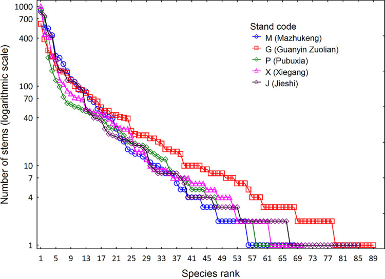 Fig 1
Fig 1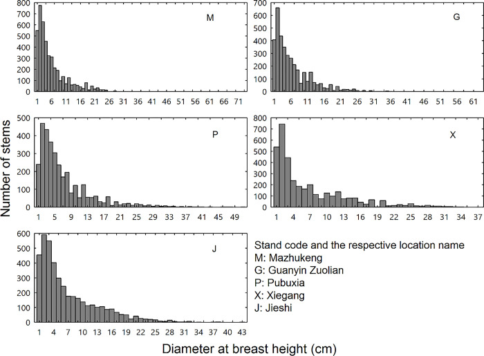 Fig 2
Fig 2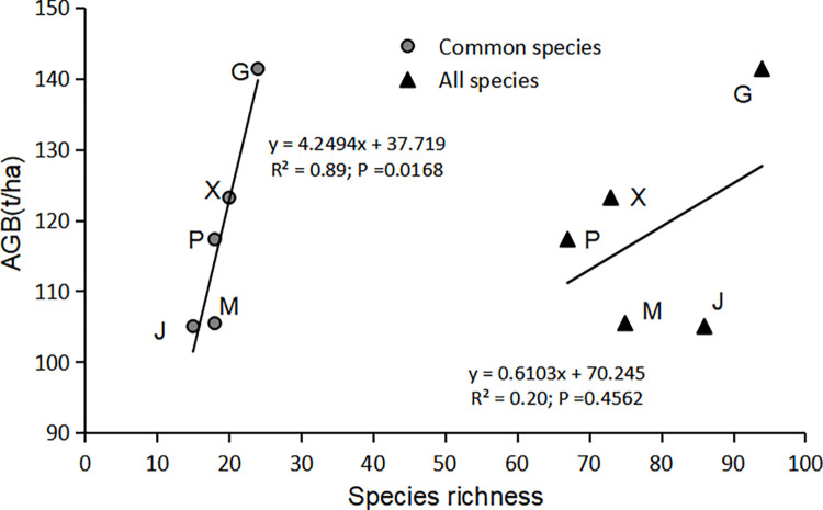 Fig 3
Fig 3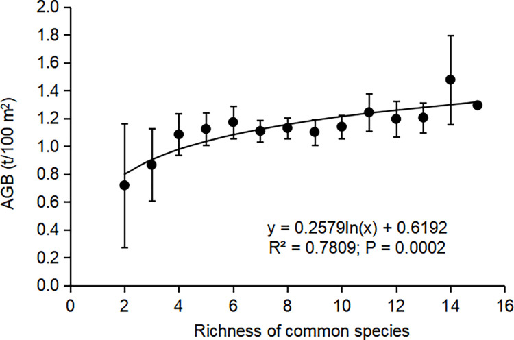 Fig 4
Fig 4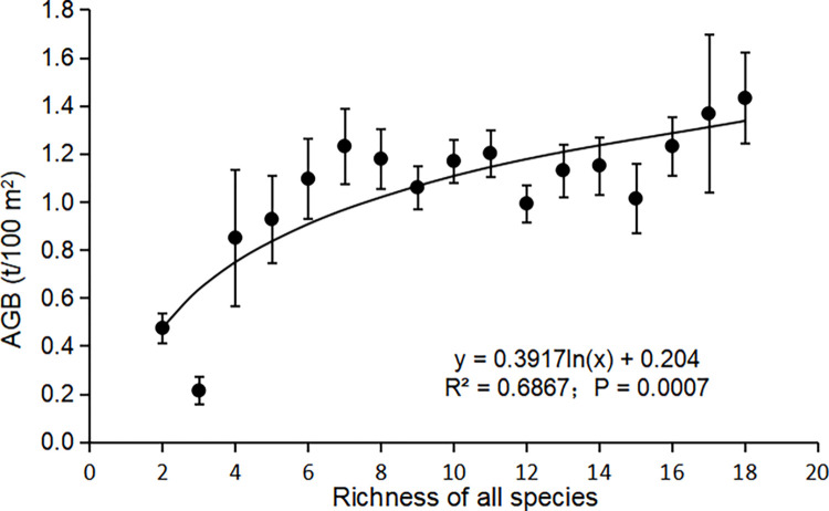 Fig 5
Fig 5- —Science and Technology Bureau of Zhanjiang
- —http://dx.doi.org/10.13039/501100014907Lingnan Normal University
Peer Reviews
No public reviews on file for this paper yet. If you reviewed it on a platform where reviews are public (OpenReview, ICLR, NeurIPS, ICML), you can paste yours below so the community can read it here.
Videos
No videos yet. Explain this paper in a talk, walkthrough, or lecture? Add one.
Taxonomy
TopicsEcology and Vegetation Dynamics Studies · Forest Management and Policy · Conservation, Biodiversity, and Resource Management
Introduction
During the past 20 years, an increasing number of studies have investigated how biodiversity influences ecosystem functions and, in turn, affects human society [1–5]. However, to date, no consistent conclusions regarding the nature, shape, and explanatory power of the relationships between biodiversity and ecosystem functioning (BEF) have been reached [6, 7]. The sampling effect theory suggests that some dominant species in communities will affect the BEF relationship [8, 9], while other studies have suggested that the total number of species is much more important than the properties of a few key species [10]. The productivity-diversity theory states that an increase in biomass will lead to the competitive exclusion of subdominant species and a reduction in biodiversity [11]. The biodiversity-ecosystem functioning theory suggests that an increase in species richness will lead to an increase in biomass due to niche complementarity and positive interspecific interactions [12, 13]. However, a recent study suggested that the community assembly affects BEF relationships, although the random sampling effect did not explain those relationships well [6]. Different response patterns of BEF relationships, such as linear, U-shaped, and unimodal, have been described in previous studies [6, 10, 14–17]. Although these theories and discussions have not resulted in definite conclusions, they have increased the awareness of BEF relationships. However, most of these experiments were conducted in small-scale or controlled environments, and such uniform community experiments with perfect constructions and simulations may overestimate the BEF relationship. Secondary forest may yield different results that might be more representative and better reflect the environmental factors affecting plant communities [18, 19].
The composition of the community structure and proportions of species in secondary forest differ from those in controlled environments, therefore the results of BEF relationships differ from natural and controlled experiments. Aboveground biomass (AGB) depends substantially on the dominant or super-dominant species, which are the most abundant and occupy the highest level in the dominance hierarchy [6, 20, 21]. Because rare species are sensitive to changing environmental conditions, they cannot exist for very long in communities, and the suitable habitats for rare species are always rare [22, 23]. Therefore, species richness-productivity patterns are usually driven by the common species. In studies of BEF in secondary forest rare species may be less predictable than common species [23, 24]. Thus, if we do not differentiate the effects of common species from those of rare species, then redundant variance may be introduced when explaining species diversity-productivity relationships; further, any extraneous or confounding information will interfere with the accuracy of the results.
In view of these issues, we selected five sites (1 ha each) in subtropical forests to explore the relationship between species diversity and productivity in larger-scale secondary forest compared to controlled experiments and aimed to differentiate the explanatory effects of common species from those of rare species on biomass variation(The species studied in this paper include only trees, shrubs and woody vines). According to the niche complementarity theory, the existence of different species increases the efficiency of resource utilization, especially in subtropical forests with distinct layers. Therefore, we propose the following hypotheses: (1) There is a significant positive correlation between species richness and aboveground biomass. Additionally, unlike in controlled experiments, the species distribution is uneven and the density of each species is neither the same nor in a fixed proportion in secondary forest; for this reason, the effect of each species on ecosystem functioning is not equivalent. (2) Thus, the richness of common species explains more of the variation in AGB than the richness of all species. In this study, we analyzed the correlation between species richness with aboveground biomass in the subtropical forests, and further explored the role of common species in natural ecosystems on community productivity. This paper also reveals the interpretation and prediction of the relationship between species richness and productivity by a few common species in subtropical forest ecosystems. We proved that AGB is closely related to common species, which provides a new idea for forest management and conservation: future biomass surveys will only measuring the common species, saving a lot of time and cost.
Materials and methods
Study area
This study was conducted in the Yinping Mountain Nature Reserve of Guangdong Province (114°14′ E, 22°54′ N). The nature reserve covers an area of 2518.3 ha. The mean annual temperature in this area is 21–22°C. The average minimum temperature of the year is 13–14°C in January, while the average maximum annual temperature is 27–28°C in July. The annual rainfall is 1767.8 mm and occurs primarily from April to September, and the average relative humidity is 79% [25, 26]. In the nature reserve, lateritic red soil occurs below an altitude of 600 m, whereas yellow soil is present at higher elevations [25, 26]. The nature reserve belongs to subtropical monsoon climate, and its vegetation types are diverse, including evergreen broad-leaved forest, lowland evergreen monsoon forest and other types. There are abundant animal and plant resources in the reserve. At present, more than 1500 kinds of wild vascular plants and 170 kinds of terrestrial vertebrates have been found [25, 26]. The forest origins of the five stands in the study area were the artificial forest. In 1999, the harvesting of trees was stopped. In order to promote the forest regeneration, artificial tree species such as Schima superba Gardn. et Champ., Acacia magium Wild. and Albizia falcata (L.) Baker et Merr. were replanted. After planting, close hillsides to facilitate afforestation without human interference, and succession was carried out in a completely natural environment.
Experimental design and sampling
In 2020, we designated five forest stands at five sites (1 ha each) located more than 2 km from one another in the Yinping Mountain Nature Reserve of Guangdong Province. The sites were coded as M, G, P, X, and J using the initials of their location names, i.e., Mazhukeng, Guangyin Zuolian, Pubuxia, Xiegang, and Jieshi (Table 1). We set up plots on each site using the contiguous grid quadrat method and conducted a survey of trees in each 10×10-m plot. The woody plants we investigated included trees, shrubs and woody vines. We recorded woody plants with a diameter at breast height (DBH) ≥ 1 cm, and measured the DBH, height, and density of all individuals in each plot.
Table 1: Plant community and habitat overview.
Species abundance classification
For each species (DBH ≥ 1 cm), we calculated the relative abundance (RA), relative frequency (RF), relative dominance (RD), and importance value (IV, IV = RA+ RF+RD) based on the abundance, frequency, and tree basal area. We classified each species as rare or common based on the average relative abundance of <1% (rare) or ≥1% (common) at each site [27, 28].
Stand volume
We calculated the stand volume using bivariate volume equations provided by the Guangdong Institute of Forest Inventory and Planning [29], as follows:
The bivariate standing tree volume equation for Pinus massoniana:
The bivariate standing tree volume equation for Cunninghamia lanceolata:
The bivariate standing tree volume equation for Castanopsis fissa:
The bivariate volume equations for hardwood species in general:
Where V is individual volume (m^3^), D is the trunk diameter (cm) measured 1.3 m above the ground, and H is the height of the tree (m). The sum of the individual volumes from each site or each plot was used to obtain the stand volume at the site or plot level.
Biomass calculation
We used the continuous function method of the biomass expansion factor [30] to calculate the AGB: Where Y is the biomass of the forest stand (t·ha^-1^), X is the stand volume density (m^3^·ha^-1^), and a and b are constants. The parameters, hence, the a and b constants, from studies in areas with similar climates were preferably used in the regression equations to calculate the biomass from the volume. The biomass of bamboo was calculated as 22.5 kg·plant^-1^ [31], while the biomass of other forest types was calculated as follows:
The equation for evergreen broad-leaved forest (Gand J Community) in general [32]:
The equation for Acacia confusa mixed broad-leaved forest (X Community) [33]:
The equation for hardwood forest (Mand P Community) [30]:
Data analysis
We calculated species richness, relative abundance (RA), relative frequency (RF), relative dominance (RD), and importance value (IV). Species richness is the number of species at the site or plot level, while importance value is the sum of three species-specific relative values, RA, RF, and RD.
Kruskal-Wallis test for significant difference were used to analyze the variations in species richness for both common species and rare species across sites. We used regression analysis to evaluate the relationship between AGB (the response variable) and common and total species richness (the predictor variables) at both the site and plot scales. All analyses were performed with the software STATISTICA 8.0 (Statsoft. Inc., Tulsa, OK, USA).
Results
Species richness and abundance
The rank-abundance curves of the five forest stands followed a log series distribution [34], but the richness, total abundance and abundance of the most dominant species varied (Fig 1). The total number of species for the stands M, G, P, X, and J was 68, 89, 66, 70, and 85; the total abundance for each stand was 4375, 3683, 3289, 3668, and 4177; and number of stems of the most abundant species for each stand is 901, 609, 918, 1012, and 841, respectively (Fig 1). The common species with relative abundances ≥ 1%, by definition, had high plot occurrence, whereas the rare species with lower abundances had low plot frequency. Consequently, the plot average for rare species richness was remarkably lower than for common species richness, although the total rare species richness was markedly greater than the total common species richness at the site scale (Table 2).
Rank-abundance curves of the five forest stands, showing abundance and dominance patterns.
Table 2: The richness of common species and rare species for each stand and their contributions to relative abundance (RA) and relative dominance (RD) at five sites.
Community structure
The patterns of tree size distribution varied across the five forest stands (Fig 2). The species with the largest tree DBH for the forest stands M, G, P, X and J were Schima superba (73 cm DBH), Sterculia lanceolata (63 cm DBH), Castanopsis fissa (51 cm DBH), Castanopsis fissa (37 cm DBH) and Machilus chinensis (37 cm DBH), respectively. For all forest stands, most tree stems were small-sized (Fig 2), while in subtropical forests, the small proportion of large trees contributes heavily to the aboveground biomass [35]. The number of trees with a DBH ≥ 5 cm for the forest stands M, G, P, X and J was 1966, 1832, 1782, 1705, and 2179, respectively (Fig 2).
Histograms showing the distribution of diameter at breast height in the five forest stands.
The most abundant and frequent species differed across the five stands based on the abundance and frequency ranks. However, when ranked by the overall estimate of importance, Schima superba had the highest value and thus is the most dominant species in the stands M, G, P, and J, while the dominant species for stand X was Acacia mangium (Table 3). Subdominant species varied across the five stands (Table 3). By representing a small proportion of the total species richness, these dominant and subdominant species accounted for a large proportion of the importance value (Table 3). Similarly, the small proportion of common species (approximately 25% of the total species in each stand) was responsible for the overwhelming proportion of abundance and dominance (Table 2).
Table 3: Structural parameters of dominant species in each of the five stands.
Relationship between species richness and AGB
The number of common species in all the stands was much smaller than the number of rare species. The ratio of common species to rare species was approximately 1:3 at the stand level. However, not only was the frequency of occurrence of common species much greater than that of rare species, but the common species also contributed the most to the abundance (the range of RA was 86.37–91.28) and relative dominance (the range of RD was 88.28–97.34) (Table 2). Based on these results, the common species determined the community structure and thus determined the AGB.
The Shapiro-Wilk test has been performed on common species richness, total species richness and aboveground biomass in each stand, and the three variables all obey the normal distribution (Table 4). At the site scale, although the correlation between total species richness and AGB was not significant (Fig 3; R^2^ = 0.20, P = 0.4562), there was a significant positive correlation between the common species richness and AGB (Fig 3; R^2^ = 0.89, P = 0.0168). At the plot scale, regression analysis revealed that the common species richness could better explain the variation in AGB (Fig 4; R^2^ = 0.78, P = 0.0002) compared to the total species richness (Fig 5; R^2^ = 0.69, P = 0.0007). Thus, eliminating the effect of rare species yielded more significant positive correlation in our study of the relationship between species richness and AGB in the subtropical forest ecosystems.
Relationship between species richness and AGB at the site scale.Abbreviation: AGB, Aboveground biomass; M, G, P, X, and J respectively represent Mazhukeng, Guangyin Zuolian, Pubuxia, Xiegang, and Jieshi.
Relationship between the common species richness and AGB at the plot scale.Plotted values are means ± standard error. Abbreviation: AGB = Aboveground biomass.
Relationship between the richness of all species and AGB at plot scale.Plotted values are means ± standard error. Abbreviation: AGB = Aboveground biomass.
Table 4: Shapiro-Wilk test of common species, total species and aboveground biomass in each.stand.
Conclusions and discussion
Relationships between species richness and productivity
The relationships between species richness and productivity show differently in different plant community types and under different environmental conditions. An earlier study reported a statistical analysis of approximately 200 experimental results for the BEF relationships and found that 30% were unimodal curves, 26% were positive linear relationships, and 12% were negative linear relationships, whereas the last 32% showed no obvious relationships [36]. However, in the grassland ecosystem, the experimental data tended to support the hypothesis that species richness and productivity are positively correlated [10, 37]; thus, increasing niche separation would lead to complementation or promotion within species. Species diversity also promoted nutrient cycling within the ecosystem, and the high-yield species had a greater probability of survival [38–40]. These mechanisms and theories could be treated as an explanation for the hypothesis that species richness and productivity are positively correlated. This hypothesis was also supported by the results of our study. In our study, species richness was positively correlated with ecosystem productivity at both the site and plot scales, which is consistent with our first hypothesis. This might be due to the environmental conditions in the subtropical areas with ample precipitation and sunshine, in which this study was conducted. Some researchers have suggested that highly productive habitats develop more easily in tropical areas with high temperatures and precipitation [41]. Therefore, the tropical and subtropical areas should have larger species pools and higher productivity and will likely fit better with the positive linear model [11]; whereas the unimodal model is more likely to be well suited to temperate regions.
The role of common species and rare species in explaining BEF relationships
The results of field experiments differ from those of controlled experiments, as it is not possible to precisely control environmental conditions nor to generate a uniform species composition and distribution in the former [42, 43]. The impact of rare species on ecosystem functions has been included in the biodiversity-ecosystem productivity model used in controlled experiments. In field experiments, when rare species and common species are considered equivalent, this leads to redundant information in the biodiversity-ecosystem productivity model that reduces its accuracy and, as a result, we cannot fully understand the BEF relationships. Moreover, compared with strictly controlled experiments, experiments in secondary forest are limited by unstable environmental conditions, the initial species composition, and limited resources, all of which strongly vary [39, 44]. Furthermore, a sufficiently long succession time could drive competition between species and lead to the coexistence of species groups with different resource utilization efficiencies and varying performance during the long-term natural succession. Our results showed that common species, which accounted for approximately 25% of the species pool in the sample plot, contributed to 86.37–91.28% of total plant abundance and 86.37–97.34% of woody plant basal area, which is referred to as woody plant dominance. Clearly, common species determined the distribution patterns of community abundance and dominance, which directly affected the community structure and properties. At the site scale, the richness of all species was not able to explain the variation in biomass, whereas the common species richness was able to explain 89% of the variations in biomass. At the plot scale, common species richness better explained and predicted the variation in biomass than did total species richness. Therefore, in the biodiversity-ecosystem productivity model for a secondary forest, the rare species richness was in one way redundant because its effect was not equivalent to that of common species richness when explaining variation in productivity. When the influence of rare species is included, the biodiversity-ecosystem productivity model contains redundant information. These results are consistent with our second hypothesis. From this perspective, it is possible that the BEF relationship is more likely to be determined by a few key species.
Supporting information
S1 Data(XLS)
The reference list from the paper itself. Each links out to its DOI / PubMed record.
- 1Yasuhara M, Doi H, Wei CL, Danovaro R, Myhr SE. Biodiversity-ecosystem functioning relationships in long-term time series and palaeoecological records: deep sea as a test bed. Philos. T. R. Soc. B. 2016;371(1694): 20150282. doi: 10.1098/rstb.2015.0282 27114583 PMC 4843702 · doi ↗ · pubmed ↗
- 2Clark CMD Tilman. Loss of plant species after chronic low-level nitrogen deposition to prairie grasslands. Nature. 2008;451(7179): 712–715.18256670 10.1038/nature 06503 · doi ↗ · pubmed ↗
- 3Lecerf A, Richardson J S. Biodiversity-ecosystem function research: Insights gained from streams. River Res. Appl. 2010;26(1): 45–54.
- 4Kominoski JS, Hoellein TJ, Leroy CJ, Pringle CM, Swan CM. Beyond species richness: Expanding biodiversity-ecosystem functioning theory in detritus-based streams. River Res. Appl. 2010;26(1): 67–75.
- 5Pinho P, Casanelles-Abella J, Luz AC, Kubicka AM, Branquinho C, Laanisto L, et al. Research agenda on biodiversity and ecosystem functions and services in European cities. Basic and applied ecology. 2021;53: 124–133.
- 6Jaillard B, Rapaport A, Harmand J, Brauman A, Nunan N. Community assembly effects shape the biodiversity-ecosystem functioning relationships. Funct. Ecol. 2014; 28(6): 1523–1533.
- 7Wright AJ, Barry KE, Lortie CJ, Callaway RM. Biodiversity and ecosystem functioning: Have our experiments and indices been underestimating the role of facilitation? Journal of Ecology. 2021; 109(5): 1962–1968.
- 8Huston MA. Hidden treatments in ecological experiments: re-evaluating the ecosystem function of biodiversity. Oecologia. 1997;110(4): 449–460. doi: 10.1007/s 004420050180 28307235 · doi ↗ · pubmed ↗