The devil is in the detail: Environmental variables frequently used for habitat suitability modeling lack information for forest‐dwelling bats in Germany
Lisa Bald, Jannis Gottwald, Jessica Hillen, Frank Adorf, Dirk Zeuss

TL;DR
This study shows that using detailed environmental data improves habitat models for forest-dwelling bats in Germany, highlighting the need for more precise data in conservation planning.
Contribution
The study demonstrates that targeted land cover and LiDAR data improve habitat suitability models for forest bat species.
Findings
Incorporating tree species composition and LiDAR data improved model performance for three bat species.
Distribution maps varied significantly based on the level of detail in environmental variables.
Coarse environmental variables may inadequately represent habitat needs of specialized species.
Abstract
In response to the pressing challenges of the ongoing biodiversity crisis, the protection of endangered species and their habitats, as well as the monitoring of invasive species are crucial. Habitat suitability modeling (HSM) is often treated as the silver bullet to address these challenges, commonly relying on generic variables sourced from widely available datasets. However, for species with high habitat requirements, or for modeling the suitability of habitats within the geographic range of a species, variables at a coarse level of detail may fall short. Consequently, there is potential value in considering the incorporation of more targeted data, which may extend beyond readily available land cover and climate datasets. In this study, we investigate the impact of incorporating targeted land cover variables (specifically tree species composition) and vertical structure information…
Genes, proteins, chemicals, diseases, species, mutations and cell lines named across the full text — each resolved to its canonical identifier and authoritative record.
Click any figure to enlarge with its caption.
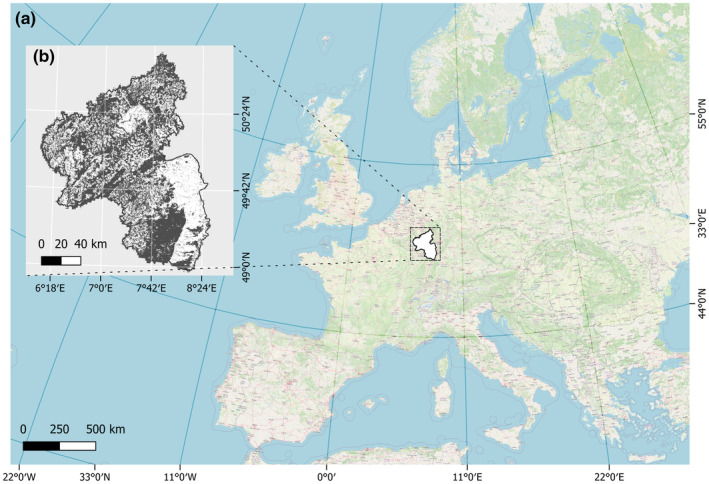 FIGURE 1
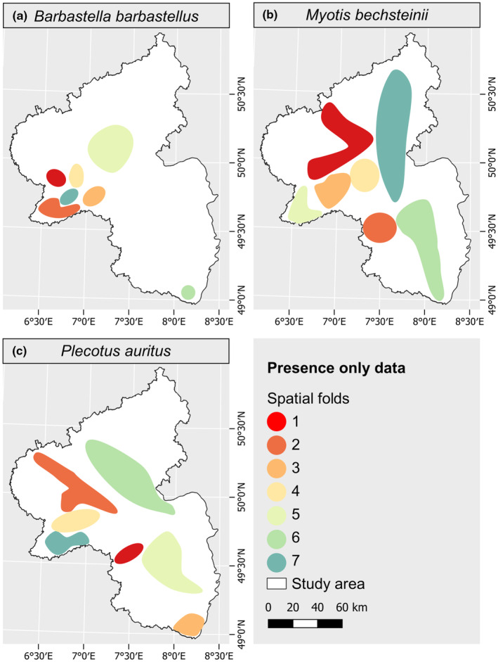 FIGURE 2
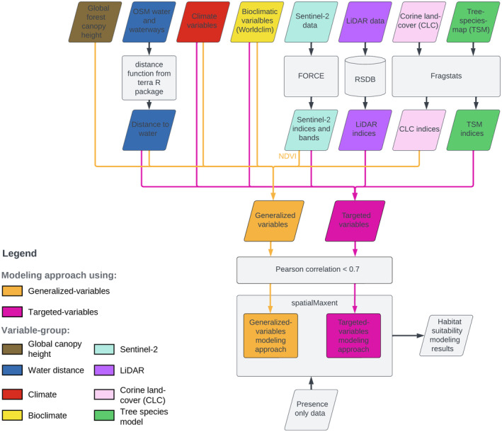 FIGURE 3
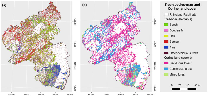 FIGURE 4
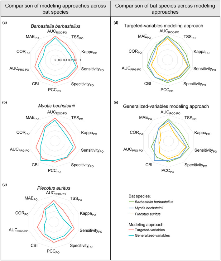 FIGURE 5
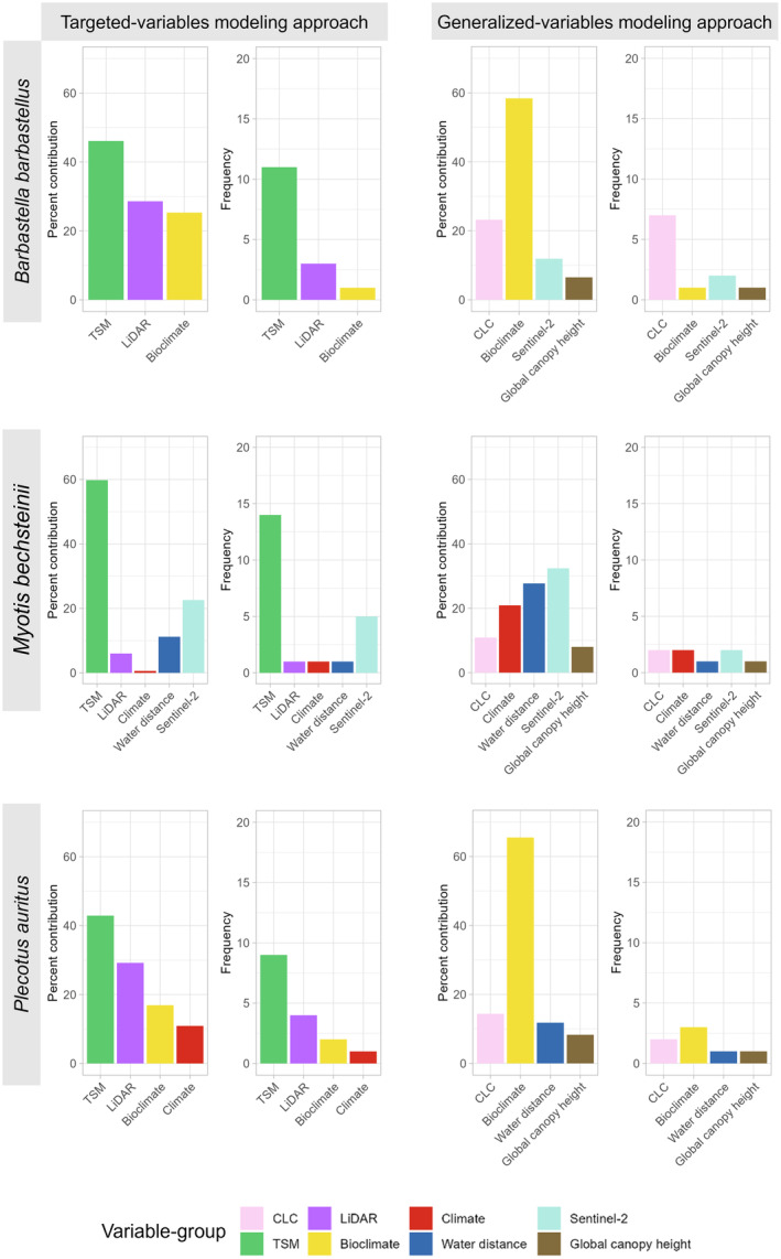 FIGURE 6
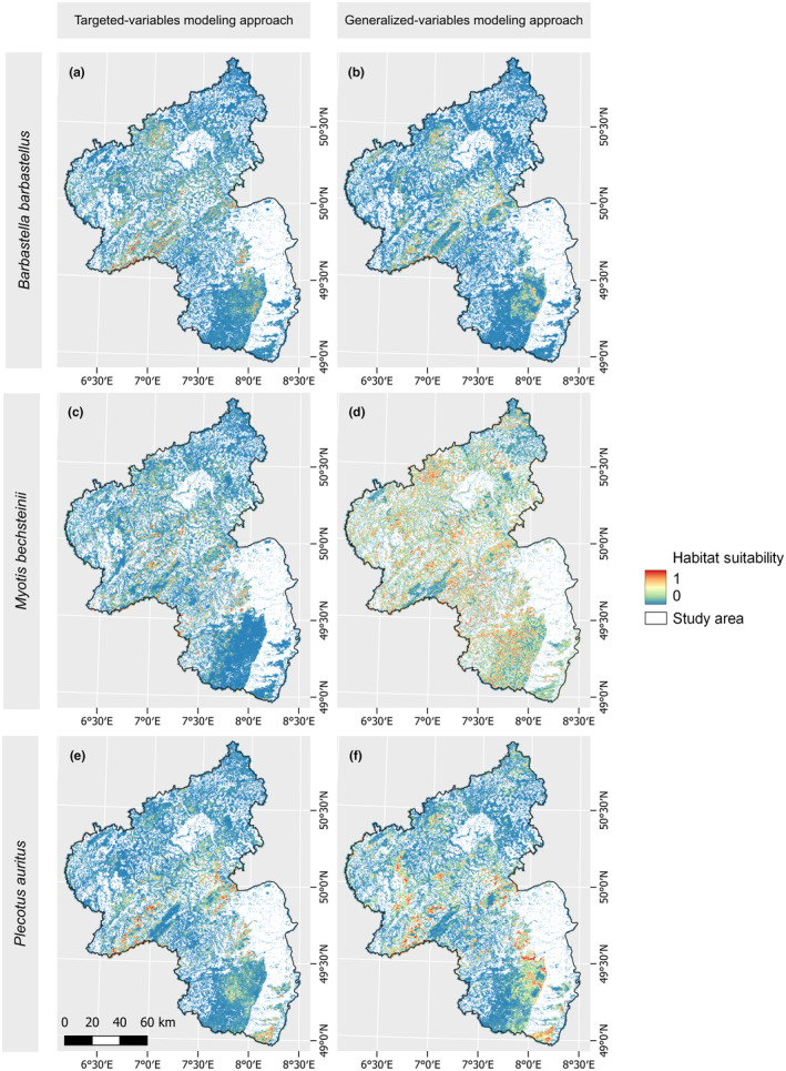 FIGURE 7
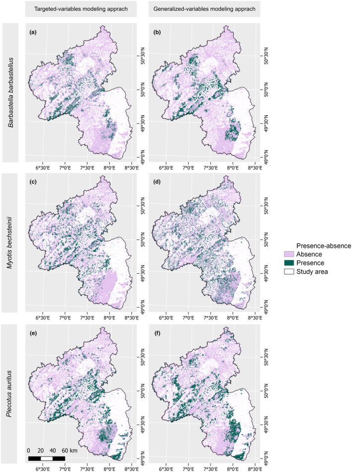 FIGURE 8
| Variable group | Targeted | Generalized |
|---|---|---|
| Land cover data | Tree species map (TSM) | Corine Land Cover (CLC) |
| Spectral satellite imagery | Monthly Sentinel‐2 time series with 10 bands and 19 indices | Monthly NDVI from Sentinel‐2 data |
| Vertical structure information | 29 indices calculated from LiDAR data | Global canopy height product |
| Climate data | Regional climate data on monthly, annual, and seasonal time scales | Regional climate data on monthly, annual, and seasonal time scales |
| Bioclimatic data | 19 bioclimatic variables | 19 bioclimatic variables |
| Distance to water | Distance to water based on OSM data | Distance to water based on OSM data |
| Species | Modeling approach | AUCROC‐PO | TSSPO | KappaPO | SensitivityPO | SpecitivityPO | PCCPO | CBI | AUCPRG‐PO | CORPO | MAEPO |
|---|---|---|---|---|---|---|---|---|---|---|---|
|
| Targeted variables |
|
|
|
|
|
|
|
|
|
|
| Generalized variables | 0.85 | 0.6 | 0.6 | 0.84 | 0.77 | 0.8 | 0.76 | 0.69 | 0.49 | 0.37 | |
|
| Targeted variables |
|
|
|
|
|
| 0.82 |
|
|
|
| Generalized variables | 0.78 | 0.49 | 0.49 | 0.73 | 0.76 | 0.74 |
| 0.57 | 0.48 | 0.37 | |
|
| Targeted variables |
|
|
|
|
|
|
|
|
|
|
| Generalized variables | 0.7 | 0.37 | 0.37 | 0.71 | 0.66 | 0.68 | 0.57 | 0.38 | 0.3 | 0.43 |
- —Hessian State Offensive for the Development of Scientific‐Economic Excellence (LOEWE)
- —Landesamt für Umwelt Rheinland‐Pfalz
Peer Reviews
No public reviews on file for this paper yet. If you reviewed it on a platform where reviews are public (OpenReview, ICLR, NeurIPS, ICML), you can paste yours below so the community can read it here.
Videos
No videos yet. Explain this paper in a talk, walkthrough, or lecture? Add one.
Taxonomy
TopicsWeb and Library Services · Mobile and Web Applications · Distributed and Parallel Computing Systems
INTRODUCTION
1
Species distribution modeling (SDM) and habitat suitability modeling (HSM) are commonly utilized for mapping species across diverse ecological fields (Franklin, 1995; Guisan & Zimmermann, 2000). For targeted nature conservation measures in particular, but also for the planning of interventions in the environment, it is paramount to map out valuable habitats for endangered species as precisely as possible. However, recent research has shown that models often exhibit poor performance in accurately predicting species distribution (Lee‐Yaw et al., 2022) and should therefore be treated with caution.
SDM and HSM involves the selection of appropriate environmental variables (Scherrer & Guisan, 2019). Traditionally, climate variables, such as bioclimatic data, have been widely employed for SDM and HSM (e.g., Amini Tehrani et al., 2020; Bandara et al., 2022; Bellamy et al., 2020; Cable et al., 2021; Luo et al., 2020; Raman et al., 2020; True et al., 2021; Wright et al., 2021). However, for the assessment of habitat suitability within the geographic range of a species (area of habitat (AOH); Brooks et al., 2019; Lumbierres et al., 2022), climate conditions are not necessarily decisive (Pearson et al., 2004). To model the AOH, factors beyond climate variables are essential. Studies have demonstrated that incorporating spectral remote sensing variables enhances SDM and HSM (Leitão et al., 2019; Randin et al., 2020; Regos et al., 2022).
In addition to climatic factors, human intervention in the landscape, such as creation and expanding of settlement, or agricultural activities, alters the environment, creates dispersal limitations, and disturbs biotic interactions to the extent that only a small portion of the area remains suitable as habitat for the species (Chauvier et al., 2021; Titeux et al., 2016). Land cover data have been employed in previous studies to incorporate environments shaped by human activities into the models. Typically, datasets such as the Corine Land Cover (CLC), which is readily available for all of Europe, are used, as it provides remote sensing‐derived land cover classes on a large scale (Abdi, 2013; Edman et al., 2011; Garrote et al., 2020; Posillico et al., 2004). However, the land use classes are only represented at a relatively coarse level of detail (e.g., three classes for forest). As the assumption behind HSM requires that environmental variables reflect the ecological niche of the target species (Araújo & Guisan, 2006), this level of detail is likely to be insufficient for precise modeling of habitat suitability for most species (e.g., Bradley & Fleishman, 2008; Cánibe et al., 2022; Gottwald et al., 2017; Mortelliti et al., 2007). Hence, HSM might require the utilization of more targeted classes in contrast to relying on widely available and therefore commonly utilized large‐scale land cover datasets.
In this study, we tested this hypothesis by comparing the influence of environmental variables that are representing the same information, but at different levels of detail (e.g., tree species composition vs. mixed, coniferous, and deciduous forest classes) on model performance and the resulting HSM maps for three forest‐dwelling bat species (Barbastella barbastellus, Myotis bechsteinii, and Plecotus auritus) in Rhineland‐Palatinate, Germany. A customized and targeted land cover dataset that provides forest habitat information at the tree species level for the entire federal state of Rhineland‐Palatinate, Germany (Bald et al., 2024) was used, in combination with high‐information remote sensing datasets such as light detection and ranging (LiDAR), also available for the entire federal state of Rhineland‐Palatinate, to optimally reflect the ecological requirements of the target species. We compared the results with those obtained when using more generalized spatial variables at a coarser level of detail that are typically used for HSM such as the CLC dataset.
For both variable sets, the same state‐of‐the‐art modeling workflow in Maxent (Phillips et al., 2006, 2017; Phillips & Dudík, 2008) that incorporates an automated variable selection and model tuning approach based on spatial cross‐validation was employed (Bald et al., 2023). Spatial cross‐validation was chosen due to recent studies highlighting its importance for model training, variable selection, and tuning, to prevent inflated performance metrics and overly complex models (Kattenborn et al., 2022; Meyer et al., 2018, 2019; Ploton et al., 2020; Roberts et al., 2017).
The objective of this study is to compare two distinct modeling approaches, one employing targeted variables, tailored to reflect the ecological requirements of the target species (Araújo & Guisan, 2006), and the other utilizing generalized variables commonly used in HSM, these are hereafter referred to as targeted variables modeling (TVM) approach and generalized variables modeling (GVM) approach.
MATERIALS AND METHODS
2
All data pre‐ and postprocessing were done in R version 4.1.2. For processing raster data, the R packages terra (version 1.7.3, Hijmans, 2023) and raster (version 3.6.3, Hijmans, 2022) were used. Additionally, the R package sf (version 1.0.7, Pebesma, 2018) was employed for processing vector data. The habitat suitability models were created with the software extension spatialMaxent (Bald et al., 2023).
Study area
2.1
The federal state of Rhineland‐Palatinate, covering a total area of 19,858 km^2^ in southwestern Germany, served as the study area (Figure 1). With approximately 42% of its area covered by forests (BMEL, 2018), Rhineland‐Palatinate is acknowledged as one of the regions in Germany with the highest abundance of forests. The low mountain ranges are largely characterized by spruce and beech, while Rhineland‐Palatinate also features a large amount of oak and pine forests (PEFC, 2015). Rhineland‐Palatinate is home to 22 species of bats, including the forest‐dwelling Bechstein's bat (Myotis bechsteinii), which has its main distribution in Germany and is listed as critically endangered on the German Red List (IUCN, 2016a; Meinig et al., 2020). The barbastelle bat (Barbastella barbastellus) is also classified as critically endangered and the brown long‐eared bat (Plecotus auritus) as endangered (IUCN, 2016b, 2023; Meinig et al., 2020).
Study area. (a) Location of the study area, the federal state of Rhineland‐Palatinate, in Europe, Germany. (b) Forest cover of the study area (dark shading indicates forest cover and light shading indicates no forest cover). Data: EEA (2022) and OpenStreetMap (2023).
Focusing on forest‐dwelling bat species, the study area was confined to Rhineland‐Palatinate's forested regions, defined by a forest mask derived from the Copernicus high‐resolution forest cover map (2018) with a spatial resolution of 10 m (EEA, 2022). The forest cover map was used to mask all environmental variables, which were resampled to 50 m spatial resolution as a compromise between fine spatial resolution and number of raster cells to be processed. All environmental variables were resampled to or calculated based on the forest mask.
Presence‐only data
2.2
The presence‐only data (occurrence records) used in this study consisted of the locations of roosting trees frequented by female individuals of the three species during their reproductive period, serving as their summer habitat, collected between 2014 and 2022. 138 presence points were available for Barbastella barbastellus, 366 for Myotis bechsteinii, and 151 for Plecotus auritus. The data were collected by the BFL (Büro für Faunistik und Landschaftsökologie, Rümmelsheim; BFL, 2023) as part of a data query addressing all stakeholders engaged in bat conservation initiatives within Rhineland‐Palatinate. Due to the close proximity of some roost trees, the points were thinned using the R package spThin (version 0.2.0, Aiello‐Lammens et al., 2015) to ensure a minimum distance of 50 m between them. The spThin algorithm is based on the concept of nearest neighbor distance (Aiello‐Lammens et al., 2015). This process aims to have no more than one record per raster pixel (50 m × 50 m) and therefore eliminates data duplicates. It resulted in 135 data points for Barbastella barbastellus, 285 points for Myotis bechsteinii, and 132 points for Plecotus auritus. For modeling purposes, these points were manually divided into seven spatial clusters, with each cluster serving as one cross‐validation fold in the modeling process (see Section 2.5), each representing a distinct spatial area (Figure 2). We opted for seven spatial folds to allow for the removal of two folds for testing purposes, while still enabling us to conduct five fold spatial cross‐validation.
Spatial folds delineating occurrence records for each bat species. Roosting sites of three bat species in Rhineland‐Palatinate, Germany, partitioned into spatial folds for validation and testing. Each fold encompasses multiple roosting sites.
Background points
2.3
Maxent is a presence‐only modeling method, but requires the inclusion of artificial background points for model training and validation (Phillips et al., 2006). These background points were distributed randomly across the entire study area, aimed at representing the whole spectrum of environmental predictor variables. In numerous studies, the number of background points used was 10,000 (e.g., Bandara et al., 2022; Kafash et al., 2022; Wright et al., 2021), which is the default setting for Maxent (Phillips et al., 2006). However, recent studies have shown that higher numbers of background points may be necessary for large study areas (Renner et al., 2015; Warton & Shepherd, 2010). As our study area covers 19,858 km^2^, we decided to use a total of 50,000 background points. They were created using the function randomPoints() from the R package dismo (version 1.3.9; Hijmans, Phillips, et al., 2022).
Environmental variables
2.4
A total of 754 environmental variables were used in this study, which involves a comparative analysis of two modeling approaches for each of the three bat species considered: one utilizing generalized variables and the other employing targeted variables (Figure 3). The full set of environmental variables consisted of eight different variable groups (Figure 3): Spectral remote sensing data from a Sentinel‐2 time series (ESA), indices derived from airborne LiDAR data (GeoBasis‐DE/LVermGeoRP, 2021), climate data (DWD Climate Data Center [CDC] 2014, 2023a, 2023b, 2023c, 2023d, 2023e, 2023f, 2023g), bioclimatic data (Fick & Hijmans, 2017), a global canopy height map produced with GEDI data (Potapov et al., 2021), indices derived from a tree species map (TSM; covering the six most important tree species in the study area; Bald et al., 2024; Figure 4), indices derived from CLC forest classes (EEA, 2018; Figure 4), and a raster showing the distance of each pixel to water in the study area (OpenStreetMap, 2023). Detailed information on the acquisition and processing of these variables is provided in the Appendix. The variables from different groups were incorporated into one or both of the two modeling approaches. In both modeling approaches, all variable groups were covered (Table 1), even though realistically, not all variable groups are used for most habitat modeling (e.g., often only climate data are used). Furthermore, we do not claim completeness regarding the variable groups used here. Depending on the species, other variable groups may also be of importance.
Habitat suitability modeling workflow. This flowchart outlines the comprehensive modeling process for three bat species, employing two modeling approaches with distinct sets of variables. Environmental variables from eight different variable groups, namely global canopy height data (Potapov et al., 2021), OpenStreetMap (OSM) waterways data (OpenStreetMap, 2023), climate data (DWD Climate Data Center [CDC], 2014, 2023a, 2023b, 2023c, 2023d, 2023e, 2023f, 2023g), bioclimatic variables from WorldClim (Fick & Hijmans, 2017), Sentinel‐2 satellite imagery (ESA), Light detection and ranging (LiDAR) data (GeoBasis‐DE/LVermGeoRP, 2021), Corine Land Cover (CLC) data (EEA, 2018), and variables derived from a tree species map (TSM; Bald et al., 2024) were used. Utilizing analytical tools such as Framework for Operational Radiometric Correction for Environmental Monitoring (FORCE; version 3.7.7, Frantz, 2019), Remote Sensing Database (RSDB; Wöllauer et al., 2020), and Fragstats (version 4.2; McGarigal et al., 2023), these inputs were processed to generate indices. The resulting variables were divided into a generalized and a more targeted stack of variables. These variables served as input for the modeling, where two models were created for each bat species. Variables that were part of the generalized variables modeling approach are displayed in orange. Variables that were part of the targeted variables modeling approach are displayed in pink. Variables can be part of both the generalized variables and the targeted variables modeling approach.
Tree species map and Corine Land Cover. (a) The six most common tree species in the study area are beech, Douglas fir, oak, spruce, pine, and other deciduous trees (Bald et al., 2024). (b) CLC forest classes used in the study: deciduous forest, coniferous forest, and mixed forest (EEA, 2018).
Targeted environmental variables
2.4.1
For the TVM the complete Sentinel‐2 time series, totaling 203 variables (“Sentinel‐2 data” in the Appendix) was employed. Furthermore, all 29 LiDAR indices (“LIDAR data” in the Appendix), 103 climate variables (“Climatic variables” in the Appendix), 19 bioclimatic variables (“Bioclimatic variables” in the Appendix), 265 tree species map variables (“Tree‐species‐map” in the Appendix), and the distance to water variable (“Distance to water” in the Appendix) were utilized. The data selected here as target variables were chosen to be more detailed than commonly used variables. However, this does not mean that other more detailed variables that were not considered here could not yield similar or even better results. For example, data on prey availability, such as maps of insect abundance (e.g., Partridge et al., 2020; Sierro & Arlettaz, 1997), may also be valuable.
In total, 620 variables were generated for the TVM. Pearson correlation analysis was performed to identify variables that demonstrated high similarity. Given that the modeling process utilized only the background points and not the complete environmental rasters, the correlation analysis was also conducted on the background points. Variables displaying a correlation exceeding 0.7 were excluded from further analysis to mitigate multicollinearity issues (Dormann et al., 2013; Zurell et al., 2020). This resulted in 111 variables that were used for the TVM (“Initial variable stack used for the targeted‐variables modeling approaches” in the Appendix).
Generalized environmental variables
2.4.2
The GVM approach involved a selection of variables commonly found in existing literature. Specifically, all 19 bioclimatic variables (“Bioclimatic variables” in the Appendix), and all 103 climate variables (“Climatic variables” in the Appendix) were incorporated, as they were among the most commonly used variables for SDM (e.g., Amini Tehrani et al., 2020; Bandara et al., 2022; Bellamy et al., 2020; Cable et al., 2021; Luo et al., 2020; Raman et al., 2020; True et al., 2021; Wright et al., 2021). If variables reflecting the three‐dimensional forest structure were utilized, these often involve canopy height data (e.g., Amini Tehrani et al., 2020; Raman et al., 2020). Therefore, the global forest canopy height product (“Global forest canopy height product” in the Appendix) was used as a predictor variable (Potapov et al., 2021). In terms of spectral data, normalized difference vegetation index (NDVI) often predominates for habitat modeling (e.g., Amini Tehrani et al., 2020; Kafash et al., 2022; Luo et al., 2020). Therefore, all NDVI variables from the time series (VI10 January, March, April, May, June, September, and October; “Sentinel‐2 data” in the Appendix) were included. Instead of class indices derived from the tree species map, the indices based on the CLC dataset (“Corine Land Cover” in the Appendix) were integrated. While the application of land cover information (e.g., Amini Tehrani et al., 2020; Bandara et al., 2022; Bellamy et al., 2020; Cable et al., 2021; Luo et al., 2020; Thomas et al., 2021; Wright et al., 2021) and/or landscape information via Fragstats or the R package landscape metrics is common in habitat modeling (e.g., Cable et al., 2021; Neubaum & Aagaard, 2022; Thomas et al., 2021), the highest resolution for forest classes typically extends no further than the categories provided by CLC, namely broadleaf, coniferous, or mixed forest (e.g., Amini Tehrani et al., 2020; Andersen et al., 2022; Bandara et al., 2022; Cable et al., 2021; Thomas et al., 2021; True et al., 2021). Therefore, the GVM approach incorporates all indices derived from the CLC dataset, amounting to 133 indices (compared to 265 for the tree species map variables with six classes for forest). Finally, the variable “distance to water” (“Distance to water” in the Appendix) was included, as similar variables based on vector datasets were commonly integrated (e.g., Amini Tehrani et al., 2020; Cable et al., 2021; Luo et al., 2020). The complete raster stack consisted of 263 variables. A Pearson correlation on all background points was calculated and variables with a correlation higher than 0.7 were removed. This resulted in 65 environmental variables used for the generalized variables habitat modeling (“Initial variable stack used for the generalized‐variables modeling approaches” in the Appendix).
Modeling with spatialMaxent
2.5
Identifying the optimal modeling method for SDM is challenging, as numerous studies comparing different approaches frequently yield conflicting results (Elith et al., 2006; Elith & Graham, 2009; Gao et al., 2023; Guisan et al., 2007; Hoffman et al., 2010; Oppel et al., 2012; Rahman et al., 2022; Valavi et al., 2022, 2023; Wisz et al., 2008). Some studies indicate favorable outcomes with random forest or ensemble models (Gao et al., 2023; Oppel et al., 2012; Rahman et al., 2022), while others demonstrate high performance for Maxent (Phillips et al., 2006) or boosted regression trees (Elith et al., 2006; Guisan et al., 2007; Wisz et al., 2008). Two comprehensive benchmark studies by Valavi et al. (2022, 2023) found that ensemble models (such as biomod2; Thuiller et al., 2009) only achieve satisfactory results when each model within the ensemble is meticulously tuned, validated, and tested. Another top performing method in these two benchmark studies was Maxent (Phillips et al., 2006, 2017; Phillips & Dudík, 2008), which is one of the most widely adopted techniques for modeling species distribution (Guillera‐Arroita et al., 2015). The varying performance of Maxent in such comparisons is likely due to the fact that Maxent only achieves good results when thorough tuning is conducted for each species (Merow et al., 2013; Morales et al., 2017).
SDM models frequently exhibit poor performance on spatially independent test data (Lee‐Yaw et al., 2022), often due to the neglect of properties inherent in spatial data (Bahn & McGill, 2012). For example, numerous studies have highlighted the importance of spatial validation, to avoid inflated evaluation metrics and suboptimal parameter selection (Bahn & McGill, 2012; Bald et al., 2023; Meyer et al., 2018, 2019; Ploton et al., 2020). Furthermore, hyperparameters of the models should be tuned for each species (Merow et al., 2013; Morales et al., 2017), using spatial validation to select the right parameters. The same applies to variable selection; it has been shown that using too many variables can lead to bias in the results (Irving et al., 2020; Wang et al., 2016; Williams et al., 2012). Moreover, better results were achieved when variables were selected automatically rather than manually by the modeler (Meyer et al., 2019; Yiwen et al., 2016). Additionally, variable selection must be based on a spatial validation method to generate reliable results (Bald et al., 2023; Meyer et al., 2018, 2019). As these functionalities are not yet all available for the aforementioned high‐performing ensemble models without substantial complexity, the software spatialMaxent (version 1.0.0; Bald et al., 2023) was used in this study. spatialMaxent is an extension for Maxent version 3.4.4 (Phillips et al., 2006) and allows the utilization of Maxent with a spatial cross‐validation, a variable selection and tuning of feature classes and regularization multiplier. Furthermore, spatialMaxent achieved better modeling results on a benchmark dataset of over 200 species than a more standardized version of Maxent, indicating that direct comparison between the two is not feasible (Bald et al., 2023).
The implemented variable selection was a forward variable selection (Meyer et al., 2019). In forward variable selection, the selection process begins by training a model for all possible combinations of two variables. The best two variables are selected, and one more model with one additional variable is trained for each remaining variable. The model with the best three‐variable combinations is retained. This process is repeated until no further improvement is observed by adding more variables. For additional details on forward variable selection, refer to Meyer et al. (2019).
Using spatialMaxent a total of six models were calculated, two for each bat species, one with the targeted variables and one with the generalized variables, including forward variable selection, forward feature selection and regularization multiplier tuning in steps of 0.5 from 0.5 to 7 and spatial cross‐validation.
Model comparison
2.6
In this study, two modeling approaches were compared: one employing targeted variables (see Section 2.4.1), and the other utilizing generalized variables (see Section 2.4.2). For each of the three bat species analyzed, two models were developed employing identical modeling workflows (see Section 2.5), differing only in their input variables. The TVM approach incorporated 111 variables, while the GVM approach comprised 64. Employing an automated variable selection method ensured that only the essential variables were retained (Meyer et al., 2018, 2019), therefore, the difference in the initial variable count should not influence the comparability of the models.
Evaluation
2.7
To evaluate the models, forward fold metric estimation (ffme; Bald et al., 2023), a variant of nested cross‐validation (Schratz et al., 2019) was employed. Two out of the seven spatial folds were consistently utilized for testing the models, while the remaining five folds were used for spatial five fold cross‐validation. This process was iterated for all possible combinations of two test and five training folds, resulting in the calculation of 21 models (7!/((7 − 2)! * 2!)) for model testing for each species and modeling approach. For all 21 models, several evaluation metrics were calculated and the mean value across all 21 models was used to assess the performance. To determine the best modeling approaches numerous metrics were utilized, aiming to minimize uncertainties associated with each individual metric (Lobo et al., 2008). In metrics requiring absence points, an equivalent number of background points as available presence points were randomly sampled. Following the recommendation of Yackulic et al. (2013), these metrics are labeled as presence‐only (PO), such as MAE_PO_ for mean absolute error.
Konowalik and Nosol (2021) recommend using the area under the receiver operating characteristics curve (AUC_ROC‐PO_) and the mean absolute error (MAE_PO_) for selecting the model with the best performance. Therefore, the MAE_PO_ was calculated using R package Metrics (version 0.1.4; Hamner & Frasco, 2018) and the AUC_ROC‐PO_ with the function evalSDM() from the R package mecofun (version 0.1.1; Zurell, 2020). Another commonly used metric in SDM is Kappa_PO_, which can be influenced by species prevalence; as an alternative, the true skill statistic (TSS_PO_) has been suggested (Allouche et al., 2006). We employ both metrics here to provide a comprehensive overview, and both were also calculated using the R package mecofun (version 0.1.1; Zurell, 2020). In their benchmark SDM study, Valavi et al. (2022) also used the area under the precision‐recall‐gain curve (AUC_PRG‐PO_) and Pearson correlation between observed and predicted values (COR_PO_). Therefore, we have also used these metrics for our study and calculated the AUC_PRG‐PO_ with the function calc_auprg() from the R package prg (version 0.5.1; Kull & Flach, 2023), as well as Pearson correlation using the R function cor() (R Core Team, 2023). There is only one commonly used metric available for evaluating the performance of SDM solely on presence data: the continuous Boyce index (CBI; Boyce et al., 2002). Therefore, this metric was also included and computed using the R package ecospat (version 3.5; Broennimann et al., 2023). Finally, we included three additional metrics, namely, Sensitivity_PO_, Specificity_PO_, and percent correctly classified (PCC_PO_) as they are commonly used in SDM according to Mouton et al. (2010). They were also calculated using the R package mecofun (version 0.1.1; Zurell, 2020).
To compare the habitat suitability maps of the TVM approach with the maps of the GVM approach, we utilized two metrics. The Pearson correlation, calculated with the layerCor() function from the terra R package (Hijmans, 2023), and the root mean square error (RMSE) were applied to assess map differences. Additionally, habitat suitability maps were transformed into presence–absence maps using the evalSDM() function from the R package mecofun (version 0.1.1; Zurell, 2020), with threshold selection based on maximizing the TSS_PO_ across all folds. We recognize that the method for generating presence–absence maps can influence results (Wilson et al., 2005). By consistently applying the same threshold selection method across all models, we ensure a valid comparison, aligning with our emphasis on only comparing the TVM approach and the GVM approach.
RESULTS
3
Performance of TVM and GVM approaches
3.1
For all three bat species researched in this study, the TVM approach consistently outperformed GVM approach across the majority of calculated metrics (Figure 5; Table 2). For Barbastella barbastellus and Plecotus auritus, the TVM approach performed better on all metrics (Figure 5a,c). For Barbastella barbastellus, the largest disparity among metrics was evident in COR_PO_, with a mean value of 0.65 for the TVM approach compared to 0.49 for the GVM approach (Figure 5a). For Plecotus auritus, the greatest difference was observed in the mean AUC_PRG‐PO_ metric, recording 0.66 for the TVM approach and 0.38 for the GVM approach (Figure 5c). The smallest difference between metrics for all bat species was found in mean MAE_PO_, where the difference between modeling approaches was less than 0.1 (Figure 5a–c). For the species Myotis bechsteinii, superior outcomes were evident for all metrics in the TVM approach, except for CBI (Figure 5b). The mean CBI was 0.92 for the GVM approach and 0.82 for the TVM approach. Among the targeted variable models of all the bat species, Barbastella barbastellus performed the best, followed by Myotis bechsteinii, and Plecotus auritus ranked the lowest (Figure 5d). In the generalized variable models, the pattern was similar, with only CBI for Myotis bechsteinii being better than the other two species (Figure 5e).
Comparison of model performance. Mean test results for all three bat species using both targeted variables and generalized variables modeling approaches. Figures (a) to (c) present individual bat species' metric results, comparing the two modeling approaches. Figures (d) and (e) provide a cross‐species comparison between targeted variables and generalized variables modeling approaches. The MAEPO is presented at a reversed scale to enhance readability. Note that comparing metrics to each other is not feasible, as they are on different scales. Only comparisons between different modeling approaches and species are possible for each metric. The axis ranges from 0 to 1 in steps of 0.2, as shown in (a). The direct comparison of modeling approaches for each bat species shows that, with the exception of one metric (CBI, Myotis bechsteinii), the targeted variables modeling approach consistently outperforms the generalized variables modeling approach (a–c).
Contribution of variable groups
3.2
A close analysis of the selected variables showed that, within the TVM approach, variables derived from the tree species map variable group make a notable contribution (Figure 6), collectively accounting for over 40% in each model. The targeted variable models of Plecotus auritus and Myotis bechsteinii had one of the tree species map variables among the first two most important variables (“Variable importance of all three bat species and two modeling approaches” in the Appendix, Figure A1). The targeted variable model of Barbastella barbastellus selected a variable from the tree species map variable group as the third most important variable (“Variable importance of all three bat species and two modeling approaches” in the Appendix, Figure A1). For all three bat species, the tree species map variables had also the highest number of selected variables. The models of Barbastella barbastellus and Myotis bechsteinii selected over ten variables from the tree species map variables, while only nine were chosen by the targeted variable model of Plecotus auritus. For the targeted variable model of Barbastella barbastellus and Plecotus auritus, the second most important variables belonged to the LiDAR variables. For both species, the LiDAR variables exhibited a contribution exceeding 20%, and were the second most influential variable group based on the number of selected variables, three variables were selected for Barbastella barbastellus, and four variables for Plecotus auritus. The targeted variable model for Barbastella barbastellus identified a variable from the bioclimatic category as the most crucial, although this was the only one selected from these variables group. In the targeted variable model for Myotis bechsteinii, the Sentinel‐2 variable group emerged as the second most important, with a total of five variables selected, collectively contributing 22.6%. Subsequently, a LiDAR variable, a climate variable, and the distance‐to‐water variable were also chosen.
Variable contribution analysis. Each bat species and modeling approach are represented with two plots. The right plot illustrates the cumulative percentage contribution of variables within each variable group. The left plot displays the frequency distribution (number of variables) within each variable group. For the left plot the sum of the percent contribution of the variable group to the model are on the y‐axis and the variable groups on the x‐axis. For the right plot the frequency, how often a variable from the variable group was chosen by the model is on the y‐axis and the variable group on the x‐axis. The variable groups are bioclimatic variables, climatic variables, Corine Land Cover (CLC) variables, distance to water variable, global canopy height variable, light detection and ranging (LiDAR) variables, Sentinel‐2 variables, and tree species map (TSM) variables.
In the GVM approach, it becomes apparent that the noteworthy contribution of the tree species map variable group in the TVM approach and its frequent selection could not be replaced by the variables of the CLC variable group (Figure 6). Instead, the bioclimatic variables contributed the highest for Barbastella barbastellus (58.4%) and Plecotus auritus (65.5%), while for Myotis bechsteinii, the Sentinel‐2 variables group was the most important one (32.4%). However, the generalized variable model for Barbastella barbastellus used only one bioclimatic variable while the variable group from which the most variables were selected was CLC, with 7 selected variables that contributed a total of 23.2%. The generalized variable model of Plecotus auritus selected three variables from the bioclimatic variable group, with the second most important variable group being CLC, both in terms of the number of variables (two variables) and contribution (14.4%). The contribution of the individual variable groups was more evenly distributed for Myotis bechsteinii. The highest contribution, comprising 32.4%, came from the Sentinel‐2, with two variables selected from this group. Additionally, two variables each were selected from the CLC (10.9%) and climate (20.9%) variable groups. However, the variable distance to water had the next highest contribution of 27.7%. The variable group global canopy height was consistently included in all generalized variable models. The contribution in all generalized variable models showed that bioclimatic variables were not very often selected but with a very strong contribution, similar to the distance to water variable. The CLC variable group, similar to the tree species map variable group in the TVM approach, was frequently selected, but with lower contributions that often lagged behind those of the Sentinel‐2 and climate variables.
Comparisons of modeling approaches for presence–absence and habitat suitability maps
3.3
In this section, we undertake two comparisons. First, we analyze the agreement between the habitat suitability maps produced by the TVM approach with those generated by the GVM approach, examining each bat species individually. Furthermore, we compare the suitable areas of the presence–absence maps that were generated through thresholding the habitat suitability maps, specifically evaluating the differences between the TVM approach and the GVM approach.
When comparing the habitat suitability maps of the two modeling approaches directly (Figure 7), Plecotus auritus exhibited the highest agreement between the two maps, with a Pearson correlation of 0.45. The maps of Myotis bechsteinii ranked at a similar level, as indicated by a Pearson correlation of 0.42. Barbastella barbastellus performs least favorably in this regard, with a Pearson correlation of 0.36. However, examining the RMSE values reveals that the differences of the two modeling approaches is higher for Myotis bechsteinii, with an RMSE value of 0.33, while Barbastella barbastellus and Plecotus auritus have RMSE values of 0.18 and 0.21, respectively.
Habitat suitability maps. Maps showing the habitat suitability of the forested areas for all three bat species and the targeted variables (left) and generalized variables (right) modeling approach. Values close to 0 (blue) indicate low habitat suitability while values closer to 1 (red) indicate high habitat suitability. Study area is in white.
In the habitat suitability maps, thresholding was applied to generate presence–absence maps (refer to Section 2.7). Upon examining the suitable areas delineated in the presence–absence maps (Figure 8), it becomes evident that, for the TVM approach, fewer areas were determined as suitable compared to the GVM approach. The largest difference in the predicted suitable area is for Myotis bechsteinii, where the disparity in suitable area between the TVM approach (2133.26 km^2^) and the GVM approach (2677.59 km^2^) is 544.33 km^2^. Both modeling approaches predict the largest suitable area for Plecotus auritus compared to the other two bat species, with 2370.13 km^2^ for the TVM approach and 2755.48 km^2^ for the GVM approach. The smallest difference in suitable area between the TVM approach (1498.45 km^2^) and the GVM approach (1716.75 km^2^) is observed for Barbastella barbastellus, with a difference of 218.31 km^2^, and this species also had the smallest overall predicted area in both modeling approaches.
Presence–absence maps. Showing presence–absence maps of the forested areas for all three bat species using the targeted variables (left) and generalized variables (right) modeling approach. Study area is in white. Differences in mapped area between targeted variables and generalized variables modeling approach for the species are as follows: Myotis bechsteinii 544.33 km2, Plecotus auritus 385.35 km2, and Barbastella barbastellus 218.31 km2.
DISCUSSION
4
To evaluate how variables at a high level of detail affect model performance and resulting HSM maps, we contrasted the performance of targeted variables containing information on forest structure (LiDAR), and tree species composition with environmental variables that reflect the same landscape features but with less detail on the landscape composition, such as CLC dataset or a canopy height model.
The large contribution of tree species map based variables, along with structural variables (LiDAR; Barbastella barbastellus and Plecotus auritus) and spectral remote sensing time series variables (Myotis bechsteinii), underscores the importance of targeted variables that reflect local species habitat conditions. That remote sensing variables contribute to improved results in HSM has previously been addressed (Leitão et al., 2019; Leyequien et al., 2007; Randin et al., 2020; Regos et al., 2022). However, often the focus is on the utilization of spectral remote sensing data (e.g., Amini Tehrani et al., 2020; Kafash et al., 2022; Luo et al., 2020). In contrast, the frequent selection of LiDAR variables by the TVM approach suggests that structural data enhances model performance compared to relying solely on spectral data or canopy height information. Given the widespread availability of LiDAR data, particularly in Europe, their inclusion should be more frequently considered in HSM. The importance of high‐information spectral remote sensing data (Oeser et al., 2020) was further confirmed in our study (second most important variable group for Myotis bechsteinii).
The GVM selected CLC variables for all three bat species but their lower contribution, compared to tree species map variables in the TVM, indicates a limited ability to capture nuanced habitat requirements essential for precise HSM. This is also supported by Mortelliti et al. (2007) who previously highlighted the inadequacy of forest classes in the CLC dataset for accurately describing the habitat of specialized forest‐dwelling species. However, the modeling of species with a broad ecological niche may not necessarily benefit from the utilization of targeted land‐cover variables.
The large differences in the habitat suitability maps, with a highest agreement in Pearson correlation between TVM and GVM of 0.45, further emphasize the need to proceed with caution when selecting environmental variables for HSM. These findings are consistent with prior research, showing discrepancies in model outcomes with varying variables (Bucklin et al., 2014; Syphard & Franklin, 2009).
Nonetheless, the predicted suitable areas align with species niche width, designating Barbastella barbastellus as the most threatened as well as most habitat‐demanding and Plecotus auritus as the least demanding among the three bat species. The GVM consistently predicted larger suitable areas than the TVM. This aligns with recent studies indicating an overestimation of species' ranges compared to their actual AOH (Jetz et al., 2008; Rondinini et al., 2005). The observed limitations of GVM in accurately delineating AOH emphasize the need for more targeted approaches to habitat suitability mapping, as bias introduced by the overestimation of the AOH can heavily influence conservation outcomes (Jetz et al., 2008).
The results of HSM are always associated with high uncertainties and should therefore be treated like a hypothesis (Jarnevich et al., 2015). Nevertheless, they have potential as informative tools for habitat conservation and management strategies. For example, the maps created in this study could be utilized in spatial planning endeavors, such as determining suitable locations for wind farms and infrastructure projects (Gaultier et al., 2020; Roscioni et al., 2013). Before commencing on‐site evaluations of such projects, the locations can be chosen to minimize habitat suitability in the project area. Subsequently, an on‐site investigation can be conducted. This approach can enhance the likelihood that none of the three endangered species are found during the on‐site assessment and thus shorten planning time and costs (Roscioni et al., 2013). Additionally, our findings have implications for forest management. LiDAR data were often selected by the models as important variables, indicating that forests with high structural complexity are favored by all three bat species (Figure 6; Froidevaux et al., 2016). Furthermore, these three forest‐dwelling bat species demonstrate a preference for deciduous forests, with a high proportion of oak (“Variable importance of all three bat species and two modeling approaches” in Appendix). Such findings highlight the necessity of integrating these considerations into statewide forest management planning, particularly when decisions concern areas with high habitat suitability, as there is a risk of further habitat loss for these species.
Further research, testing alternative modeling methods beyond Maxent, will be important to reinforce and generalize the findings of this study. In summary, the integration of targeted variables, including tree species classification and remote sensing data (spectral and LiDAR data), has enhanced HSM for forest‐dwelling bat species in Rhineland‐Palatinate, Germany. Furthermore, it was shown that the choice of environmental variables heavily influences habitat suitability maps. This result underlines the necessity of selecting spatial variables with the best possible approximation to the ecological requirements of the target species, even if this can involve a considerable effort in data preparation. Despite the great potential of HSM for species conservation in practical application, our results suggest that habitat suitability maps should be used cautiously, recognizing their limitations and dependency of the results on choice of environmental variables. It is important to acknowledge the uncertainties associated with these maps (Jarnevich et al., 2015), urging users to interpret them with skepticism and employ complementary data sources for more robust decision‐making in conservation efforts.
AUTHOR CONTRIBUTIONS
Lisa Bald: Conceptualization (equal); formal analysis (equal); investigation (equal); methodology (equal); validation (equal); visualization (lead); writing – original draft (equal); writing – review and editing (equal). Jannis Gottwald: Conceptualization (equal); formal analysis (equal); investigation (equal); methodology (equal); supervision (equal); validation (equal); visualization (supporting); writing – original draft (equal); writing – review and editing (equal). Jessica Hillen: Writing – review and editing (equal). Frank Adorf: Writing – review and editing (equal). Dirk Zeuss: Supervision (equal); writing – review and editing (equal).
CONFLICT OF INTEREST STATEMENT
The authors have no conflict of interest to declare.
The reference list from the paper itself. Each links out to its DOI / PubMed record.
- 1Abdi, A. (2013). Integrating open access geospatial data to map the habitat suitability of the declining corn bunting (Miliaria calandra). ISPRS International Journal of Geo‐Information, 2(4), 935–954. 10.3390/ijgi 2040935 · doi ↗
- 2Aiello‐Lammens, M. E. , Boria, R. A. , Radosavljevic, A. , Vilela, B. , & Anderson, R. P. (2015). sp Thin: An R package for spatial thinning of species occurrence records for use in ecological niche models. Ecography, 38(5), 541–545. 10.1111/ecog.01132 · doi ↗
- 3Allouche, O. , Tsoar, A. , & Kadmon, R. (2006). Assessing the accuracy of species distribution models: Prevalence, kappa and the true skill statistic (TSS). Journal of Applied Ecology, 43(6), 1223–1232. 10.1111/j.1365-2664.2006.01214.x · doi ↗
- 4Amini Tehrani, N. , Naimi, B. , & Jaboyedoff, M. (2020). Toward community predictions: Multi‐scale modelling of mountain breeding birds' habitat suitability, landscape preferences, and environmental drivers. Ecology and Evolution, 10(12), 5544–5557. 10.1002/ece 3.6295 32607173 PMC 7319251 · doi ↗ · pubmed ↗
- 5Andersen, B. R. , Mc Guire, L. P. , Wigley, T. B. , Miller, D. A. , & Stevens, R. D. (2022). Habitat associations of overwintering bats in managed pine forest landscapes. Forests, 13(5), 803. 10.3390/f 13050803 · doi ↗
- 6Araújo, M. B. , & Guisan, A. (2006). Five (or so) challenges for species distribution modelling. Journal of Biogeography, 33(10), 1677–1688. 10.1111/j.1365-2699.2006.01584.x · doi ↗
- 7Bahn, V. , & Mc Gill, B. J. (2012). Testing the predictive performance of distribution models. Oikos, 122(3), 321–331. 10.1111/j.1600-0706.2012.00299.x · doi ↗
- 8Bald, L. , Gottwald, J. , & Zeuss, D. (2023). spatial Maxent: Adapting species distribution modeling to spatial data. Ecology and Evolution, 13(10), e 10635. 10.1002/ece 3.10635 37881225 PMC 10594137 · doi ↗ · pubmed ↗