Balancing the Encoder and Decoder Complexity in Image Compression for Classification
Zhihao Duan, Adnan Faisal Hossain, Jiangpeng He, Fengqing Zhu

TL;DR
This paper explores how to balance encoder and decoder sizes in image compression to improve classification performance and flexibility.
Contribution
The paper introduces a feature compression-based method that allows adjustable trade-offs between compression rate, accuracy, and model size.
Findings
Encoder and decoder sizes have a complementary relationship in image compression for classification.
The proposed method achieves competitive results on ImageNet with greater flexibility than existing methods.
Abstract
This paper presents a study on the computational complexity of coding for machines, with a focus on image coding for classification. We first conduct a comprehensive set of experiments to analyze the size of the encoder (which encodes images to bitstreams), the size of the decoder (which decodes bitstreams and predicts class labels), and their impact on the rate-accuracy trade-off in compression for classification. Through empirical investigation, we demonstrate a complementary relationship between the encoder size and the decoder size, i.e., it is better to employ a large encoder with a small decoder and vice versa. Motivated by this relationship, we introduce a feature compression-based method for efficient image compression for classification. By compressing features at various layers of a neural network-based image classification model, our method achieves adjustable rate, accuracy,…
Genes, proteins, chemicals, diseases, species, mutations and cell lines named across the full text — each resolved to its canonical identifier and authoritative record.
Click any figure to enlarge with its caption.
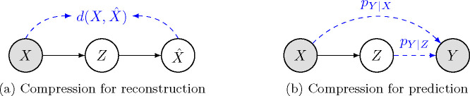 Figure 1
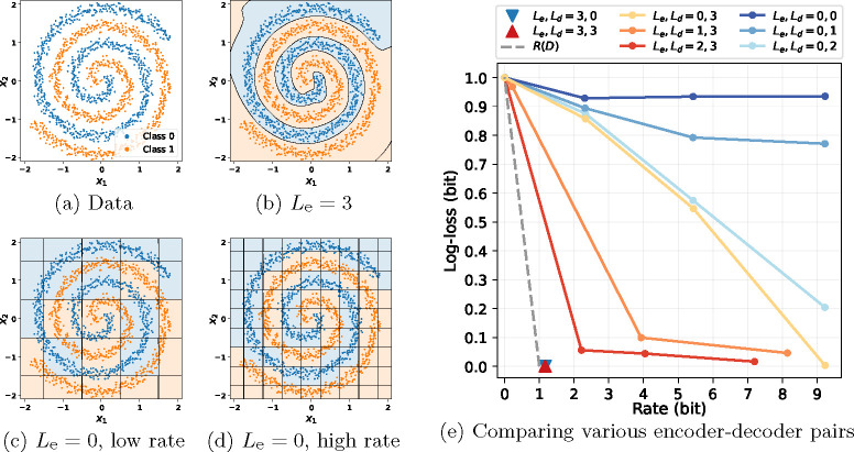 Figure 2
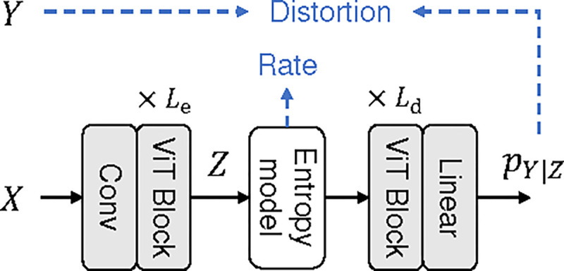 Figure 3
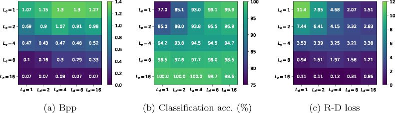 Figure 4
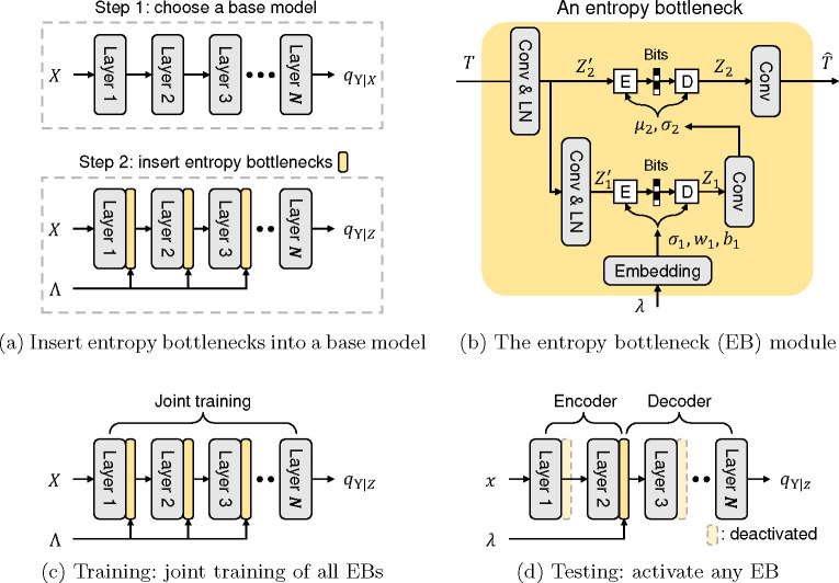 Figure 5
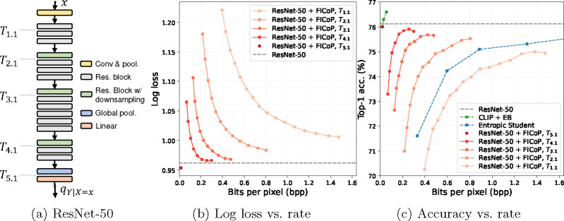 Figure 6
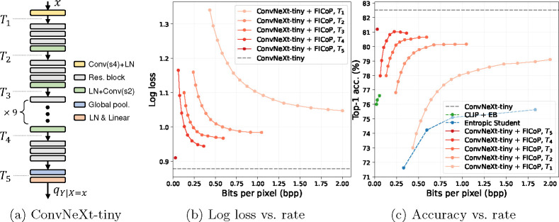 Figure 7
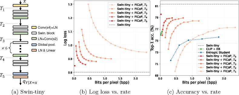 Figure 8
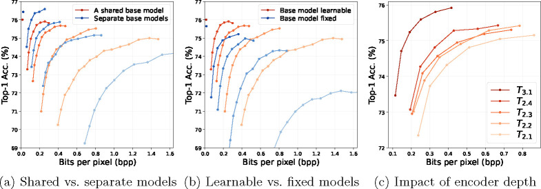 Figure 9
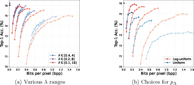 Figure 10
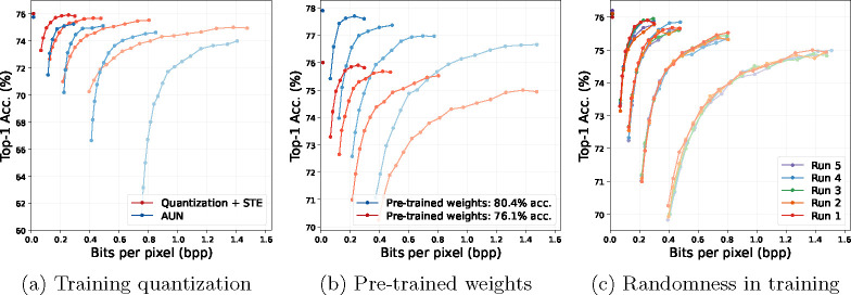 Figure 11
 Figure 12
 Figure 13
Peer Reviews
No public reviews on file for this paper yet. If you reviewed it on a platform where reviews are public (OpenReview, ICLR, NeurIPS, ICML), you can paste yours below so the community can read it here.
Videos
No videos yet. Explain this paper in a talk, walkthrough, or lecture? Add one.
Taxonomy
TopicsGenerative Adversarial Networks and Image Synthesis · Advanced Image Processing Techniques · Advanced Data Compression Techniques
Introduction
1
Data compression is a fundamental problem in information theory as well as many real-world applications. Recently, coding for machines emerges as a promising scheme in data compression, in which case one aims to represent data using as few bits as possible while retaining high prediction accuracy for downstream vision tasks. Coding for machine approaches have already many potential applications such as edge-cloud computing [1–3], privacy-preserving communication [4, 5], and the Internet of Things [6, 7].
Most existing research on coding for machines focuses on the rate-accuracy trade-off, where rate measures the average number of bits per sample produced by the encoder, and accuracy measures the downstream task (e.g., ImageNet classification [8]) prediction accuracy on the decoder side. This is a natural extension of the classical rate-distortion trade-off in lossy compression, and various prior works have studied coding for machine problems based on rate-distortion theory [9–11]. In particular, Dubois et al. [9] have theoretically proved that, for certain tasks, it is possible to achieve a high prediction accuracy with an extremely low rate compared to reconstruction-oriented compression.
Yet what is feasible in theory may not always be achievable in practice. Rate-distortion theory, which describes the best possible rate-distortion (or rate-accuracy in our context) trade-off, assumes an unbounded encoder and decoder family. However, many practical applications involve constraints on computational resources (e.g., for mobile and wearable devices), which limit the choice of encoder and decoder architectures. Such constraints render the theoretical rate-accuracy bounds inapplicable, calling for a more practical analysis of coding for machine performance under computational constraints.
Motivated by this, we first study the rate-accuray trade-off in coding for machines under computational constraints on the encoder and decoder. Our analysis reveals that such constraints would greatly impair the rate-accuracy trade-off, leading to a three-way trade-off between rate, accuracy, and computational complexity. Targeting this trade-off, we propose an end-to-end learning framework for adjusting these three quantities using a single neural network model, which has not been achieved by existing methods.
To summarize, we make the following contributions to the study of coding for machines: (Sec. 3) We empirically investigate the impact of encoder/decoder size on coding for machine performance. Our analysis reveals a complementary relationship between the encoder and decoder sizes, as well as a three-way trade-off between rate, distortion, and encoding complexity; (Sec. 4 and 5) We propose a novel method for adjusting this three-way trade-off that requires only a single neural network model. Experiments show that our method achieves comparable rate-distortion-complexity performance with existing methods while being much more flexible for deployment.
Preliminaries
2
This section briefly reviews the theoretical foundations of lossy compression. Readers familiar with rate-distortion theory and coding for machines may skip this section.
Rate-distortion theory.
Let denote the source data variable. In lossy compression for reconstruction (Fig. 1a), also referred to as coding for human vision, the goal is to represent using as few bits as possible, from which one can obtain a good reconstruction . The distortion is quantified by a function measuring the difference between and . Given a distortion threshold , the minimum rate (i.e., average number of bits per sample when compressing an i.i.d. sequence of ) required to achieve is given by the information rate-distortion function [12]:
where is mutual information. Note that the reconstruction need not be in the same space as the source . In coding for machines, for example, the reconstruction is often a prediction target instead of the original data.
Rate-distortion in coding for machines.
Let be a joint distribution, where denotes data, and is the prediction target. In compression for prediction (Fig. 1b), we again want to represent using a low-rate representation, but on the decoding side, the objective now is to infer instead of reconstructing . Prior research has applied the rate-distortion theory to coding for machines in various ways [9–11]. Among them, a representative approach [9] is to regard the compressed representation as the “reconstruction” and adopt the following distortion function:
where is the KL divergence. Intuitively, Eq. (2) measures how well a representation can be used to predict , compared to predicting using . This distortion equals the best-case classification log loss and simulates the prediction error in many downstream tasks. With this distortion, the information rate-distortion function becomes:
which follows from Theorem 2 of [9]. Intuitively, the distortion threshold determines the maximum information loss regarding allowed during encoding. When , no information loss is allowed, and the encoder must retain all task-related information in the representation . In this case, the minimum achievable rate equals , and the compression is lossless in the sense that predicting from is as good as predicting from . When , the encoder is allowed to discard a subset of , and the minimum achievable rate decreases accordingly.
Assumptions.
We consider neural network-based (as opposed to hand-crafted) encoders and decoders, the complexity of which can be controlled by tuning the number of network layers and the number of dimensions per layer. We apply elementwise uniform quantization and use factorized entropy models [13] for . We consider image classification as the downstream prediction task. More general settings (e.g., vector quantization and other downstream tasks) are left to future work.
Rate-Distortion under Computational Constraints
3
We perform two experiments (Sec. 3.1 and Sec. 3.2) to study the impact of encoder and decoder size on the R-D trade-off in coding for machines. In both experiments, we assume that the encoder and decoder are neural networks accompanied by uniform scalar quantization, following the non-linear transform coding framework [14]. Computational constraints are thus imposed by varying the neural network depth (number of layers) and width (number of dimensions per layer). Sec. 3.3 discusses the observations and motivates our proposed method for image coding for machines (Sec. 4).
Experiment: 2-D datapoint classification
3.1
We considers a toy problem of 2-D datapoint compression for classification, shown in Fig. 2a. The data is 2-D, the label is binary with equal probability, and the difference between the two classes is an angular shift in polar coordinates. In this experiment, the rate is measured by bits per datapoint, and the distortion is measured by classification log loss (also known as the cross-entropy loss).
According to Eq. (3), we know that one could achieve no distortion with bit per datapoint (when compressing long sequences). To verify this, we train a neural compressor [14] with a powerful encoder and decoder, both of which are MLPs with 3 hidden layers. Its R-D performance is shown as the red triangle marker in Fig. 2e. We observe that this particular compressor successfully achieves a performance close to , i.e., zero distortion with a rate close to 1 bit.
Then, we reduce the encoder and decoder sizes by decreasing the number of hidden layers and dimensions. Let denote the number of hidden layers in the encoder, and the number of hidden layers in the decoder. We try with various combinations of , and show the results in Fig. 2e. We make the following observations based on the results:
Given a powerful encoder, restricting the decoder does not hurt R-D: we keep and reduce to 0 (i.e., a linear decoder). This configuration is shown as the blue triangle mark in Fig. 2e. In this case, restricting the decoder size does not affect the R-D performance, indicating that given a powerful encoder, a simple decoder suffices to make accurate predictions.Given a powerful decoder, restricting the encoder increases rate: we gradually reduce from 3 to 0 while keeping . Note that refers to a simple elementwise uniform quantizer. Results are shown as the yellow and red curves in Fig. 2e. We see that to achieve the same distortion, the rate increases as the encoder size decreases. Note that even weak encoders are able to achieve near-zero distortion, as long as given a sufficiently high rate (e.g., when , ).For a weak encoder, restricting the decoder increases distortion: we keep and decrease from 2 to 0, shown as the blue curves in Fig. 2e. This increases the distortion at all rates, indicating that a powerful decoder is necessary to make accurate predictions when using weak encoders.
To better understand the behavior of the encoders with different number of layers, we visualize their quantization regions in Fig. 2b for , and Fig. 2c and 2d for . We see that the large encoder (Fig. 2b) encodes only task-related information, which is the polar angular shift in this toy problem, and data points with the same label are quantized to the same code. In contrast, the small encoder (Fig. 2c and 2d) is not able to extract the task information due to its restricted capacity, and extra bits are used to code task-irrelevant information, i.e., datapoint positions in Cartesian coordinates.
This toy problem of 2-D classification gives intuitions about the functionality of the encoder and decoder with different sizes (and thus different expressive power). Next, we conduct experiments for natural images to verify our observations.
Experiment: CIFAR-10 classification
3.2
This section considers a more realistic scenario where we use vision transformer-based [15] encoders and decoders to compress the CIFAR-10 dataset for classification. CIFAR-10 [16] is a natural image classification dataset that is widely used in machine learning research. It contains 60,000 RGB images (50,000 for training, 10,000 for testing) of ten different object categories, and each image has 32 × 32 pixels. We use a vision transformer-based model (shown in Fig. 3) to compress the images and make predictions from the compressed representation. The encoder and decoder sizes are controlled by their number of ViT blocks, denoted by and , respectively. Rate is measured by bits per pixel (bpp), distortion is measured by the cross-entropy loss, and the Lagrange multiplier used is . We train the model for 100k iterations with batch size 256, learning rate 0.001, Adam optimizer [17], and cosine learning rate schedule. We apply various combinations of and , and the experimental results are presented in Fig. 4. The main observations are summarized as follows.
Increasing the encoder size significantly reduces bpp, but increasing the decoder size does not.
This can be observed in Fig. 4a. For a fixed encoder size , increasing the decoder size leads to an unchanged (for ) or worse bpp (e.g., for ). However, for a fixed , increasing from 1 to 16 reduces bpp from around 1.0 to around 0.07. In other words, the rate is highly (negatively) correlated with , but it is approximately independent of . This is largely expected, as the rate is independent of the decoder when given the data source and the encoder^1^.
Increasing either the encoder size or the decoder size improves the classification accuracy.
This can be seen from Fig. 4b. When fixing (first row in the figure), increasing from 1 to 16 improves the accuracy from 77.0% to 99.9%. When fixing (first column in the figure), a similar trend can be observed. This suggests that a powerful end-to-end model (i.e., the encoder concatenated with the decoder) is necessary to make accurate predictions. Note that increasing the model size does not always improve classification accuracy. For example, when , increasing the decoder size from 4 to 16 decreases the accuracy from 100.0% to 98.6%. This is presumably because training larger models typically requires more training iterations and data [18], which is not the case in our simple setting (we use the same training recipe for all models).
A complementary relationship exists between the encoder and decoder sizes.
Looking at Fig. 4c, we see that the best choice of for is , indicating that a powerful decoder is necessary to achieve good R-D performance when the encoder is weak. Contrarily, is one of the best choices when , indicating that a simple decoder is sufficient when the encoder is powerful. If we list the best pairs for each (i.e., we compute argmin for the rows in Fig. 4c), we obtain , , , , . That is, as the encoder size increases, the best choice of the decoder size decreases.
Desired properties of a practical method
3.3
Our observations in previous sections suggest several insights for designing a flexible and efficient method for compression for prediction. First, since there is a multi-way trade-off among rate, distortion, and encoder capacity, a flexible method should be capable of operating at various combinations of these factors to accommodate different application scenarios. Second, the method may take advantage of the complementary relationship between the encoder and decoder. For example, when the encoder is powerful enough, one needs only a simple decoder to produce an accurate prediction. Otherwise, a complex and powerful decoder is needed. In the following section, we propose a method that satisfies these properties.
Adjusting the Rate, Prediction Accuracy, and Encoder-Decoder Complexity Using a Single Model
4
We present an end-to-end framework for image compression for prediction. Our method, FICoP (Flexible Image Compression for Prediction), uses only a single model to achieve adjustable rate, distortion, and encoding/decoding complexity, making it a flexible method for practical applications.
Overview
4.1
Fig. 5 overviews our approach. Suppose an existing neural network model takes data as input, produces a (first-order) Markov chain of features, and predicts the conditional label distribution (we use to distinguish it from the true data distribution ). Our method is a plug-and-play extension that takes the base model and inserts entropy bottlenecks (EBs) in between its layers (Fig. 5a). Each EB can be viewed as a splitting point that divides the model into an encoder and a decoder , and at test time (Fig. 5d), one can freely choose which EB to activate. By splitting the model in such a way, we can control the encoding complexity and, at the same time, take care of the complementary relationship between the encoder and decoder. For example, activating an EB at the early layer results in a small encoder and a large decoder, and vice versa.
For each EB, the training objective is to minimize the rate-distortion Lagrangian:
where denotes the entropy of the discrete latent representation estimated by a neural entropy model [13], the KL term is the distortion, and is a Lagrange multiplier that trades off rate and distortion. A key contribution in our method is to optimize Eq. 4 for multiple EBs at a range of using a single end-to-end training process (Fig. 5c). Note that we use in the loss function as well as pass it to the model as an input.
The entropy bottleneck (EB) module
4.2
Fig. 5b shows the entropy bottleneck module. It follows the Hyperprior structure [13], a two-layer VAE architecture commonly used for image compression. The compressed representation contains two components and with an auto-regressive prior . We describe the details and highlight the differences from the original design as follows.
A lightweight bottleneck architecture.
Unlike in Ballé et al. [13] where a stack of CNN layers is used, we use single convolutional layers for all transformations. Our objective is to keep the small size of each EB so that we can insert multiple EBs into any existing model without significantly increasing the overall model size. Non-linearity is achieved by layer normalization [19] operations, which has been shown effective in image compression [20–22]
Quantization with straight-through gradient estimator.
As the standard practice, we quantize and using elementwise uniform quantization before invoking the entropy coding algorithm. However, as opposed to the additive uniform noise in [13], we apply hard quantization during training as well, and the gradients are approximated using the straight-through estimator (STE) [23, 24]. Although STE is shown sub-optimal in compression for reconstruction [25, 26], we find that STE is better than additive uniform noise in our setting (Appendix B.2).
Probablistic models and variable-rate compression.
We model the prior for and using the discretized Gaussian distribution [27]:
where is a function of (through an embedding layer), and are functions of (through a convolutional layer), as shown in Fig. 5b. The embedding layer consists of a sinusoidal positional encoding [28] followed by an MLP, following [29]. We achieve rate-adaptive quantization [30, 31] by applying an affine transform and its inverse to before and after nearest integer rounding, respectively:
where is the variable before quantization, and the affine parameters are produced by the embedding layer. This adaptive quantization is also applied for , which we omit in Fig. 5b for simplicity. Equation (5) effectively conditions the prior on , and Eq. (6) conditions the encoder on , allowing us to control the rate-distortion by varying the input to the model.
Training objective
4.3
Given a base model employed with multiple EBs, we train them jointly in a single training process (Fig. 5c). Specifically, let denote the index for the EBs, and be a pre-defined distribution over the indices, which we choose to be uniform in our experiments. At each training iteration, we activate the k-th EB and deactivate the others for a sampled from . To achieve variable-rate training, we also randomly sample from a distribution throughout training. This is then used in the loss function as well as to condition the EBs. In our experiments, we choose to be a log-uniform distribution with a range of [0.1,16], and we discuss these choices of hyperparameters in Appendix B.1.
Formally, the training objective is to minimize the following loss w.r.t. all model parameters (including the base model and all EBs):
where the first term corresponds to rate, and the second corresponds to distortion.
Experiments
5
Without otherwise specified, we use the ResNet-50 [32] as the base model in this section. We show that our method generalizes well to other model architectures in Appendix B.
Dataset and metrics.
We use the 1,000-class ImageNet dataset [8] for training (train split) and evalutation (val split). In evaluation, all images are resized to 224 × 224 pixels, and the rate is measured in terms of bits per pixel (bpp) after resizing. The distortion is estimated by the log loss (also known as the cross-entropy loss) of the model prediction w.r.t. the ground truth label. We also report the top-1 classification accuracy, which is more interpretable. All metrics are computed for each image in the val set and then averaged across the entire val set.
Augment ResNet-50 with FICoP.
ResNet-50 contains five stages (excluding the first convolutional layer), each of which contains multiple blocks. We take ResNet-50 with pre-trained weights as the base model and insert EBs to the splitting points shown in Fig. 6a. The splitting points are referred to as , where is the stage index, and is the block index in the stage (the indices start from 1). The resulting model is referred to as ResNet-50 + FICoP and is trained on ImageNet train split for 160k iterations with a batch size of 256. For to , we train the EBs with . For , we found that the model is not sensitive to and the rate is always close to zero, so we only train it at . The full details of training hyperparameters are given in Appendix A.
Validating the rate-distortion-complexity trade-off
5.1
Fig. 6b shows the rate-distortion (R-D) results of ResNet-50 + FICoP operating at each splitting point, and each of them produces a separate R-D curve. The encoding complexity for the case of all splitting points is reported in Table 1. We also show results for the original ResNet-50 as a reference.
Comparing the R-D curves in Fig. 6b, we observe that a deeper splitting point (which consumes higher encoding complexity) achieves better R-D performance. This is expected by our analysis, as a more powerful encoder is able to compress away more task-irrelevant information, thus reducing the rate for the same distortion. Note that when the encoding complexity approaches that of the entire ResNet-50, i.e., at , the log loss converges to the one of the original ResNet-50 with a near-zero rate, which can be viewed as approaching the information function.
Comparing ResNet-50 + FICoP with existing methods
5.2
Existing methods.
We consider several related works as baselines. To our best knowledge, no existing method is able to achieve a rate-distortion-complexity trade-off using a single model as in ours, so a strictly fair comparison is not possible. We briefly describe these approaches as follows:
Dubois et al. [9] uses CLIP [33] together with an entropy bottleneck as the encoder and an MLP as the decoder. We refer to this method as CLIP + EB. Its setting differs from ours in that (a) CLIP is trained on image-text pairs instead of ImageNet, and (b) the method operates at only high encoding complexity.Matsubara et al. [3] uses a lightweight CNN encoder and a trunacted ResNet-50 decoder with knowledge distillation techniques applied during training. The method is referred to as Entropic Student. In their setting, one needs to train multiple models to operate at different rates, and only low encoding complexity is supported.
Fig. 6c shows the accuracy-rate results of our method compared to the baseline methods, and Table 1 shows the corresponding encoding complexities. The Entropic Student method employs a lightweight encoder (around 0.47 GFLOPs) and thus achieves a much lower accuracy-rate curve than CLIP + EB (around 4.4 GFLOPs). Our method, however, is able to adjust the encoding complexity to control the accuracy-rate trade-off. In the low complexity regime, ResNet-50 + FICoP at and achieves similar accuracy-rate curves as Entropic Student, and in the high complexity regime, ResNet-50 + FICoP at achieves a comparable accuracy-rate curve as CLIP + EB. This demonstrates the flexibility and effectiveness of our approach in controlling the rate-distortion-complexity trade-off. Note that the accuracy-rate curves are not always monotonic because the method is trained to optimize the log loss, which does not always translate into classification accuracy.
FICoP with various base model architectures
5.3
FICoP with ConvNeXt [34].
To verify that our approach generalizes well to various model architectures, we choose a modern convolutional neural network architecture, ConvNeXt, as the base model. We apply FICoP to ConvNeXt-tiny, a lightweight version of ConvNeXt that achieves 82.5% top-1 accuracy on ImageNet, and show the results in Fig. 7. In the figure, Fig. 7a shows the model architecture and the layers in which we insert EBs, Fig. 7b show the distortion-rate results, and Fig. 7c show the accuracy-rate results. We observe a rate-distortion-complexity trade-off, which is consistent with our previous analysis. Furthermore, since ConvNeXt is a more powerful base model than ResNet-50, it leads to a significant performance boost when compared to the baseline methods.
FICoP with Swin-Transformer [35].
We also apply our approach to a Transformer architecture, Swin-Transformer, and show the results in Fig. 8. The observations are consistent with previous experiments, showing that our approach works well with Swin-Transformer and outperforms the baseline methods. We thus conclude that FICoP is a general approach that can be applied to various image classification model architectures.
Experimental analysis
5.4
We investigate our method by ablating its components. All other settings are the same as in the previous section.
Impact of joint training multiple entropy bottlenecks (EBs).
As our approach trains one shared base model jointly with multiple EBs, a natural question is how its performance differs from the one of training a separate base model for each EB. We thus train a separate ResNet-50 model for each EB at , and we refer to it as “separate base models” as shown in Fig. 9a. We observe that using a shared base model achieves comparable performance (better for low encoding complexity but worse for high encoding complexity) with multiple independent models while saving the parameters and training time by a factor of 5, as the latter needs five models in total.
A learnable base model is better than a fixed one.
Several prior methods also insert EBs into a pre-trained base model but keep the base model parameters fixed [1, 36, 37]. This approach has the advantage of allowing one to add new EBs incrementally without affecting the existing ones. We implement this strategy using our EBs and show the results in Fig. 9b. Compared to our joint training approach, it leads to worse accuracy-rate performance, especially in the low complexity regime, suggesting that it is important to finetune the base model such that it can adapt to the EBs.
Downsampling improves the accuracy-rate trade-off.
To understand how each ResNet-50 blocks contribute to the accuracy-rate performance, we place an entropy bottleneck after each block from to and show the results in Fig. 9c. The features at have the same dimension, while the feature at is 2 times smaller due to downsampling in the ResNet block. We again observe that a deeper entropy bottleneck achieves a better accuracy-rate trade-off. Interestingly, the accuracy-rate curve of is much better than that of . This is presumably because downsampling removes the dimensions that contain the irrelevant information and thus can largely improve the rate-distortion performance.
Related Work
6
Image/video coding for machines.
The most related works to our method are those on split computing [1, 36–39], where a pre-trained model is split into two parts and deployed on different devices, and the intermediate feature is compressed and then transmitted. However, to our knowledge, none of the existing works achieves end-to-end training of multiple splitting points as in ours. Several works considered compression for prediction under encoding complexity constraints [3, 40, 41], but the complementary relationship between encoder complexity and decoder complexity is not exploited. Other works design specific methods for particular applications such as video compression [42], privacy-preserving compression [4, 43], scalable coding [2, 44, 45], and the Internet of Things [6], which are orthogonal and can be combined with our method.
Impact of computational constraints in data compression.
In applications such as video compression, it is widely known that the encoding computational complexity can largely impact the rate-distortion trade-off [46–48]. For example, in modern video codecs such as VVC [49], requiring a fast encoding speed can lead to up to more than 30% rate increase [50]. This is consistent with our observation in compression for prediction. Nevertheless, techniques developed for image/video compression cannot be directly applied to our case due to the different nature of the two problems.
Information theory and compression in learning.
The objective of coding for machines resembles the one in information bottleneck methods [51–53], except that the latter does not require entropy coding. Thus, our study on the encoder/decoder complexity also applies to the information bottleneck methods. Several existing works also investigate the impact of computational constraints on information theory. Xu et al. [54] and Kleinman et al. [55] consider the amount of usable information between variables under constraints. A more related work is Harell et al. [10], where the authors prove that post-training compression of a deeper feature in a fixed model is better in terms of rate-distortion. Our paper explores the case where the base model is trainable, which is complementary to Harell et al. [10].
Conclusion
7
We have extended the rate-distortion trade-off in coding for machines to incorporate computational constraints. In particular, we show that a more powerful encoder leads to better rate-accuracy performance, and we reveal a complementary relationship between the required encoder size and the decoder size to achieve good performance. Experimental results have confirmed the existence of a three-way trade-off between rate, distortion, and model complexity, as well as showing the proposed method is advantageous over earlier methods in practical situations.
Limitations and future work.
An important assumption in our method is that in the base model, the model’s input-feature-output forms a Markov chain, which is not true for models with hierarchical features and skip connections [56, 57]. Also, we only consider image classification as the downstream task in this work. Future work could investigate more general cases, e.g., machine vision tasks such as image segmentation, human vision tasks such as image denoising and inpainting, and a combination of both [58].
The reference list from the paper itself. Each links out to its DOI / PubMed record.
- 1Choi H. & BajićI. V. Deep feature compression for collaborative object detection. Proceedings of the IEEE International Conference on Image Processing 3743–3747 (2018).
- 2Duan L., Liu J., Yang W., Huang T. & Gao W. Video coding for machines: A paradigm of collaborative compression and intelligent analytics. IEEE Transactions on Image Processing 29, 8680–8695 (2020).10.1109/TIP.2020.301648532857694 · doi ↗ · pubmed ↗
- 3Matsubara Y., Yang R., Levorato M. & Mandt S. Supervised compression for resource-constrained edge computing systems. Proceedings of the IEEE/CVF Winter Conference on Applications of Computer Vision 923–933 (2022).
- 4Azizian B. & BajićI. V. Privacy-preserving feature coding for machines. Picture Coding Symposium 205–209 (2022).
- 5Chen W.-N., Song D., Ozgur A. & Kairouz P. Privacy amplification via compression: Achieving the optimal privacy-accuracy-communication trade-off in distributed mean estimation. ar Xiv preprint ar Xiv:2304.01541 (2023).
- 6Shlezinger N. & BajićI. V. Collaborative inference for ai-empowered iot devices. IEEE Internet of Things Magazine 5, 92–98 (2022).
- 7Chamain L. D., Qi S. & Ding Z. End-to-end image classification and compression with variational autoencoders. IEEE Internet of Things Journal 9, 21916–21931 (2022).
- 8Deng J. Imagenet: A large-scale hierarchical image database. Proceedings of the IEEE Conference on Computer Vision and Pattern Recognition 248–255 (2009).