Interpretation of coefficients in segmented regression for interrupted time series analyses
Yongzhe Wang, Narissa J. Nonzee, Haonan Zhang, Kimlin T. Ashing, Gaole Song, Catherine M. Crespi

TL;DR
This paper explains how different ways of setting up segmented regression models can lead to different interpretations of the same data in interrupted time series analysis.
Contribution
The paper clarifies the differences in coefficient interpretation between two common segmented regression parametrizations in ITS analysis.
Findings
Both parametrizations represent the same model but differ in coefficient interpretation.
The immediate intervention effect is estimated differently depending on the parametrization used.
Researchers should be cautious when interpreting coefficients and calculating intervention effects.
Abstract
Segmented regression, a common model for interrupted time series (ITS) analysis, primarily utilizes two equation parametrizations. Interpretations of coefficients vary between the two segmented regression parametrizations, leading to occasional user misinterpretations. To illustrate differences in coefficient interpretation between two common parametrizations of segmented regression in ITS analysis, we derived analytical results and present an illustration evaluating the impact of a smoking regulation policy in Italy using a publicly accessible dataset. Estimated coefficients and their standard errors were obtained using two commonly used parametrizations for segmented regression with continuous outcomes. We clarified coefficient interpretations and intervention effect calculations. Our investigation revealed that both parametrizations represent the same model. However, due to…
Genes, proteins, chemicals, diseases, species, mutations and cell lines named across the full text — each resolved to its canonical identifier and authoritative record.
Click any figure to enlarge with its caption.
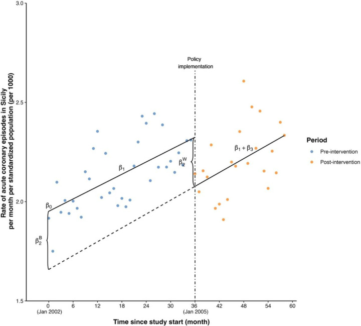 Figure 1
Peer Reviews
No public reviews on file for this paper yet. If you reviewed it on a platform where reviews are public (OpenReview, ICLR, NeurIPS, ICML), you can paste yours below so the community can read it here.
Videos
No videos yet. Explain this paper in a talk, walkthrough, or lecture? Add one.
Taxonomy
TopicsMental Health Research Topics · Statistical Methods and Bayesian Inference
Background
The interrupted time series (ITS) design is an increasingly popular quasi-experimental design that is used to estimate the effectiveness of an intervention when a randomized trial is not feasible.(1–7) In an ITS design, observations are collected in a time series over a study period that includes intervals both before and after the introduction of an intervention, and these observations are contrasted to estimate the intervention’s effectiveness. ITS designs have been used widely in health services research, for example, in the evaluation of health policies and health care quality improvement interventions in real-world settings. (2, 8–14)
The most widely used method of analyzing data from an ITS design study is segmented regression.(1, 2, 4–6, 15, 16) Segmented regression, also known as piecewise regression or broken-stick regression, is a method in regression analysis in which a series of observations is partitioned into intervals and a separate line segment is fit to each interval. The theoretical framework for estimating segmented regression dates back to the work of Quandt.(17, 18) The use of segmented regression for ITS dates back to its application in evaluating cross-sectional time series experiments in psychology.(19)
There are two common parametrizations for segmented regression applied to ITS analyses, that of Bernal et al.(6, 7) and that of Wagner et al.(4) Superficially, these two parametrizations appear similar, but they have important differences that impact the estimation of intervention effects, raising concerns about the potential for misinterpretation of results.(20) This paper investigates the two different parametrizations and their interpretations and illustrates the differences in interpretation by applying them to a real data set. (7)
Methods
Parametrizations of Segmented Regression
To explain the two common parametrizations of segmented regression for ITS, we consider the setting of a single interrupted time series collected from one unit (for example, a single clinic) with a continuous outcome variable.(3, 7) The key features of the model equation are a variable for continuous time, a binary indicator denoting the presence of an intervention, and an outcome measure.(1–3, 6, 7, 14, 15, 21) Let represent continuous time measuring the duration since the study’s initiation, starting from 0, and let denote the time at which the intervention is introduced. represents a binary indicator denoting the presence or absence of an intervention at time , equal to 0 for and 1 for . Let denote the continuous outcome as measured at time .
Bernal’s parametrization involves regressing the outcome on , and their interaction.(6, 7, 19, 22–25) Bernal’s parametrization(7) is:
In this parametrization, is the intercept in the pre-intervention interval and represents the mean outcome level at the inception of the study is the slope during the pre-intervention interval and represents the mean change in the outcome for a one unit increase in time. For the post-intervention interval, is the intercept and is the slope. Note that represents the outcome level at time 0 if we extrapolated the post-intervention regression line backwards in time. The coefficients and represent the differences in intercept and slope between the pre- and post-intervention intervals. Thus, this model allows for different linear regression models (different intercepts and different slopes) during the pre-and post-intervention intervals.
Two different aspects of an intervention effect can be captured with this segmented regression model.(4, 5, 21, 26, 27) One aspect is a change in the mean level of the outcome at time , corresponding to an immediate effect of the intervention on the outcome. The other aspect is the change in slopes from pre- to post-intervention, which represents a longer-term, gradual effect of the intervention on the outcome. In Bernal’s parametrization, the gradual effect corresponds to the change in slopes, which is in Eq. (1). However, the immediate effect does not correspond to the difference in intercepts .(4, 28) Rather, the immediate effect is the difference in means between the pre- and post-intervention models at the start of the intervention at time , which can be formulated as:
Hence in Bernal’s parametrization, is the difference in intercepts between the pre-and post-intervention models, that is, the vertical difference between the two regression lines at time 0, and the immediate effect is given by .
The parametrization of segmented regression advanced by Wagner is the same as Bernal’s parametrization except for the interaction term.(4) In Wagner’s parametrization, the interaction is the product of the binary intervention indicator and the time elapsed since the intervention’s implementation, . The model is:
Under this parametrization, the intercept and slope of the pre-intervention model are the same as for Bernal, but the intercept and slope of the post-intervention model are and , respectively. Thus, the two parametrizations differ in the parametrization of the intercept of the postintervention model. The difference in intercepts between the pre- and post-intervention models is . For intervention effects, represents the gradual effect, as it does in Bernal’s parametrization. However, the immediate effect, quantified as the mean change in levels at time , is given by:
Consequently, in this parametrization, captures the difference in means at the start of the intervention’s implementation. Thus when researchers use Wagner’s parametrization, the immediate effect can be directly extracted from .
It is important to highlight that the intercept and slope coefficients for the pre-intervention models in both parametrizations are the same. Additionally, the post-intervention slopes are the same, being represented by in both equations (2) and (4). The intercept terms of the two parametrizations are different: in Eq. (2) and in equation(4) . Assuming the post-intervention intercepts under the two parametrizations are equivalent, we can find that:
Hence, despite the differences between the two parametrizations, they should give the same estimate of the immediate effect of the intervention. In the next section, we show the alignment between the two parametrizations through the analytical expressions of the estimated coefficients. We summarize the interpretation of coefficients and intervention effects under the two different parametrizations in Table 1.
Estimated Coefficients
As observed, the parametrizations of segmented regression proposed by Wagner et al. and Bernal et al. have different model equations but correspond to the same pre- and post-intervention models. The two parametrizations also lead to different design matrices. The design matrix for Bernal’s parametrization is
where the upper part of the matrix represents the pre-intervention period, and the lower part represents the post-intervention period. We assume that there are and observations in the pre- and post-intervention periods, respectively, for a total of observations. The design matrix for Wagner’s parametrization is
Using design matrices or , we can obtain the ordinary least squares estimates of regression coefficients by solving the normal equations, obtaining where is the vector of the outcome variable. The covariance matrix for can be obtained as where represents the estimated residual, calculated as where indicates the number of columns in the design matrix. We will show the estimates of and in ordinary algebra rather than matrix algebra.
The estimates of , and take the forms
where represents the post-intervention slope such that . The summations to and to represent the summation over observations from the pre- and postintervention periods, respectively. Under both parametrizations, represents the mean outcome at study initiation and serves as the intercept in the pre-intervention model, represents the pre-intervention slope, and represents the difference in slopes between the pre-and post-intervention models. Note that and use only information from the pre-intervention period while uses observations from each period to estimate a period-specific slope and then takes the difference. The estimated variances of these coefficients are
The estimates of values for the two different parametrizations are:
where represents the post-intervention intercept under Bernal’s parametrization such that corresponds to the difference in intercepts between the pre- and post-intervention models. On the other hand, corresponds to the difference in the mean outcome at the time of intervention implementation. The estimated variances for for the two parametrizations are
Standard errors are obtained as the square root of the variances. For estimates of linear combinations of coefficients, such as and , the covariance between and is also needed to obtain the standard error. We omit this formula. All standard errors can be calculated in standard software.
Results
Illustration
We illustrate the differences in the two parametrizations using a dataset provided by Barone-Adesi et al. (29) and analyzed by Bernal et al.(7) The objective of Bernal et al.’s study was to assess the effectiveness of a policy that banned smoking in all indoor public places in Sicily, Italy. The policy implementation began in January 2005. The researchers adopted an ITS design and collected data between 2002 and 2006 on the standardized rates of acute coronary episodes (ACE) in Sicily per month. The standardized ACE rates were computed by dividing the monthly frequency of ACE hospital admissions in Sicily by the agestandardized population per person-year. We expressed the outcome as standardized ACE rates per 1000. There were 36 and 22 observations of standardized ACE rates in the pre- and post-intervention periods, respectively. Our focus is on illustrating the two parametrizations rather than providing a detailed analysis of these data, as was done by Bernal et al.(7). Hence, we do not present a complete analysis.
Table 2 displays estimated coefficients and intervention effects and standard errors calculated as described in previous sections. Figure 1 displays the fitted model. The supplementary materials include implementation details with code. is the intercept of the pre-intervention model and corresponds to the standardized rate of ACE per 1000 in January 2002, estimated as 1.95 (SE 0.05). is the slope of the pre-intervention model and indicates that the standardized rate of ACE per 1000 was increasing an estimated 0.01 units (SE 0.002) per month during this interval. At the time of intervention onset, it is estimated that the standardized rate of ACE per 1000 had dropped by 0.25 units (SE 0.08), corresponding to an immediate intervention effect; the decrease was statistically significant . Thereafter, the standardized ACE rate per 1000 continued to increase at an estimated rate of 0.01 per month (SE 0.004). The difference in slopes before and after intervention onset was not significantly different from zero, indicating no evidence of a gradual intervention effect.
The difference in estimates of between the two parametrizations of segmented regression is noteworthy. Figure 1 visually illustrates the difference between two estimated values. corresponds to the difference in the fitted outcome value at the time of intervention onset between the pre- and postintervention models (immediate effect), represented as the vertical distance between the two regression lines at that time point. In contrast, is the difference in intercepts between the pre- and postintervention models. In this dataset, the two quantities have similar values. This is because there is little difference in slopes between the pre- and post-intervention intervals. In data in which the two slopes are different, we would expect to see a greater difference between these two values.
Discussion
In our investigation of the two common parametrizations of segmented regression for ITS, we verified that the coefficients for baseline outcome level, pre-intervention trend, and difference in slopes pre- and postintervention onset are the same for both parametrizations. However, the interpretation of the coefficient for the binary intervention indicator differs between the two parametrizations. Under Wagner’s parametrization, this coefficient captures the difference in mean outcome between the pre- and postintervention models at the time of intervention implementation, indicating the change-in-level or immediate effect. Under Bernal’s parametrization, this coefficient is not the immediate effect but rather captures the difference in the intercept between the pre- and post-intervention models. Unfortunately, this coefficient has sometimes been misinterpreted in the literature.(28, 30–40)
When employing Bernal’s parametrization in segmented regression, it is important to recognize that the immediate effect should be calculated as a combination of two coefficients, as we have described. Conversely, when applying Wagner’s parametrization, the coefficient associated with the binary intervention indicator can be used as an estimate of the immediate effect and to get the difference in intercepts, one needs to use a combination of two coefficients. Thus, Bernal’s parametrization is more convenient for computing the difference in intercepts, while Wagner’s parametrization is more convenient for immediate effects. Users can choose between these parametrizations to tailor their estimates. Regardless of the chosen parametrization, both approaches yield the same pre- and post-intervention models.
Both parametrizations have limitations. They both hypothesize an outcome change immediately after intervention implementation and a linear change over time both before and after the intervention implementation. However, these assumptions might not accurately represent the dynamics of an ITS study; for example, intervention effects can exhibit lagged impacts. In such cases, one can consider alternative parametrizations that incorporate delayed effects or include a transition period between preintervention and post-intervention periods.(6, 16) Numerous technical issues related to segmented regression, such as autocorrelation, seasonality, and heterogeneity, have been addressed in existing literature.(1, 2, 4, 5, 15, 16, 22) By applying segmented regression and selecting appropriate parametrizations, users can employ tailored tools to mitigate technical issues based on the specifics of their data.
Conclusion
In conclusion, two common segmented regression parametrizations in ITS analysis represent the same model, yielding identical pre- and post-intervention models but distinct coefficient interpretations. Immediate intervention effect calculations differ between parametrizations, while gradual intervention effect calculations remain consistent. Both parametrizations for segmented regression can be employed as analytical approaches for ITS design, provided the specific nuances and interpretations of the coefficients are understood and explained.
The reference list from the paper itself. Each links out to its DOI / PubMed record.
- 1Ramsay CR, Matowe L, Grilli R, Grimshaw JM, Thomas RE. Interrupted time series designs in health technology assessment: lessons from two systematic reviews of behavior change strategies. Int J Technol Assess Health Care. 2003;19(4):613–23.15095767 10.1017/s 0266462303000576 · doi ↗ · pubmed ↗
- 2Hategeka C, Ruton H, Karamouzian M, Lynd LD, Law MR. Use of interrupted time series methods in the evaluation of health system quality improvement interventions: a methodological systematic review. BMJ Global Health. 2020;5(10):e 003567.33055094 10.1136/bmjgh-2020-003567 PMC 7559052 · doi ↗ · pubmed ↗
- 3Kontopantelis E, Doran T, Springate DA, Buchan I, Reeves D. Regression based quasi-experimental approach when randomisation is not an option: interrupted time series analysis. BMJ. 2015;350.10.1136/bmj.h 2750 PMC 446081526058820 · doi ↗ · pubmed ↗
- 4Wagner AK, Soumerai SB, Zhang F, Ross-Degnan D. Segmented regression analysis of interrupted time series studies in medication use research. J Clin Pharm Ther. 2002;27(4):299–309.12174032 10.1046/j.1365-2710.2002.00430.x · doi ↗ · pubmed ↗
- 5Gebski V, Ellingson K, Edwards J, Jernigan J, Kleinbaum D. Modelling interrupted time series to evaluate prevention and control of infection in healthcare. Epidemiol Infect. 2012;140(12):2131–41.22335933 10.1017/S 0950268812000179 PMC 9152341 · doi ↗ · pubmed ↗
- 6Bernal JL, Soumerai S, Gasparrini A. A methodological framework for model selection in interrupted time series studies. J Clin Epidemiol. 2018;103:82–91.29885427 10.1016/j.jclinepi.2018.05.026 · doi ↗ · pubmed ↗
- 7Bernal JL, Cummins S, Gasparrini A. Interrupted time series regression for the evaluation of public health interventions: a tutorial. Int J Epidemiol. 2017;46(1):348–55.27283160 10.1093/ije/dyw 098PMC 5407170 · doi ↗ · pubmed ↗
- 8Sears JM, Haight JR, Fulton-Kehoe D, Wickizer TM, Mai J, Franklin GM. Changes in early high-risk opioid prescribing practices after policy interventions in Washington State. Health Serv Res. 2021;56(1):49–60.33011988 10.1111/1475-6773.13564 PMC 7839645 · doi ↗ · pubmed ↗