CRouting: Reducing Expensive Distance Calls in Graph-Based Approximate Nearest Neighbor Search
Zhenxin Li, Shuibing He, Jiahao Guo, Xuechen Zhang, Xian-He Sun, Gang Chen

TL;DR
CRouting is a novel routing strategy that significantly reduces distance computations in graph-based approximate nearest neighbor search, enhancing efficiency with minimal modifications to existing algorithms.
Contribution
It introduces CRouting, a plugin that exploits high-dimensional angle distributions to bypass unnecessary distance calculations in graph-based ANNS methods.
Findings
Reduces distance computations by up to 41.5%.
Increases queries per second by up to 1.48×.
Applicable to HNSW and NSG graph indexes.
Abstract
Approximate nearest neighbor search (ANNS) is a crucial problem in information retrieval and AI applications. Recently, there has been a surge of interest in graph-based ANNS algorithms due to their superior efficiency and accuracy. However, the repeated computation of distances in high-dimensional spaces constitutes the primary time cost of graph-based methods. To accelerate the search, we propose a novel routing strategy named CRouting, which bypasses unnecessary distance computations by exploiting the angle distributions of high-dimensional vectors. CRouting is designed as a plugin to optimize existing graph-based search with minimal code modifications. Our experiments show that CRouting reduces the number of distance computations by up to 41.5% and boosts queries per second by up to 1.48 on two predominant graph indexes, HNSW and NSG. Code is publicly available at…
Click any figure to enlarge with its caption.
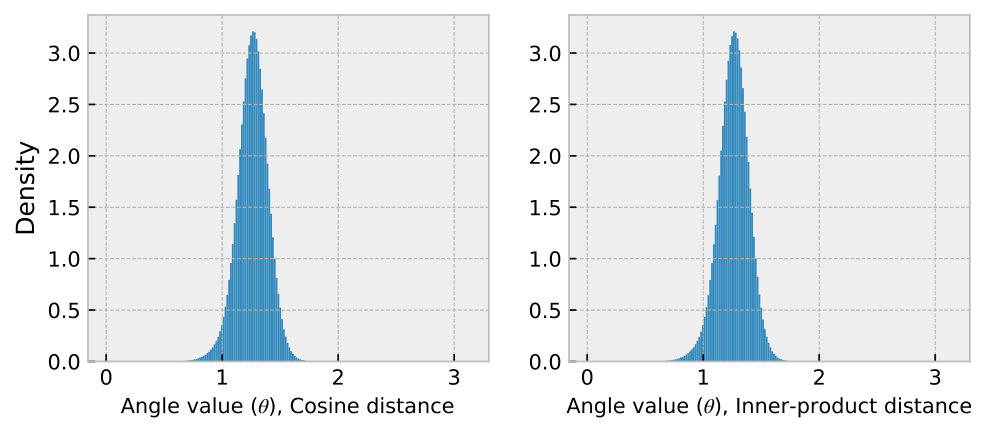 Figure 1
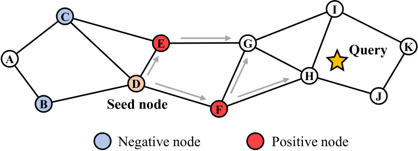 Figure 2
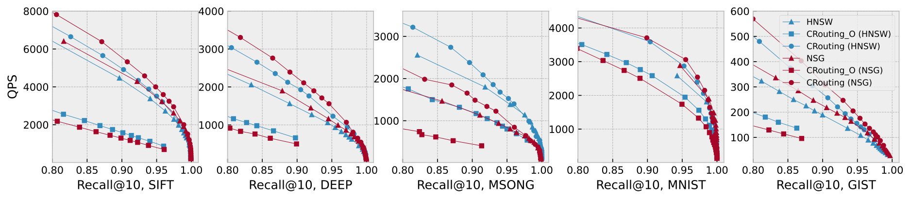 Figure 3
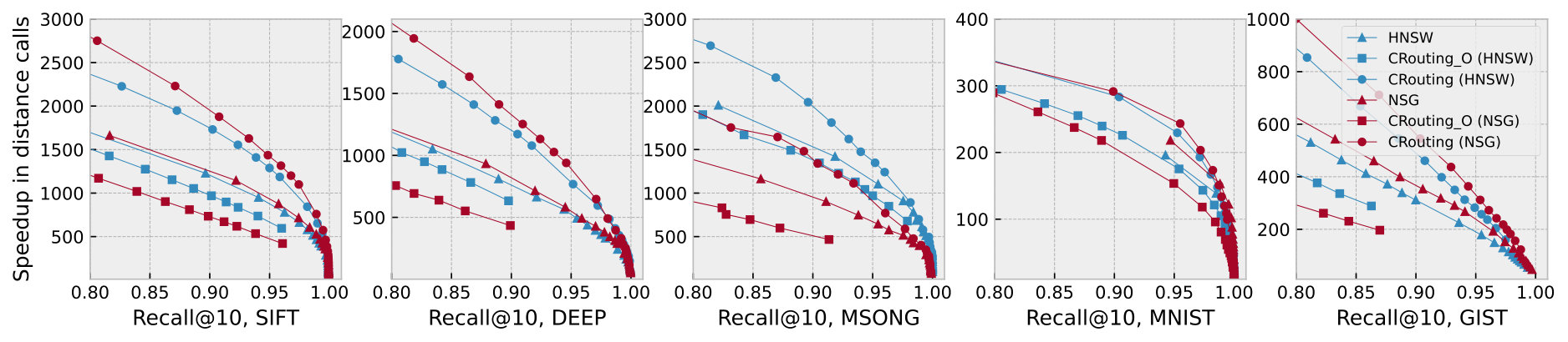 Figure 4
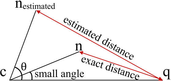 Figure 5
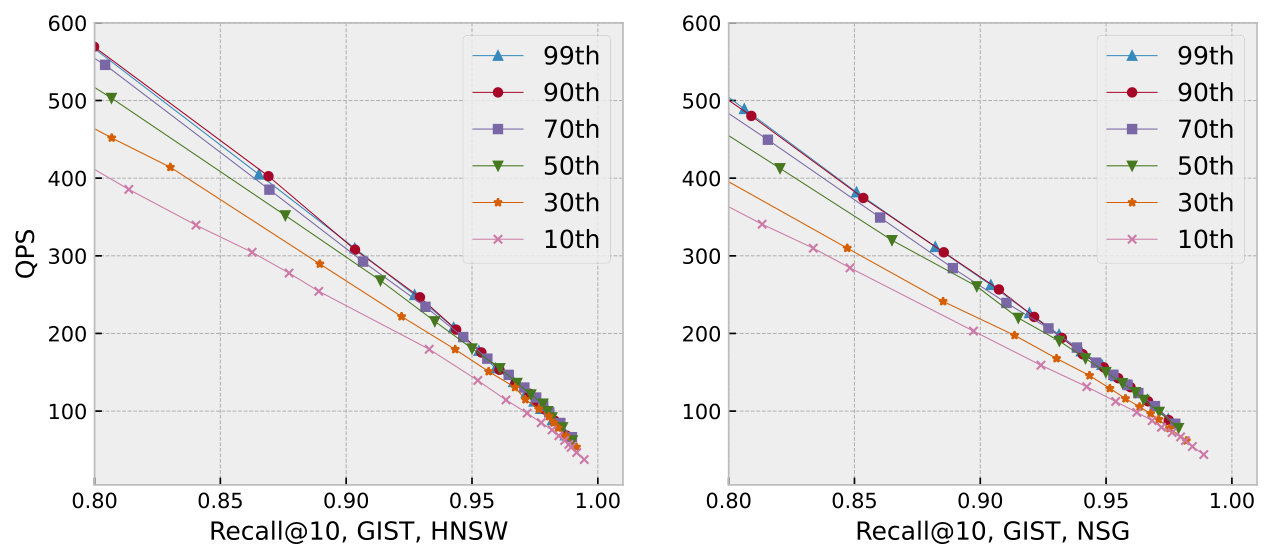 Figure 6
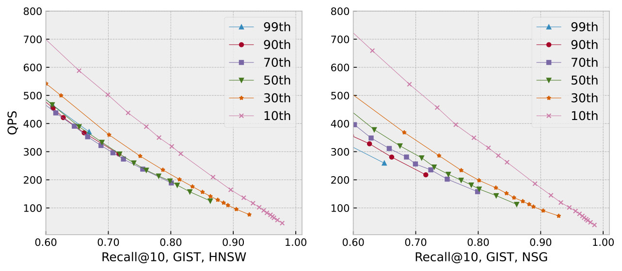 Figure 7
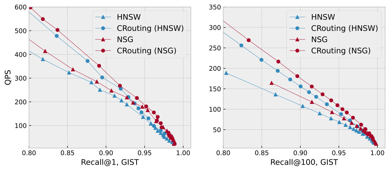 Figure 8
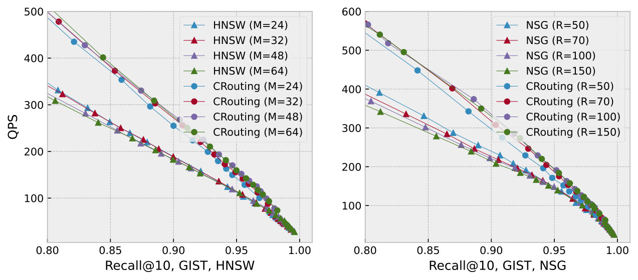 Figure 9
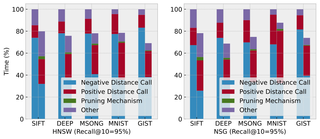 Figure 10
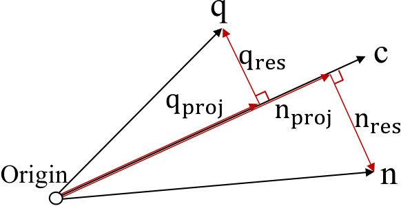 Figure 11
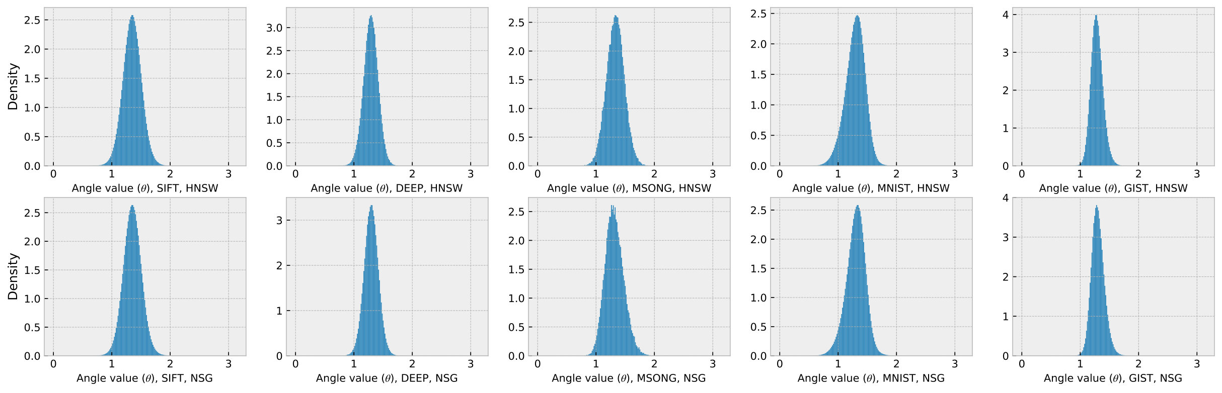 Figure 12
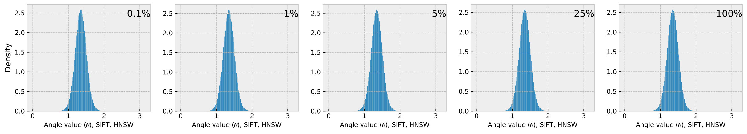 Figure 13
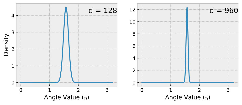 Figure 14
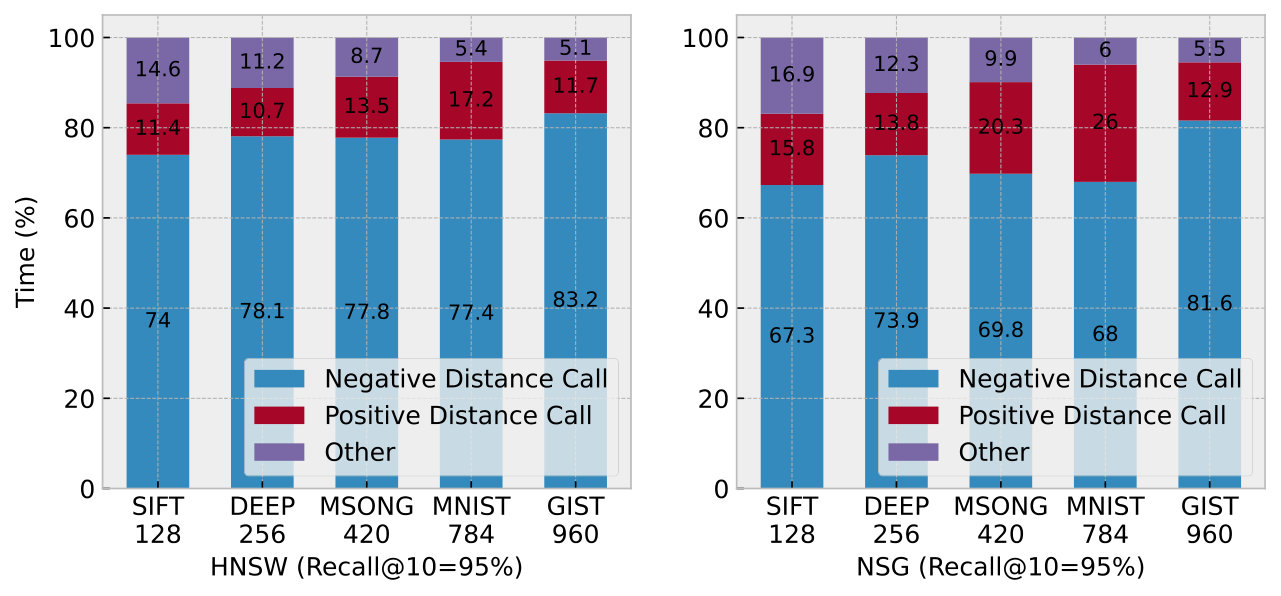 Figure 15
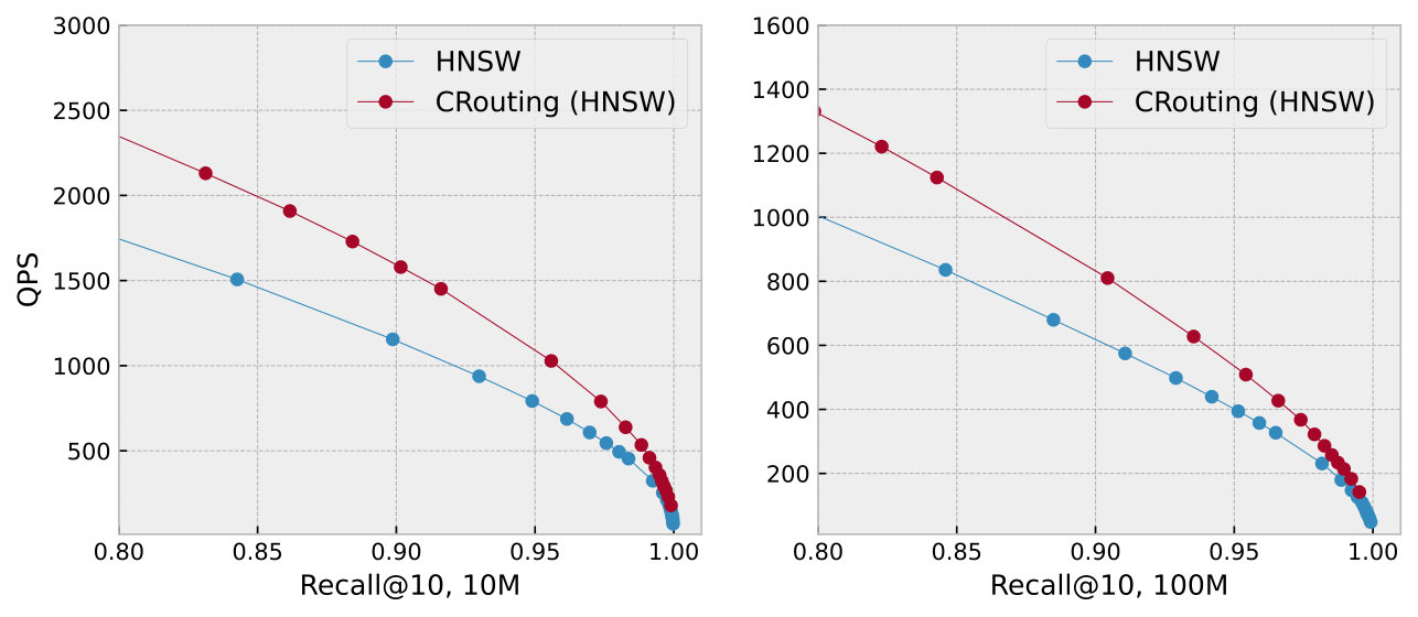 Figure 16
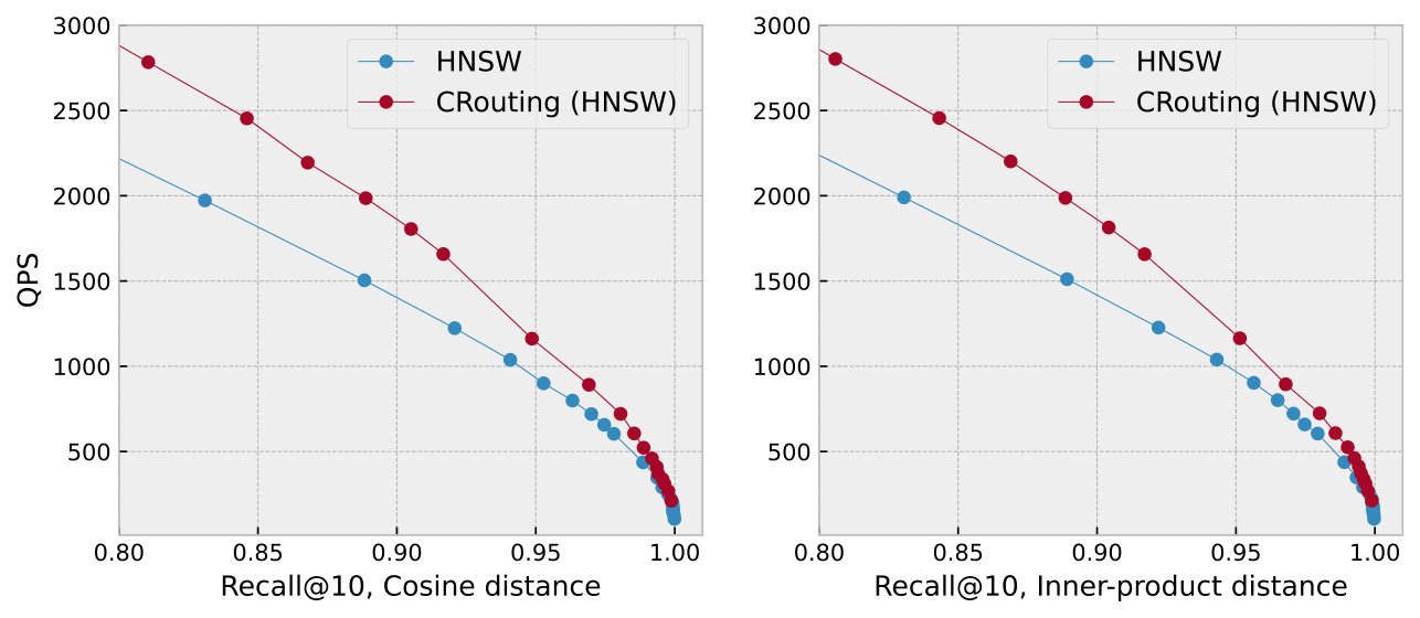 Figure 17
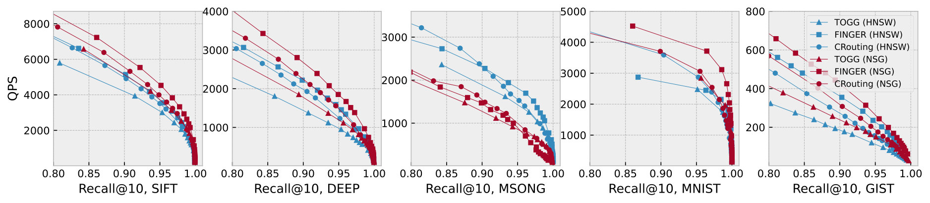 Figure 18
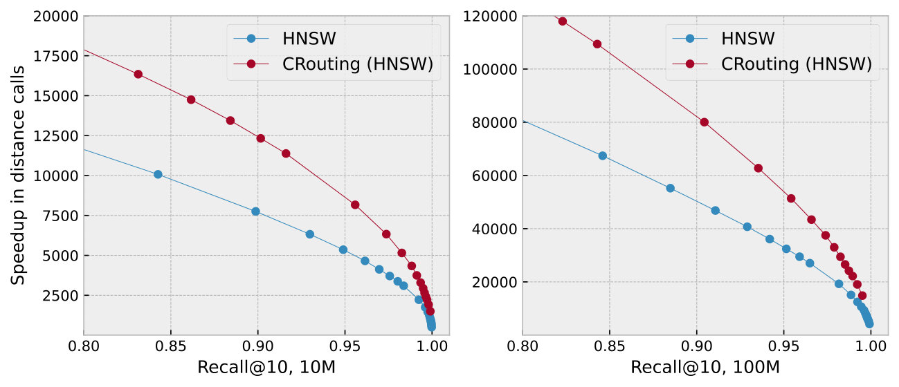 Figure 19
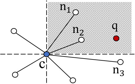 Figure 20
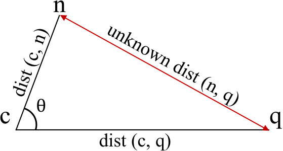 Figure 21
| Strategy | Construction time | Memory footprint | Accuracy |
| TOGG | Fast ✓ | Low ✓ | Low ✗ |
| FINGER | Slow ✗ | High ✗ | High ✓ |
| CRouting | Fast ✓ | Low ✓ | High ✓ |
| efs | HNSW | CRouting_O | CRouting | |||
| Recall | Hop | Recall | Hop | Recall | Hop | |
| 30 | \cellcolorblue!200.889 | \cellcolorblue!201234651 | 0.204 | 233588 | 0.676 | 413111 |
| 40 | 0.921 | 1507433 | 0.256 | 253973 | 0.753 | 489692 |
| 60 | 0.954 | 2032356 | 0.340 | 291073 | 0.842 | 635833 |
| 80 | 0.970 | 2534864 | 0.407 | 325629 | \cellcolorblue!200.886 | \cellcolorblue!20779403 |
| \rowcolorred!20 100 | 0.978 | 3013367 | 0.453 | 358959 | 0.917 | 926499 |
| 200 | 0.994 | 5194785 | 0.620 | 518164 | 0.972 | 1678470 |
| 300 | 0.997 | 7143884 | 0.708 | 672941 | 0.986 | 2431958 |
| 400 | 0.998 | 8934851 | 0.772 | 825041 | 0.992 | 3174724 |
| 500 | 0.999 | 10624804 | 0.808 | 977380 | 0.995 | 3909369 |
| 700 | 0.999 | 13772090 | 0.866 | 1279024 | 0.998 | 5343785 |
| 900 | 0.999 | 16686444 | \cellcolorblue!200.897 | \cellcolorblue!201578669 | 0.998 | 6736528 |
| SIFT | DEEP | MSONG | MNIST | GIST | |
| HNSW | 7.00% | 6.25% | 6.71% | 6.82% | 5.14% |
| NSG | 6.84% | 5.54% | 6.47% | 6.93% | 5.07% |
| SIFT | DEEP | MSONG | MNIST | GIST | |
| HNSW | 3.91% | 4.16% | 3.46% | 2.44% | 5.83% |
| NSG | 3.46% | 3.24% | 4.70% | 2.48% | 5.37% |
| Dataset | HNSW | +TOGG | +FINGER | +CRouting |
| SIFT | 677.1 | 707.8 (+5%) | 771.7 (+14%) | 685.9 (+1%) |
| DEEP | 1163.1 | 1241.7 (+7%) | 1397.1 (+20%) | 1168.1 (+1%) |
| MSONG | 1441.9 | 1508.6 (+5%) | 1702.6 (+18%) | 1461.8 (+1%) |
| MNIST | 46.1 | 49.2 (+7%) | 81.6 (+78%) | 46.5(+1%) |
| GIST | 2881.8 | 3014.7 (+5%) | 3614.9 (+25%) | 2903.3 (+1%) |
| Dataset | NSG | +TOGG | +FINGER | +CRouting |
| SIFT | 163.1 | 193.6 (+19%) | 249.4 (+53%) | 169.1 (+4%) |
| DEEP | 265.2 | 350.8 (+32%) | 474.5 (+79%) | 272.3 (+3%) |
| MSONG | 317.8 | 389.9 (+23%) | 589.6 (+86%) | 325.7 (+2%) |
| MNIST | 13.8 | 16.6 (+20%) | 45.1 (+226%) | 14.3 (+4%) |
| GIST | 806.9 | 960.4 (+19%) | 1546.3 (+92%) | 814.4 (+1%) |
| Dataset | HNSW | +TOGG | +FINGER | +CRouting |
| SIFT | 751.8 | 767.1 (+2%) | 2968.2 (+295%) | 873.8 (+16%) |
| DEEP | 1240.1 | 1255.4 (+1%) | 3456.5 (+178%) | 1362.1 (+10%) |
| MSONG | 1851.3 | 1866.4 (+1%) | 4050.5 (+119%) | 1972.4 (+7%) |
| MNIST | 195.2 | 196.2 (+1%) | 328.3 (+68%) | 202.5 (+4%) |
| GIST | 3925.6 | 3940.9 (+1%) | 6142.1 (+56%) | 4047.7 (+3%) |
| Dataset | NSG | +TOGG | +FINGER | +CRouting |
| SIFT | 620.8 | 636.2 (+3%) | 3264.5 (+426%) | 745.8 (+21%) |
| DEEP | 1142.1 | 1157.3 (+1%) | 3785.7 (+232%) | 1299.8 (+14%) |
| MSONG | 1688.2 | 1703.3 (+1%) | 4311.4 (+156%) | 1778.9 (+5%) |
| MNIST | 184.4 | 185.3 (+1%) | 343.1 (+86%) | 188.7 (+3%) |
| GIST | 3747.4 | 3762.7 (+1%) | 6818.4 (+82%) | 3825.1 (+2%) |
Peer Reviews
No public reviews on file for this paper yet. If you reviewed it on a platform where reviews are public (OpenReview, ICLR, NeurIPS, ICML), you can paste yours below so the community can read it here.
Videos
No videos yet. Explain this paper in a talk, walkthrough, or lecture? Add one.
Taxonomy
TopicsData Management and Algorithms · Advanced Image and Video Retrieval Techniques · Graph Theory and Algorithms
CRouting: Reducing Expensive Distance Calls in Graph-Based Approximate Nearest Neighbor Search
Zhenxin Li
Zhejiang UniversityHangzhouChina
,
Shuibing He
Zhejiang UniversityHangzhouChina
,
Jiahao Guo
Zhejiang UniversityHangzhouChina
,
Xuechen Zhang
Washington State UniversityVancouverUnited States of America
,
Xian-He Sun
Illinois Institute of TechnologyChicagoUnited States of America
and
Gang Chen
0000-0002-7483-0045 Zhejiang UniversityHangzhouChina
Abstract.
Approximate nearest neighbor search (ANNS) is a crucial problem in information retrieval and AI applications. Recently, there has been a surge of interest in graph-based ANNS algorithms due to their superior efficiency and accuracy. However, the repeated computation of distances in high-dimensional spaces constitutes the primary time cost of graph-based methods. To accelerate the search, we propose a novel routing strategy named CRouting, which bypasses unnecessary distance computations by exploiting the angle distributions of high-dimensional vectors. CRouting is designed as a plugin to optimize existing graph-based search with minimal code modifications. Our experiments show that CRouting reduces the number of distance computations by up to 41.5% and boosts queries per second by up to 1.48 on two predominant graph indexes, HNSW and NSG. Code is publicly available at https://github.com/ISCS-ZJU/CRouting.
1. Introduction
Approximate nearest neighbor search (ANNS) finds wide application in areas such as information retrieval (Zhu et al., 2019; Flickner et al., 1995), image and video analysis (Babenko and Lempitsky, 2014b), key-value storage (Shen et al., 2025), and recommender systems (Sarwar et al., 2001), where quick retrieval for the most similar items is crucial (known as the top-K problem). In particular, driven by recent advancements in large language models (LLMs), ANNS services have become a core component of modern AI infrastructure (Lewis et al., 2020). Domain knowledge from various data formats (e.g., documents, images, and speech) is embedded and stored as high-dimensional feature vectors. When a user queries a chatbot, the ANNS engine retrieves semantically similar vectors, delivering relevant contexts to enhance the response quality of LLMs.
The retrieval of exact nearest neighbors in high-dimensional spaces is computationally expensive due to the curse of dimensionality (Indyk and Motwani, 1998). To address this, ANNS offers a practical trade-off by returning an approximate set of the nearest neighbors within an acceptable error margin, thereby achieving efficient scalability for high-dimensional data. Based on the index structure, the existing ANNS algorithms can be divided into four major categories, including tree-structure based approaches (Bentley, 1975; Beygelzimer et al., 2006; Ciaccia et al., 1997; Dasgupta and Freund, 2008), hashing-based approaches (Datar et al., 2004; Gan et al., 2012; Li et al., 2018b; Lu et al., 2020), quantization-based approaches (Babenko and Lempitsky, 2014a, b; Ge et al., 2013b; Gong et al., 2012), and graph-based approaches (Fu et al., 2021, 2019; Malkov et al., 2014; Malkov and Yashunin, 2018). Among these, graph-based algorithms, such as HNSW (Malkov and Yashunin, 2018) and NSG (Fu et al., 2019), have shown promising search performance over other approaches (Wang et al., 2021a; Li et al., 2019). They efficiently explore neighborhood structures by constructing a graph where nodes represent feature vectors and edges denote potential nearest neighbor relationships. Graph-based methods scale effectively with large datasets and adapt well to various data distributions. As a result, they form the foundation of various ANNS services and vector databases, including ElasticSearch (Grand, 2023), FAISS (Johnson et al., 2019), Milvus (Wang et al., 2021b), VSAG (Zhong et al., 2025), and PostgreSQL (Yang et al., 2020).
The graph-based ANNS algorithms commonly use the greedy search algorithm for searching nearest neighbors. As shown in Figure 1, it maintains a candidate set where candidates are assessed based on their distance from the query point. Starting from the specified seed node, each candidate’s neighbors are examined. Neighbors whose distances to the query exceed the farthest distance in the candidate set are discarded (i.e., negative nodes), while others are included in the candidate set and further refined (i.e., positive nodes). The iterative distance calculation calls find nodes closer to the query, progressively moving towards the query point.
However, repeated distance calculations in high-dimensional spaces are costly and constitute the primary time bottleneck in ANNS. For example, our experiments show that distance calculations account for at least 83% of the total running time across five widely used datasets with varying sizes and dimensionalities (§ 2.2). Furthermore, the majority of nodes involved in these calculations are negative objects, meaning they will not be included in the candidate set and do not affect the final result. Based on these observations, it suggests that developing a method to prune negative nodes could reduce expensive distance calculations without compromising accuracy.
Various routing techniques are proposed to improve the performance of graph-based ANNS. The primary objective is to minimize distance computations during neighbor exploration. For example, HCNNG (Munoz et al., 2019) and TOGG (Xu et al., 2021) employ KD-trees (Bentley, 1975) to select points in the same direction as the query thereby only exploring a subset of neighbors for each search iteration. However, they tend to yield suboptimal query accuracy because of incorrect pruning, limiting their effectiveness. FINGER (Chen et al., 2023) pre-computes and stores the residual vectors for all nodes’ neighbors during construction, allowing for rapid distance estimation and node pruning during search. Other ML-based optimizations (Baranchuk et al., 2019; Prokhorenkova and Shekhovtsov, 2020; Li et al., 2020) learn routing functions, utilizing additional representations to facilitate optimal routing from the starting node to the nearest neighbor. However, all these optimizations either compromise search accuracy or necessitate additional training and extra information, leading to increased construction time and memory footprint.
In this paper, we propose CRouting, a novel routing strategy to guide the navigation for graph-based ANNS. Compared to existing routing strategies, CRouting achieves a favorable balance between search and construction efficiency. CRouting take inspiration from the characteristics of high-dimensional vector distribution: in high-dimensional spaces, two random vectors are almost always very close to orthogonal (Ball et al., 1997). Following this theorem, in the triangles formed by the current search node, the query node, and the neighboring node, we observe that the angles associated with the current search node tend to concentrate around a specific value. Based on this observation, CRouting uses the cosine theorem to efficiently estimate the distance between the neighbor node and the query node. The estimated distance is used to decide whether to prune the neighbor, thereby reducing unnecessary computational overhead. Since the estimated distance may have approximation errors, some nodes might be incorrectly pruned. CRouting further introduces a technique to identify these incorrectly pruned nodes and recalculate their exact distances to the query to ensure high accuracy. In summary, this paper makes the following contributions:
- •
We conduct a thorough analysis of existing graph-based ANNS algorithms and find that all of them are plagued by repeated distance computations, which account for the majority of the overall search operation costs.
- •
We propose CRouting, a novel routing strategy that guides navigation by leveraging the characteristics of high-dimensional vector distributions. Collaborated with an error-correction technique, CRouting effectively prunes massive unnecessary distance computations under the same accuracy criteria.
- •
We implement CRouting and develop it as a plugin to enhance HNSW and NSG, two predominant graph-based ANNS algorithms. Our evaluation results show that CRouting reduces the number of distance computations by up to 41.5% while maintaining the same accuracy, thereby improving queries per second (QPS) by up to 1.48.
2. Background and Motivation
2.1. Greedy Search
The greedy search algorithm is commonly used in most graph-based methods for finding nearest neighbors. As shown in Algorithm 1, given a query point and a starting point , the algorithm is designed to search for nearest neighbors to . It maintains two priority queues: candidate queue that stores potential candidates to expand and top results queue that stores the current most similar candidates. At each search iteration, it first extracts the current nearest point in and gets the furthest distance to the query from as an (lines 3-4). And then it visits ’s neighbors and computes their distance to respectively to expand the candidates. For each neighbor, it checks whether its distance from is less than the and if so, it pushes the neighbor into both and , and updates the simultaneously (lines 11-14). The repeated distance calls constitute the primary time cost (line 11).
2.2. Running Time Analysis
We measure the time consumption of greedy search across five public datasets using two state-of-the-art graph-based ANNS algorithms: HNSW and NSG. In this test, if a node is added to the candidate queue after triggering a distance calculation, we refer to it as a positive node; otherwise, it is termed a negative node.
As shown in Figure 2, when the data dimensionality increases from 128 to 960, the proportion of time spent on distance calculations rises from 85.4% to 94.9% on the HNSW algorithm, and from 83.1% to 94.5% on the NSG algorithm, respectively. Moreover, we observe that the majority of nodes are negative, indicating that these nodes will not be added to the candidate set and will not have any further impact on the final result. This suggests that if we can develop a method to prune these negative nodes, we could significantly reduce expensive distance calculations without compromising accuracy.
2.3. Existing Routing Strategies
Several routing techniques have been proposed to minimize distance computations during neighbor exploration. Here, we describe two state-of-the-art routing strategies, including TOGG and FINGER, which we use in the experimental section for comparison with CRouting.
TOGG introduces a two-stage routing strategy that combines optimized guided search with a greedy algorithm. The routing process is explicitly divided into two detailed stages: (S1) the routing stage that is farther from the query and (S2) the routing stage that is closer to the query. In stage S1, the primary focus is on quickly identifying the neighborhood of the query to enable prompt routing toward it. To achieve this, TOGG utilizes KD-trees to select points aligned with the query direction, thereby allowing it to explore only a subset of neighbors during each search iteration, as illustrated in Figure 3. In contrast, stage S2 emphasizes the need to thoroughly explore vertices near the query in order to obtain sufficiently accurate search results. Consequently, this stage not only examines the neighbors of each vertex in the candidate set but also investigates the neighbors of those neighbors. By relaxing the expansion constraint compared to traditional greedy algorithms, TOGG effectively mitigates the risk of getting trapped in local optima. However, the utilization of KD-trees for navigation may result in reduced accuracy, as numerous potential nodes are filtered out during stage S1 and cannot be reintegrated in stage S2.
FINGER estimates the distance between each neighbor and the query. Specifically, for each node, it generates projected vectors locally for both neighbors and the query to define a subspace, and then applies Locality Sensitive Hashing (LSH) (Charikar, 2002) to approximate the residual angles. As illustrated in Figure 4, the distance is decomposed as follows:
[TABLE]
During graph construction, FINGER will calculate and store (1 byte), (4 bytes), projection coefficient (, 4 bytes), and other relevant LSH information for estimating the angle between and . Then, FINGER can quickly estimate distances and eliminate unnecessary calculations during query processing. However, this method necessitates additional computation and supplementary information, leading to increased time and memory overhead for graph construction.
Existing routing strategies either compromise search accuracy or require additional construction overhead. In contrast, CRouting strikes a favorable balance between search and construction efficiency. Table 1 compares CRouting with existing routing strategies, and the detailed experimental results are presented in § 5.7.
3. Problem Definition and Analysis
In this section, we present the insight behind CRouting, an effective distance estimation method that leverages the characteristics of high-dimensional vector distributions.
3.1. Problem Statement
As shown in Figure 5, during each search iteration, given a query , a current search node , and a specific neighbor of called , traditional greedy search algorithms compute the exact Euclidean distance between and (i.e., ), with a time complexity of , where is the data dimension. Our objective is to approximate this distance. If the estimated distance exceeds the (i.e., the furthest distance to the query from the top results queue as stated in Algorithm 1), then node can be pruned. This approach ensures that only nodes with a potential to be closer to the query are considered, thus optimizing the search process and reducing computational overhead.
3.2. Naive Solution: Triangle Inequality
Currently, we only know because is extracted from the candidate queue, and is pre-calculated in a previous search iteration. However, this information alone is insufficient to estimate . Note that is a neighbor of , so was calculated during the graph construction and can be retained in memory.
After obtaining the exact lengths of the edges (i.e., and ), we can directly apply the triangle inequality to estimate the lower bound of the third edge’s length. Specifically, in :
[TABLE]
And if is greater than the , we can directly prune node . However, our research shows that this method is not always effective. For instance, it reduces the number of distance computations by only 0.08% using the SIFT dataset on the HNSW algorithm, which is negligible in the overall search process. Although the triangle inequality provides an accurate lower bound, it is often too loose to effectively filter out nodes.
3.3. Optimized Solution: Cosine Theorem
To obtain a more accurate distance estimation, additional information, the angle ( in Figure 5), is required. With this angle, we can then calculate using the cosine theorem.
The distribution of vectors in high-dimensional spaces has a unique property: in high-dimensional spaces, two random vectors are almost always very close to orthogonal. The probability density function of the angle between two randomly selected vectors can be formulated as follows:
[TABLE]
where is the dimensionality of the vector and is the Gamma function. This indicates that the angle distribution is solely determined by the dimensionality of the vectors. To better understand, Figure 6 plots the probability density for and . As increases, the values of become increasingly concentrated around (orthogonal).
Inspired by this, we question whether the angle between vectors and in Figure 5 satisfies the above equation. Because the position of neighbor is completely random with respect to the current node , the direction of vector relative to is independent. Therefore, the values of angle may also exhibit special distribution characteristics.
To further verify this, we record the values of along the search paths across different datasets and algorithms using randomly generated queries. The number of queries varies from 0.1% to 100% of the number of nodes to construct the graph. From the results in Figure 7 and Figure 8, we have the following observations. (1) We observe that the values of follow a skewed distribution, with the center around , which is similar to the trend shown in Figure 6. (2) We observe that the distribution of angles is determined solely by the dataset and remains unaffected by the graph construction algorithm or the number of query nodes. This indicates that the angle distribution is an intrinsic property of the dataset. Because the dataset’s vector dimensionality and distribution remain constant, the angle distribution can be used indefinitely once computed.
Based on these observations, we propose the key design concept of CRouting. For each dataset, CRouting selects a specific angle derived from its angle distribution (i.g., the central point) to set the value of in the cosine theorem. Given that the angle exhibits a skewed characteristic, using a single representative value for all the angle values along the search path enables a efficient estimate of while keeping the distance estimation error within a small range.
4. CRouting Design
This section describes the graph construction and query processes of CRouting. CRouting is designed as a plugin to improve the query performance of existing graph-based ANNS algorithms.
4.1. Graph Construction
Acquisition of additional information. As a prerequisite for CRouting, we need to obtain two additional pieces of information during graph construction: (1) the distances between each node and all its neighbors, and (2) the angle distribution of . The distances between each node and its neighbors are already calculated during the graph construction process in all the existing graph-based ANNS algorithms. CRouting simply saves them in memory rather than discarding them. To obtain the angle distribution, we will randomly generate query nodes after the graph has been constructed. On the search paths of these nodes, we simultaneously use the cosine theorem to calculate the angle values.
Extra time overhead. By default, the value of is set to 0.1% of the number of nodes used to construct the graph. Because the sampling frequency is sufficient to obtain an accurate angle distribution (as shown in Figure 8), while the computational overhead remains negligible. Our experiments show that the additional construction time does not exceed 4% (§ 5.7).
Extra memory overhead. One concern is that storing distances between neighbors incurs extra memory overhead. In graph-based ANNS algorithms, memory is used for storing high-dimensional vectors, graph indexs, and distance values () saved by CRouting. Our study shows that leads to an additional 2% to 21% overhead compared to the approaches without using CRouting (§ 5.7). The ratio of additional memory consumption is decreased as the dimensionality of datasets is increased.
4.2. Graph Search
Pruning strategy. By utilizing the stored and , along with the angle obtained from the distribution of high-dimensional random vectors (§ 3.3), we can efficiently estimate using the cosine theorem. If is not less than the , we can avoid making the expensive distance call to calculate the exact distance. Otherwise, the normal routing process will proceed as usual. Adjusting the angle allows us to control the threshold for the pruning strategy. Specifically, larger angle values lead to more nodes being pruned, but they also increase the estimation error, impacting accuracy. Thus, there is a trade-off between accuracy and the number of distance calculations. We evaluate it in detail in § 5.5.
Error correction. Although many unnecessary nodes can be effectively pruned, a significant issue remains. Our pruning strategy may introduce approximation errors, which may lead to the removal of important nodes and notably impact the final results. For instance, as illustrated in Figure 9, given a query and the current search node , we expand the search by exploring the neighbors of . The specific neighbor node , which lies in the direction of (i.e., with an extremely small angle), is closer to than , making it a strong candidate for refining the final results. However, for such neighbors, the error in our estimated distance compared to the actual distance can be significant, raising the likelihood that these promising nodes are mistakenly pruned. Additionally, the convergence paths from these neighbors may also be overlooked, negatively impacting accuracy.
To address this issue, we devise an error correction mechanism to identify erroneously deleted nodes. The key idea is that nodes mistakenly pruned and located near the query node are likely to be revisited in subsequent searches because of the graph’s connectivity. This means that even if some positive nodes are pruned initially, they can still be reached through alternative paths in later stages of the search. For example, as shown in Figure 1, if node is pruned while evaluating the neighbors of node , it will still be revisited when expanding from node . Based on this idea, if a node has been pruned by CRouting, any future access to that node should involve calculating its exact distance to ensure high accuracy.
Put it all together. Algorithm 2 describes the graph search process of CRouting. Compared to the existing ANNS algorithms using greedy search (e.g., Algorithm 1), CRouting uses the approximated distance to aggressively prune nodes (lines 10-13) before each exact distance calculation (line 15). Errors may happen when a node is marked as “pruned” (line 12). In this case, when the node is revisited in the future search, CRouting will mark the node as “visited” and calculate the exact (lines 14-15). We design CRouting as a plug-in that can be applied on top of any existing graph-based ANNS algorithms that utilize greedy search, requiring only minimal changes to the existing code.
4.3. Applicability to Other Distance Metrics
In addition to Euclidean distance, CRouting can be easily extended to two other commonly used distance metrics: inner-product and cosine distance, through simple transformations. For a query and data point with an angle between them, the inner-product distance is given by: . The relationship between Euclidean and inner product distance is:
[TABLE]
Since the calculation of is a one-time operation for each query, it remains computationally inexpensive. Moreover, (i.e., the norm for each inserted vector) can be precomputed and stored during the graph construction phase. The associated space and time costs are acceptable. Specifically, the space required for storing the norm of a vector (typically with dimensions greater than 100) is less than 1%. The computational cost of calculating the norm one time is negligible compared to the numerous distance calculations required for graph construction. In addition, the cosine distance is equivalent to the inner-product distance on normalized data and query vectors (Gao and Long, 2023), where CRouting is still applicable. We evaluate the generality of CRouting in § 5.6.
5. Evaluation
Our experiments involve three folds. First, we compare our methods with traditional graph-based approaches to empirically demonstrate that CRouting can be integrated into graph-based greedy search methods for improved performance. Second, we evaluate the sensitivity, generality, and scalability of CRouting in various scenarios. Third, we compare our methods with other routing strategies to assess their efficiency and effectiveness.
5.1. Experimental Setting
Implementation setup. We run the experiments on a Linux server with two Intel Xeon Gold 5318Y CPUs. Each CPU has 24 physical/48 logical cores, DRAM. All source codes are compiled with g++10.3 with -O3 optimization. Following previous work (Gao and Long, 2023; Wang et al., 2021a; Li et al., 2019), we disable all hardware-specific optimizations such as SIMD and memory prefetching so as to focus on the comparison among algorithms themselves. To improve construction efficiency, the code involving vector calculation is parallelized for the index construction. All tests are evaluated on a single thread by default.
Datasets and metrics. We use five public datasets with varying sizes and dimensionalities, detailed in Table 2. They are commonly employed to benchmark ANNS algorithms (Aumüller et al., 2020). We use the Euclidean distance as the distance metric by default. The comparison metrics used to evaluate performance are: (1) Recall@K: it measures search accuracy by comparing the approximate point set found for a given query with the true nearest neighbor result set . It is defined as: . By default, is set to 10. (2) QPS: it indicates the number of queries a machine can handle per second. (3) Speedup in distance calls (Xu et al., 2021; Chen et al., 2023; Wang et al., 2024): it measures the efficiency of a method by comparing the number of distance calculations. It is defined as the ratio of distance calculations in the brute-force method to those in the optimized routing method. Since the accuracy and performance of greedy search can vary on the size of the candidate array (see Algorithm 1), we adjust to plot both the recall–QPS curve and the recall–speedup curve.
Target comparisons. We implement CRouting on HNSW111https://github.com/nmslib/hnswlib and NSG222https://github.com/ZJULearning/nsg, two widely used graph indexes for ANNS in production services like Facebook AI Research (Johnson et al., 2019) and Alibaba e-commerce search (Fu et al., 2019). We follow the default parameter settings of their public code. For HNSW, the neighbor limit for each vector is set to 32 and the insertion candidate neighbor limit is set to 256. For NSG, the neighbor limit is set to 70, the insertion candidate neighbor limit is set to 500, and the insertion priority queue length is set to 60. We first compare CRouting with initial HNSW and NSG algorithms to demonstrate how CRouting accelerates them. Then, we compare CRouting with two currently leading-edge routing strategies including (1) TOGG333https://github.com/whenever5225/TOGG, which uses KD-trees to select querying neighbor nodes, and add a fine-tuned step when searching nodes near the query and (2) FINGER444https://github.com/Patrick-H-Chen/FINGER/tree/main, which approximates the distance function in graph-based methods by estimating angles between neighboring residual vectors. Moreover, we evaluate two variants of our systems to distinguish the effect of each proposed design component. Specifically, CRouting_O refers to the version that only enables the pruning strategy while CRouting incorporates both pruning and error-correction strategies.
5.2. Improvements over ANNS Algorithms
Figure 10 plots the recall-QPS curves on five datasets. We focus only on the region with the recall at least 80% based on practical needs. Overall, we can observe clearly that CRouting exhibits the best performance across all datasets. CRouting improves the QPS of HNSW and NSG by 1.12 to 1.48 and 1.11 to 1.47, respectively. This demonstrates the effectiveness of our methods. We also find that the performance of CRouting_O is significantly poor, even falling below the original algorithms. This indicates that relying solely on the pruning strategy is insufficient, as it results in the incorrect deletion of a large number of nodes.
To further analyze the reasons behind the performance improvement, we show the detailed recall-speedup curves in Figure 11. The recall-speedup curves display a trend similar to the recall-QPS curves. CRouting achieves a speedup in distance calls ranging from 1.22 to 1.58 compared to HNSW, and from 1.15 to 1.71 compared to NSG, indicating a significant reduction in the number of distance calculations, thereby enhancing the QPS.
Moreover, we decompose the time cost when targeting 95% recall in Figure 12. We observe that CRouting reduces the distance calculation time for negative nodes by 47.4% to 61.6%, supporting our motivation discussed in § 2.2. While CRouting introduces additional checks for the pruning mechanism, it still reduces the overall running time by 12.4% to 31.4%. The pruning mechanism accounts for only 0.7% to 3.9% of the total time. This low overhead is primarily due to the fact that a single cosine calculation involves only a few multiplications and additions. In contrast, calculating the exact distance for a -dimensional vector requires multiplications, additions, and a single random memory read operation. Thus, the pruning algorithm results in significant performance gains.
5.3. Ablation Study
The accuracy and performance of the greedy search can vary depending on the size of the candidate array (see Algorithm 1). Table 3 illustrates the recall@10 and hop (i.e., the number of distance calls) for different values of . When equals 100 (highlighted in pink), CRouting_O reduces the number of hops by 90% of the original greedy search algorithm, but at the cost of a significant drop in recall (from 97% to 45%). In contrast, enabling the error-correction technique allows CRouting to achieve 91% recall. Although this results in more hops than CRouting_O, CRouting still reduces the number of hops by 70% compared to the original greedy search.
The pruning strategy sacrifices accuracy for performance, ensuring a substantial reduction in the number of distance calls. On the other hand, the error-correction strategy sacrifices performance for improved accuracy. Because the revisited nodes have a higher likelihood of being positive nodes, it is worthwhile to recalculate their distances. By combining both techniques, CRouting achieves a better balance between performance and accuracy. For instance, when recall reaches around 89% (highlighted in purple), CRouting reduces the number of hops by 36.9% compared to the original greedy search, and by 50.6% compared to CRouting_O.
5.4. Error Analysis
Although we cannot mathematically prove the approximation error bounds of CRouting, we assess two accuracy metrics: relative error and the incorrect pruning ratio, to empirically verify that its accuracy is acceptable. Table 4 presents the relative error between the estimated distance and the true distance . The relative error is defined as . The average relative error of CRouting is approximately 6%. Additionally, Table 5 displays the number of false negatives, where nodes incorrectly classified as negative are actually positive. The maximum ratio of incorrect pruning remains below 6% across all datasets. These results demonstrates the effectiveness of CRouting in distance estimation.
5.5. Sensitive Analysis
The only parameter introduced by CRouting is the pruning threshold (i.e., the value of ). Other parameters, such as the number of neighbors, and , and result number , are inherent to the graph-based ANNS algorithms and are set based on dataset dimensions, accuracy requirements, and latency constraints.
Effect of the pruning threshold. Figure 13 illustrates the impact of varying the pruning threshold by adjusting the angle from the 10th to the 99th percentile of the angle distribution. Larger angles for CRouting_O generally result in lower performance. In contrast, for CRouting with error-correction technique enabled, selecting a larger angle typically leads to improved performance. This is because larger angles aggressively prune more nodes, which enhances the QPS. Although this increases the likelihood of mistakenly pruning some nodes, the accuracy loss from such errors can be mitigated by our error-correction mechanism. Across all datasets and algorithms, we consistently observe the best performance at the 90th percentile. Consequently, we set the pruning threshold to the angle value at 90th percentile.
Effect of the number of neighbors. The parameters and control the number of connected neighbors on HNSW and NSG algorithms, respectively, and this number directly influences the overall size of the graph. In practical applications, users often adjust the number of neighbors based on their memory capacity and recall requirements. Figure 14 shows the recall-QPS curves of CRouting on the GIST dataset with varying numbers of neighbors. CRouting consistently enhances QPS in all scenarios. Additionally, we find that as the number of neighbors increases, the performance improvements brought by CRouting become more pronounced. As the dimensionality of real-world data increases, more complex and intricate graphs are needed to achieve high recall (Malkov and Yashunin, 2018; Fu et al., 2019). This inevitably increases the number of connected neighbors, making our approach more attractive.
Effect of the result number. The parameter in Recall@K represents the result number. Figure 15 shows the recall-QPS curves for and on the GIST dataset. As increases, the routing becomes more challenging, yet CRouting consistently accelerates the search by at least 30% when targeting 80% recall, demonstrating its robustness across different .
5.6. Generality and Scalability
Other distance metrics. We assess the generality of CRouting for cosine and inner-product distance metrics. Figure 16(a) shows that the angle distributions with other metrics are similar to that of the Euclidean distance. Using other distance metrics does not change the directional randomness between a node and its neighbors, and the angular distribution still exhibits a skewed characteristic. Therefore, the pruning strategy of CRouting remains effective. As shown in Figure 16(b), CRouting achieves consistent improvements in QPS across different distance metrics.
Search on large datasets. We evaluate the scalability of CRouting in terms of data volume by sampling 10 million and 100 million vectors from the SIFT-1B dataset (Anon, 2010). The SIFT-100M dataset represents the largest dataset that can be processed on our machine. Figure 17 shows the recall-speedup and recall-QPS curves. The results demonstrate that CRouting consistently outperforms the baseline algorithms across all data volumes.
5.7. Comparison to Previous Routing Strategies
Figure 18 illustrates the recall-QPS curves for various routing strategies, with all competitors employing consistent index parameters. Across all datasets, TOGG exhibits the poorest performance. This is primarily due to the use of the KD-tree for filtering out neighbors that differ in direction from the query node, which is often inaccurate in high-dimensional spaces, as confirmed by previous research (Wang et al., 2021a). Both CRouting and FINGER achieve higher QPS than TOGG. Although FINGER’s QPS is approximately 10% higher than CRouting, it requires more construction time and incurs higher space costs for graph construction.
From the results presented in Table 6, we observe that the construction time of CRouting increases by no more than 1% on the HNSW algorithm and by no more than 4% on the NSG algorithm. Conversely, the construction time of FINGER increases by 14% to 78% on the HNSW algorithm, and increases by 53% to 226% on the NSG algorithm. FINGER requires more indexing time due to the need to construct an additional subspace for each node. This also explains why it has a higher QPS, as a substantial portion of the computational tasks during the search phase are offloaded to the construction process. Table 7 shows the results of index size. The memory footprint of CRouting increases by 2% to 21% due to the requirement to store the distances to neighboring nodes. FINGER incurs pronounced space costs to store the information about projected vectors and LSH. Specifically, the memory overhead of FINGER increases by 56% to 295% on the HNSW algorithm and by 82% to 426% on the NSG algorithm.
Construction time and space are critical performance metrics in vector databases. Indexes for vector search are typically rebuilt weekly (Li et al., 2018a) to balance low query latency, high accuracy, and the daily updates of billions of vectors. However, the process of graph reconstruction incurs significant resource overhead. For instance, building a global graph-based index for a 128 GB, 128-dimensional SIFT dataset with 1 billion vectors requires 1100 GB of memory over 2 days, or 5 days with 64 GB of memory and 32 vCPUs (Subramanya et al., 2019). FINGER significantly increases both construction time and index size, making it particularly costly in such scenarios. CRouting exhibits strong competitiveness in both construction and query efficiency for graph-based ANNS algorithms, making it a compelling choice for routing strategies.
6. Related Work
Approximate Nearest Neighbor Search (ANNS). Existing ANNS algorithms can be categorized into four main types: (1) graph-based methods (Fu et al., 2021, 2019; Malkov et al., 2014; Malkov and Yashunin, 2018; Subramanya et al., 2019; Munoz et al., 2019; Li et al., 2019; Harwood and Drummond, 2016), (2) quantization-based methods (Gao and Long, 2024; Babenko and Lempitsky, 2014a, b; Ge et al., 2013b; Gong et al., 2012; Guo et al., 2020; Jegou et al., 2010; Ge et al., 2013a), (3) tree-based methods (Beygelzimer et al., 2006; Ciaccia et al., 1997; Dasgupta and Freund, 2008; Muja and Lowe, 2014; Ram and Sinha, 2019; Arora et al., 2018; Silpa-Anan and Hartley, 2008; Curtin et al., 2013), and (4) hashing-based methods (Datar et al., 2004; Gan et al., 2012; Li et al., 2018b; Lu et al., 2020; Sun et al., 2014; Tao et al., 2010; Zheng et al., 2020; Gong et al., 2020; Huang et al., 2015). Notably, graph-based approaches demonstrate superior performance for in-memory ANNS. In contrast, quantization-based methods excel in scenarios with limited memory resources. Additionally, a substantial body of research has explored the application of machine learning techniques to accelerate searches (Dong et al., 2020; Feng et al., 2023; Baranchuk et al., 2019; Prokhorenkova and Shekhovtsov, 2020; Li et al., 2020). For further details, we direct readers to recent tutorials (Echihabi et al., 2021; Qin et al., 2021; Tian et al., 2023), as well as comprehensive reviews and benchmarks (Wang et al., 2021a; Li et al., 2019; Aumüller et al., 2020; Boytsov and Naidan, 2013; Patella and Ciaccia, 2009).
Routing strategies. TOGG (Xu et al., 2021) and HCNNG (Munoz et al., 2019) utilize KD-trees to ascertain the direction of the query, effectively narrowing the search to vectors aligned with that specified direction. FINGER (Chen et al., 2023) leverages Locality Sensitive Hashing to estimate the distance of each neighbor from the query. Additionally, other machine learning-based optimizations (Baranchuk et al., 2019; Prokhorenkova and Shekhovtsov, 2020; Li et al., 2020; Gupta et al., 2022; Li et al., 2024; Antol et al., 2021) develop a routing function that employs supplementary representations to enhance routing efficiency from the starting node to the nearest neighbor. However, all these optimizations either sacrifice search accuracy or require extra computational resources, resulting in prolonged graph construction times. In contrast, CRouting strikes a favorable balance between search and construction efficiency.
Other Optimizations. As the volume of vector data continues to increase, there has been a surge in interest around supporting incremental updates to vector indexes (Xu et al., 2023; Singh et al., 2021; Mohoney et al., 2024), a crucial technique for enabling efficient and accurate for ANNS. Some studies (Wang et al., 2024; Gollapudi et al., 2023) focus on developing efficient and robust frameworks for hybrid query processing, which integrates ANNS with attribute constraints. Additionally, several efforts have optimized ANNS for newer hardware. For example, GPU-based ANN indexes such as SONG (Zhao et al., 2020) and GGNN (Groh et al., 2022) have been proposed, achieving up to two orders of magnitude speedup over CPU-based methods. HM-ANN (Ren et al., 2020) redesigns the HNSW algorithm using Intel Optane persistent memory (Newsroom, 2019). CXL-ANNS (Jang et al., 2023) decouples DRAM from the host via Compute Express Link (Consortium, 2020), placing all essential datasets into its memory pool to handle billion-point graph-based ANNS. FANNS (Jiang et al., 2023) automatically co-designs hardware and algorithms on FPGAs based on user-defined recall requirements and hardware resource budgets. These advanced optimizations are orthogonal to our work and can be incorporated in future research efforts.
7. Conclusions
We propose CRouting, a novel routing strategy designed to enhance navigation in graph-based ANNS algorithms. CRouting approximates the distance function by leveraging the angle distributions of high-dimensional vectors, enabling the avoidance of unnecessary distance calculations. It is designed as a plugin to optimize existing graph-based search with minimal code modifications. Our experiments show that CRouting reduces the number of distance computations by up to 41.5% across two state-of-the-art algorithms, HNSW and NSG, while maintaining the same accuracy, thereby enhancing the overall QPS by up to 1.48.
The reference list from the paper itself. Each links out to its DOI / PubMed record.
- 1(1)
- 2Anon (2010) Anon. 2010. Datasets for approximate nearest neighbor search. http://corpus-texmex.irisa.fr/ . Last accessed on Sep-2024.
- 3Anon (2011) Anon. 2011. Million Song Dataset Benchmarks. http://www.ifs.tuwien.ac.at/mir/msd/ . Last accessed on Sep-2024.
- 4Anon (2018) Anon. 2018. Deep 1M Dataset. https://www.cse.cuhk.edu.hk/systems/hash/gqr/datasets.html . Last accessed on Sep-2024.
- 5Antol et al. (2021) Matej Antol, Jaroslav Ol’ha, Terézia Slanináková, and Vlastislav Dohnal. 2021. Learned metric index—proposition of learned indexing for unstructured data. Information Systems 100 (2021), 101774.
- 6Arora et al. (2018) Akhil Arora, Sakshi Sinha, Piyush Kumar, and Arnab Bhattacharya. 2018. Hd-index: Pushing the scalability-accuracy boundary for approximate knn search in high-dimensional spaces. ar Xiv preprint ar Xiv:1804.06829 (2018).
- 7Aumüller et al. (2020) Martin Aumüller, Erik Bernhardsson, and Alexander Faithfull. 2020. ANN-Benchmarks: A benchmarking tool for approximate nearest neighbor algorithms. Information Systems 87 (2020), 101374.
- 8Babenko and Lempitsky (2014 a) Artem Babenko and Victor Lempitsky. 2014 a. Additive quantization for extreme vector compression. In Proceedings of the IEEE Conference on Computer Vision and Pattern Recognition . 931–938.