Distributed Combined Space Partitioning and Network Flow Optimization: an Optimal Transport Approach (Extended Version)
Th\'eo Laurentin, Patrick Coirault, Emmanuel Moulay, Antoine Lesage-Landry, Jerome Le Ny

TL;DR
This paper introduces a novel approach combining space partitioning and network flow optimization using semi-discrete optimal transport, providing a distributed algorithm with proven duality properties, applicable to large-scale systems like power and communication networks.
Contribution
It formulates a coupled SDOT and flow optimization problem, proves strong duality, and develops a distributed dual gradient algorithm for large-scale network applications.
Findings
Algorithm performs well in simulations.
Applicable to power distribution network reconfiguration.
Provides theoretical guarantees via duality analysis.
Abstract
This paper studies a combined space partitioning and network flow optimization problem, with applications to large-scale power, transportation, or communication systems. In dense wireless networks, one may want to simultaneously optimize the assignment of many spatially distributed users to base stations and route the resulting communication traffic through the backbone network. We formulate the overall problem by coupling a semi-discrete optimal transport (SDOT) problem, capturing the space partitioning component, with a minimum-cost flow problem on a discrete network. This formulation jointly optimizes the assignment of a continuous demand distribution to certain endpoint network nodes and the routing of flows over the network to serve the demand, under capacity constraints. As for SDOT problems, we show that the formulation of our problem admits a tight relaxation taking the form of…
Click any figure to enlarge with its caption.
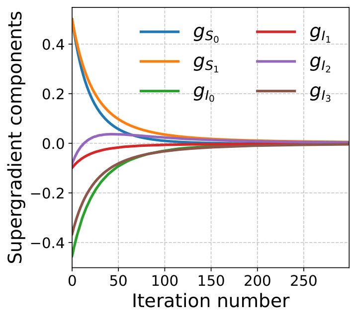 Figure 1
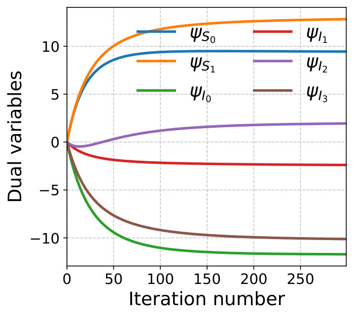 Figure 2
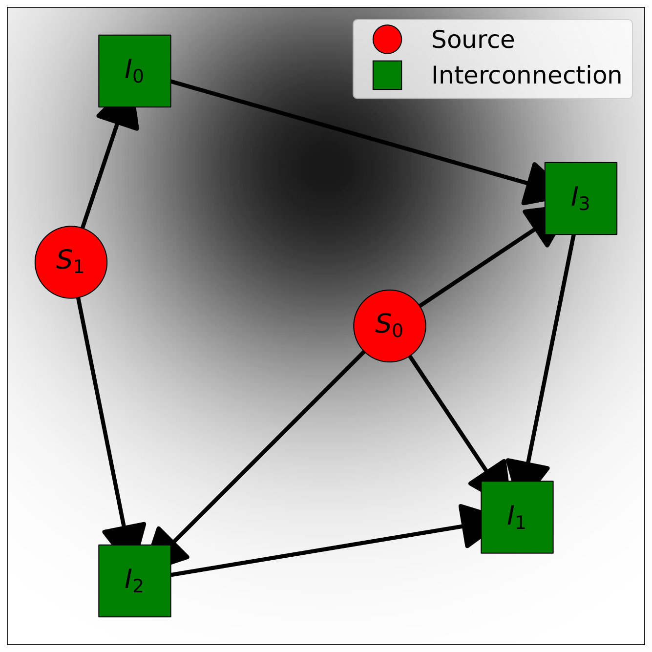 Figure 3
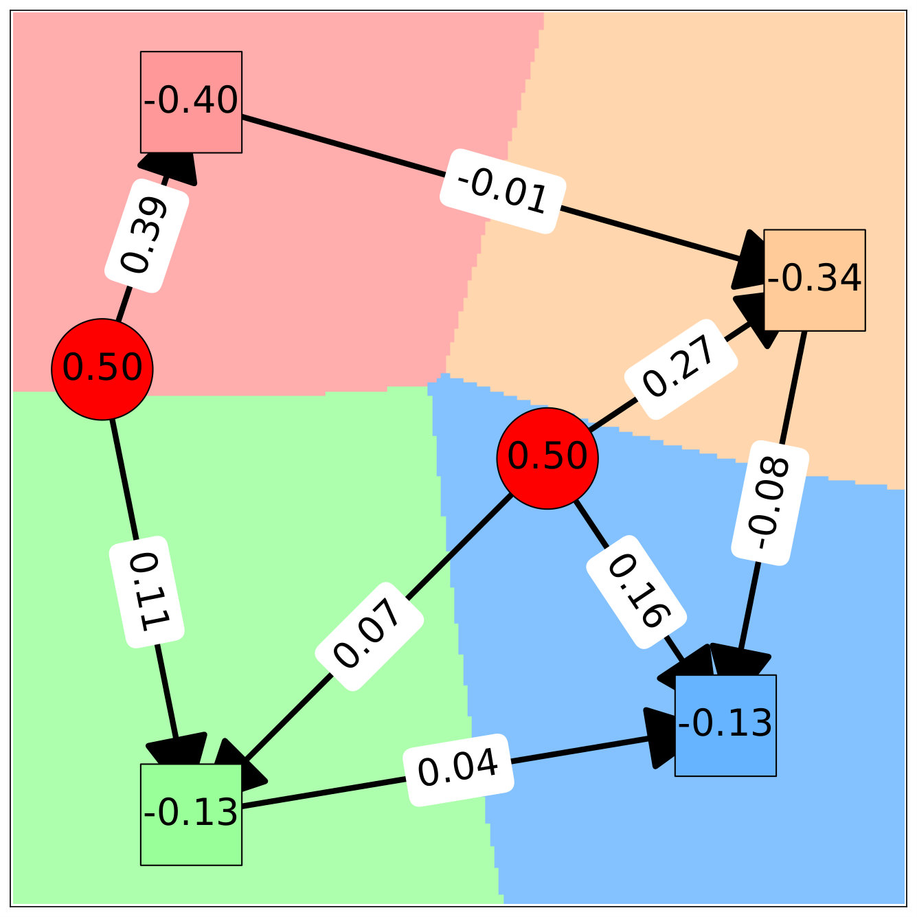 Figure 4
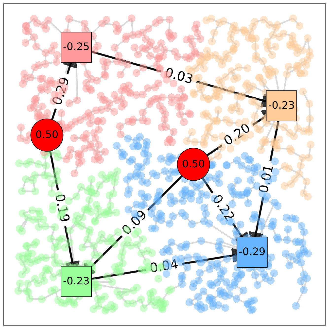 Figure 5
Peer Reviews
No public reviews on file for this paper yet. If you reviewed it on a platform where reviews are public (OpenReview, ICLR, NeurIPS, ICML), you can paste yours below so the community can read it here.
Videos
No videos yet. Explain this paper in a talk, walkthrough, or lecture? Add one.
Taxonomy
TopicsAdvanced Manufacturing and Logistics Optimization
Distributed Combined Space Partitioning and Network Flow Optimization: an Optimal Transport Approach
Théo Laurentin1,2, Patrick Coirault2, Emmanuel Moulay3, Antoine Lesage-Landry1, and Jerome Le Ny1 This work was supported by NSERC under grants ALLRP 586247-23 and RGPIN-5287-2018, and by the Région Nouvelle-Aquitaine under grant AAPR-2023-2022-23896910.1Department of Electrical Engineering, Polytechnique Montreal and GERAD, Montreal, QC H3T 1J4, Canada. Emails: {theo.laurentin, antoine.lesage-landry, jerome.le-ny}@polymtl.ca2LIAS (UR 20299), Université de Poitiers, 2 rue Pierre Brousse, 86073 Poitiers Cedex 9, France. Email: [email protected]3XLIM (UMR CNRS 7252), Université de Poitiers, 11 bd Marie et Pierre Curie, 86962 Futuroscope Chasseneuil Cedex, France. Email: [email protected].
Abstract
This paper studies a combined space partitioning and network flow optimization problem, with applications to large-scale electric power, transportation, or communication systems. In dense wireless networks for instance, one may want to simultaneously optimize the assignment of many spatially distributed users to base stations and route the resulting communication traffic through the backbone network. We formulate the overall problem by coupling a semi-discrete optimal transport (SDOT) problem, capturing the space partitioning component, with a minimum-cost flow problem on a discrete network. This formulation jointly optimizes the assignment of a continuous demand distribution to certain endpoint network nodes and the routing of flows over the network to serve the demand, under capacity constraints. As for SDOT problems, we establish that the formulation of our problem admits a tight relaxation taking the form of an infinite-dimensional linear program, derive its finite-dimensional dual, and prove that strong duality holds. We leverage this theory to design a distributed dual (super)gradient ascent algorithm solving the problem, where nodes in the graph perform computations based solely on locally available information. Simulation results illustrate the algorithm’s performance and its applicability to an electric power distribution network reconfiguration problem.
I Introduction
Optimizing large-scale networks requires solving two fundamental problems: allocating end resources to serve the demand for a product or service, and efficiently routing flows through the network to ultimately meet that demand. For instance, in electric power systems, consumers are assigned to a substation of the distribution system and the necessary power flows are routed through the transmission network to feed the substations. Similarly, in cellular communication networks, users must be matched to base stations and the resulting traffic must be routed through the backbone network. Although the assignment and routing problems are often treated separately for computational efficiency, considering both jointly can improve performance [1, 2].
This work addresses such a combined assignment and flow optimization problem, from an optimal transport (OT) point of view [3, 4]. Specifically, we couple a semi-discrete optimal transport (SDOT) problem [3, Chapter 5] with a minimum-cost flow (MCF) problem [5], and develop a distributed algorithm to solve the combined problem. In the standard SDOT problem, one seeks an optimal transport map from an arbitrary source measure, representing for instance a demand distribution over a geographic area, to a discrete target measure, e.g., a set of endpoint nodes capable of serving this demand. This map in effect partitions the space supporting the demand distribution into different cells, such that the total demand in each cell equals the capacity of the associated endpoint node. Meanwhile, the MCF problem allows us to determine how to route flows efficiently through a network connecting the endpoints to supply nodes, subject to edge capacity constraints.
Problems related to the one formulated in this paper have been considered in several application domains. For example, in electrical distribution networks comprising substations and consumers connected via lines equipped with tie and sectionalizing switches, the radial reconfiguration problem [6], further discussed in Section V-B, aims to selectively open and close switches to form a radial topology, with substations acting both as root nodes of the distribution network and as interfaces to the transmission network where generation is available. This reconfiguration process results in a spatial partitioning that guarantees demand satisfaction while minimizing power losses. Conventional approaches to address it rely on solving computationally difficult mixed-integer programs or use faster heuristics that yield suboptimal solutions [6]. Recent studies have explored clustering [7, 8] and partitioning techniques [9] to mitigate computational challenges, but retain a purely discrete network modelling approach. In contrast, the SDOT framework adopted here can provide good heuristic solutions for asymptotically large distribution networks by considering the limit of a continuous distribution of customers.
In communication networks, related problems combining user association and resource allocation have been formulated as difficult combinatorial problems [2, 10]. Alternatively, SDOT has been used for space partitioning, e.g., for C-RAN device association [11] and communication with UAVs[12]. However, these papers did not integrate network flow optimization. Another related problem is branched optimal transport (BOT) [13], which uses subadditive costs in an OT formulation to encourage mass transport along paths, effectively yielding branched networks. However, in BOT, the backbone network needs to be designed, whereas it is fixed and given here. Moreover, exact methods are limited to small instances and heuristics are generally required [13].
To ensure scalability to large-scale networks, we propose a distributed optimization method to solve our problem, where an agent placed at each node of the backbone network updates its local variables by communicating only with neighbouring agents. Distributed methods for various OT problems have been proposed in recent years. Decentralized alternating direction methods of multipliers (ADMM)-based methods can be used in discrete settings [14], while [15] propose a distributed online optimization and control strategy for a continuous problem. For SDOT, dual deterministic and stochastic gradient ascent methods can be implemented in a distributed manner by computing assignment cell areas exactly or via sampling methods [16, 17]. MCF problems have similarly been solved using distributed auction-based algorithms [18] or distributed dual gradient ascent when cost functions are strictly convex [5]. Under additional regularity conditions, [19] develops a distributed Newton method. The approach proposed here relies on a dual gradient ascent to accommodate both the SDOT and MCF components.
The main contributions of this work are threefold. First, we propose a new framework combining SDOT and MCF, enabling joint space partitioning and flow optimization for the backbone network. Specifically, our model extends SDOT by allowing the target distribution to vary according to network constraints, a significant departure from standard formulations where this distribution is fixed. Second, leveraging optimal transport theory, we derive the dual problem and show that strong duality holds. Third, we develop a distributed dual ascent algorithm to solve the combined SDOT–MCF problem, suitable for large-scale networks.
The rest of this paper is organized as follows. Section II formulates the problem. Section III-A introduces a Kantorovich-type relaxation [4] of the problem, derives its dual, shows that strong duality holds, and that the relaxation is tight. Section IV develops the distributed dual gradient ascent algorithm. Simulation results are presented in Section V, and concluding remarks are provided in Section VI.
II Problem formulation
We now formally define our optimization problem. We consider a space equipped with a non-negative measure , which models, for instance, a demand distribution for a certain product, e.g., electric power, by a population of consumers spatially distributed over . In addition, we consider a network modelled by a directed graph , where is a finite set of nodes and is a set of arcs. Each node has an associated net supply value (with allowed, indicating a demand node). A subset of the nodes, denoted by , corresponds to endpoint stations effectively serving the consumers, e.g., distribution substations in power systems. Serving a unit of demand at by endpoint incurs a cost , where is a given function, taking possibly infinite values. Moreover, the product can travel through the network, e.g., the electric transmission system, with the variables representing the flows along the arcs, where denotes the cardinality of a set. Sending a flow along arc incurs a cost , e.g., corresponding to active power losses, for given functions . Illustrative examples are shown on Figures 1(a) and 3 in Section V.
The overall objective is to simultaneously determine how to assign each consumer of to an endpoint in and route the product through the network, so as to satisfy demand and minimize the combined costs of assignment and routing. A deterministic assignment of consumers in to endpoints in can be described by a map . The total demand assigned to endpoint is then given by , where denotes the pushforward measure of by . The set defines a cell of points assigned to endpoint , and these cells for form a partition of . The combined spatial assignment and network flow optimization problem is then formulated as follows
[TABLE]
where in (1d) the scalars and , for , are lower and upper limits on arc flows, and (1b) and (1c) represent the conservation of flow at each node. In particular, we distinguish between the flow constraints (1b) at the endpoints , which must serve the demand , and the flow constraints (1c) at the other nodes that only route traffic through the network.
In this paper, we make the following assumptions.
Assumption 1**.**
We assume that:
- (a)
The assignment cost function is lower semi-continuous and bounded from below. 2. (b)
The domain is compact. 3. (c)
The arc cost functions are convex and lower semi-continuous for all . 4. (d)
Problem (1) admits a feasible solution.
In Assumption 1, (a) and (b) are standard in the OT literature, with (b) being satisfied in practical applications and useful to simplify technical arguments [4]. Property (c) is necessary to leverage duality results and also standard for MCF problems. Assumption 1-(d) is non-trivial and implies in particular, by summing constraints (1b) and (1c), that we must have , i.e., an equilibrium between demand and supply, in order for the flow conservation constraints to admit a feasible solution.
The objective of this work is to develop an algorithm to solve the optimization problem (1), which moreover admits a distributed implementation by the nodes of the network, i.e., each node should execute operations that only require information exchanges with their neighbours in the graph . In addition, the method of assigning consumers to endpoints should also scale to large-scale problems.
III Characterization of an Optimal Solution
III-A Kantorovich Relaxation and its Dual
From an OT point of view, (1) is a type of Monge problem [4], because the assignment of consumers to endpoints takes the form of a map. For such problems, it is generally useful to introduce the corresponding Kantorovich relaxation, by replacing the transport map with a transport plan , i.e., a non-negative measure on . Intuitively, this change allows for randomized assignments of consumers to endpoints. The relaxed problem reads
[TABLE]
where denotes the -measurable subsets of . Constraint (2c) ensures that is the first marginal of , and in (2b) the quantity represents again the total demand assigned to . Problem (2) is a relaxation of (1), because (1) is obtained by restricting to measures induced by deterministic maps, i.e., of the form , where is the identity map of and .
The benefit of this relaxation is that (2) is now a linear program, although still infinite-dimensional in general, which satisfies useful duality properties [4]. In particular, we establish the following key duality result, whose proof is sketched in Appendix -A.
Theorem 1**.**
Under Assumption 1, the optimal value of (2) is equal to
[TABLE]
where the dual function is given by
[TABLE]
Moreover, the infimum in (2) is attained at an optimal solution .
Note that (3) is a finite-dimensional optimization problem, in contrast to the primal problem (2), a feature that we exploit to design our algorithm in Section IV.
III-B Reconstructing the Primal Optimal Solution
To recover an optimal solution for the original problem (1), we introduce a few additional assumptions. The first is commonly assumed to guarantee the tightness of the Kantorovich relaxation for SDOT problems [16].
Assumption 2**.**
For every pair of distinct nodes and every real number , the set has -measure zero.
Define, for each and , the generalized Laguerre cell [20, 3]
[TABLE]
These cells are used below to define the optimal assignment map. Assumption 2 ensures that the intersection of two distinct Laguerre cells, where assignment randomization could be beneficial, has -measure [math] and hence does not contribute to the overall cost. Note that the Laguerre cells are polytopes when and is the squared Euclidean distance between and the position of node [20]. Next, we introduce the following technical assumption.
Assumption 3**.**
A dual optimal solution maximizing (3) exists.
Explicit conditions under which Assumption 3 is satisfied will be developed in future work. It is empirically satisfied in our numerical simulations in Section V, and it is known to be satisfied for the standard SDOT problem under Assumption 1-(b), see [21, Lemma 9]. Finally, the next assumption, which strengthens Assumption 1, is often made to simplify the analysis of the MCF component of the problem.
Assumption 4**.**
For each arc , the cost function is strictly convex.
Assumption 4 ensures that for all , the minimizer
[TABLE]
exists and is unique. The following proposition provides a means to compute an optimal solution for the original problem (1), assuming an optimal dual solution is known. It also shows that the relaxation (2) is tight.
Proposition 1**.**
Under Assumptions 1, 2, 3, and 4, let be a maximizer of (3), let for each arc , computed from (5), and let be the vector with components . Define the assignment map , for every , with ties between endpoints in the minimization broken arbitrarily, if any. Then, the pair is an optimal solution for (1).
Note that the map in Proposition 1 specifies that all points in should be assigned to endpoint . The proof of this proposition is sketched in Appendix -B.
IV Distributed Algorithm
In this section we propose a distributed algorithm to solve problem (1). Based on the previous analysis, one can compute an optimal dual solution for (3) and then recover an optimal primal solution using Proposition 1.
IV-A Concavity and Supergradient of the Dual Function
In this section we show formally that the dual function (4) is concave, which is expected from duality theory. We also provide an explicit expression for its supergradient, which we exploit later to design a gradient ascent algorithm.
Proposition 2**.**
The dual function defined in (4) is concave. Moreover, under Assumptions 1, 2, and 4, a supergradient at has components, for each ,
[TABLE]
and, for each ,
[TABLE]
Proof.
We decompose the dual function in (4) as , with
[TABLE]
and,
[TABLE]
by analogy with the dual functions for the SDOT problem [16] (without the linear term ) and the MCF problem [5]. Then, is concave as a sum of linear terms and the minimum of affine functions. Under Assumption 4, its supergradient at is given by the expression (7) for each , see [18, Chapter 5.5.]. Moreover, under Assumption 2, we can write
[TABLE]
As shown in [16, Theorem 4], this function is concave and its supergradient at has as component for each . By addition, is concave and its supergradient is given by (6) for each and (7) for each . ∎
IV-B Supergradient Algorithm and Distributed Implementation
Starting from an arbitrary initial value , an iterative supergradient ascent algorithm to maximize (3) takes the form
[TABLE]
with given in Proposition 2 and the positive scalar stepsizes satisfying the standard conditions
[TABLE]
Under these conditions, and noting that the gradients in Proposition 2 are uniformly bounded, the sequence converges to an optimal value of (3) as . Moreover, under Assumption 3, the iterates also converge to an optimal solution [22, Proposition 8.2.6], which can then be used to compute the assignments and flows using Proposition 1. We can now describe a distributed method to solve problem (1), outlined in Algorithm 1.
Assume that a computing agent at each node within the network updates the dual variable according to (8), for which it needs to compute the supergradient component given in Proposition 2. At each iteration the agents compute the current flows on Lines 5-7 by exchanging information only with their outgoing and incoming neighbours. For endpoint nodes , an additional step on Line 9 is required to determine the measure of its current Laguerre cell in order to compute the supergradient component (6). This step depends a priori on the variables of possibly all the other endpoints . Most practical instances feature a finite set of customers and a discrete measure encoding their individual demands. At iteration , each endpoint needs to compare the adjusted costs with those of the other endpoints. A customer at is matched to the endpoint that offers the lowest value. Then, we can compute the total demand of the customers lying in the Laguerre cell of . For some cost functions , e.g., the squared distance between and the position of node , the geometric properties of the Laguerre cells can be exploited so that an endpoint only needs to compare the adjusted costs with other endpoints that share a cell boundary with it, see, e.g., [23].
Remark 1**.**
The discretization of the space to compute the masses deterministically can be replaced by a stochastic integration method, generating samples according to for which the endpoints then compare their adjusted costs, as discussed in [16] for SDOT. The iterates (8) then become a stochastic gradient algorithm, again with convergence guarantees.
Finally, the agents need to detect convergence in a distributed manner. A possible test used on Line 15 is that each node stops updating its dual variable when its variation stays below a certain threshold . Each agent may also wait until the variables of its neighbours have converged as well before recomputing the final flows (as on Line 6) and Laguerre cells. Regarding the assignment computation, each endpoint can determine the points belonging to its Laguerre cell. Alternatively in some applications, the final weights can be broadcast to the customers, who can then determine their assigned endpoint automatically.
V Numerical Simulations
In this section, we illustrate our method through two numerical examples. First, we test Algorithm 1 on a synthetic example. Second, we briefly explore the applicability of the method to a more complex scenario relevant to electric power distribution networks.
V-A Synthetic Example
We first consider a simple scenario shown on Figure 1(a), defined on a square domain of side length . A continuous consumer demand distribution is discretized on a grid, for a total of 40,000 points. Each consumer is assigned a mass from a truncated Gaussian density with mean and standard deviation . The backbone network consists of two nodes with a supply , called source nodes, and four nodes with zero supply, called interconnection nodes. Node positions and arcs are also shown on Figure 1(a).
The assignment cost between consumer demand at and node is given by the Euclidean distance between and the position of node . The arc costs are assumed to be quadratic functions of the flows, i.e., , where is the Euclidean distance between nodes and . We assume and for all , and obtain the closed-form local flow update at Line 6 of Algorithm 1 given by . The algorithm is run for iterations with diminishing step-size . Figure 2 shows the convergence of the components of the supergradient toward zero and of the dual variables . Figure 1(b) illustrates the resulting routing and partitioning solutions. Each cell is coloured according to its assigned endpoint node, and the network is represented with annotated flows on its arcs. Source nodes are labelled with their fixed supply , and endpoints display their assigned demand
V-B Electric Power Network Example
We now discuss an application to an electrical power network consisting of a transmission system linking generators to substations and a distribution network connecting substations to consumers. Consumer demand, initially discrete, is approximated by a continuous distribution. Substations are endpoint nodes in our formulation.
An important problem in electrical networks is the radial reconfiguration of the distribution network: activating or deactivating switches on lines to ensure that each consumer is served via exactly one distribution path to a unique substation, forming tree-like (radial) subnetworks rooted at substations, see Figure 3. Solving large-scale reconfiguration problems exactly is computationally challenging [6], so that the coupling with the transmission network optimization problem is usually neglected. Here we use Algorithm 1 to develop a heuristic producing an initial assignment of customers to substations while minimizing transmission costs. This enables subsequent parallelized radial reconfiguration per substation, greatly reducing the computational burden.
We assume that the arc costs on the transmission network are , representing power losses, where is the line resistance and is the power flow. We take as the distance in this example. Next, to approximately capture the power losses in the distribution network through the simple assignment cost , we choose for the geodesic (shortest‑path) resistance through this network between a customer and the substation . The quality of this heuristic choice will be explored in future work. This choice also ensures an essential connectivity property for the resulting Laguerre cells: all consumers assigned to a substation can be physically connected to it via paths lying entirely within their assigned cell. Briefly, if a consumer belongs to the Laguerre cell associated with substation and vector , all intermediate nodes along the shortest path from to also belongs to . This follows directly from the definitions of Laguerre cells and shortest paths, because for all :
[TABLE]
which implies , hence .
Figure 3 illustrates the partitioning and routing solutions obtained for this power network example. The transmission network topology mirrors the synthetic example described in Section V-A. The distribution network was generated by randomly placing 1000 consumer nodes within the domain, each assigned a uniformly random demand value. To ensure a realistic network structure, each consumer node was connected to its two or three geographically closest neighbours. Figure 3 displays the resulting Laguerre cells, with consumer nodes coloured according to their assigned substation, alongside optimized flows within the transmission network. The algorithm parameters used match those of the synthetic example.
VI Conclusion
We have studied a combined space partitioning and network flow optimization problem motivated by the operation of large-scale networks serving spatially distributed consumers. By adopting an optimal transport perspective, we derived a dual formulation and designed a distributed algorithm relying only on local information exchanges. Numerical experiments confirmed the effectiveness of the method and illustrated its relevance to power distribution network reconfiguration. Future work will investigate extensions of the framework, in particular incorporating flexible generation through additional decision variables at network nodes.
-A Proof Sketch of Theorem 1
Theorem 1 can be proved by following a general methodology for OT problems, as in [4, Theorem 1.3]. Recall that for any function on a normed vector space with dual , its conjugate is defined by
The methodology relies on the following version of the Fenchel–Rockafellar duality theorem [4, Theorem 1.9].
Theorem 2** (Fenchel–Rockafellar).**
Let be a normed vector space and its dual. If are convex functions and if there exists such that and are finite and is continuous at , then
[TABLE]
To prove Theorem 1, we define suitable convex functions and on a suitable space and apply Theorem 2. In our case, we take , where denotes the space of continuous bounded functions on equipped with the supremum norm. By Riesz’s theorem, its topological dual space can be identified with the space of finite signed Radon measures on , denoted by . Thus, the dual space is , with the duality pairing between and given by
[TABLE]
We then define , where
[TABLE]
as in [4], and , with
As for the function , extending the idea in [4, Theorem 1.3], if there exist functions and such that for all for all , then
[TABLE]
otherwise, we set . The function is well-defined [4, p. 27]. With some sign changes in the variable definitions, we have that
[TABLE]
Next, after some calculations, leveraging under Assumption 1-(c) (convexity), we can show that
[TABLE]
provided that , and , i.e., matching (2a) under (2d), and otherwise. For , by reparameterizing any with finite in terms of and , one obtains that enforces the marginal condition for all (see (2c)) and the flow balance constraints (see (2b)); that is, if these conditions hold and otherwise.
It follows that is exactly the negative of the primal problem (2). Thus, by applying Theorem 2 we obtain the desired duality result. Assumption 1, with the key hypotheses that and are lower semicontinuous and convex, is compact, and the feasibility condition , ensures that and satisfy the convexity, continuity and qualification conditions required to apply the theorem.
-B Proof Sketch of Proposition 1
Let be an optimal solution for (2) and be an optimal dual solution for (3). Since is feasible, the flow constraints hold, so by multiplying each constraint in the primal problem by and using strong duality, we have
[TABLE]
Substituting by its definition (4) and bringing all the terms to the right-hand side, the terms vanish and we obtain , with
[TABLE]
and, using the marginal constraint (2c). Now, because and , each term must be zero.
For the flow terms, for every arc implies , i.e., the minimizer in (5) for . For the integral term, we must have -almost everywhere that , i.e., is concentrated on the set
[TABLE]
Hence, for -almost all , when the minimizing index is unique must assign to , which corresponds to the map in Proposition 1. When the minimizer is not unique, may randomize between them, however under Assumption 2, choosing the deterministic assignment also for such has no impact on the cost. Overall, this shows that and is optimal for (2), so is optimal for (1) and the relaxation is tight.
The reference list from the paper itself. Each links out to its DOI / PubMed record.
- 1[1] A. G. Givisiez, K. Petrou, and L. F. Ochoa, “A review on tso-dso coordination models and solution techniques,” Electric Power Systems Research , vol. 189, 2020.
- 2[2] D. Fooladivanda and C. Rosenberg, “Joint resource allocation and user association for heterogeneous wireless cellular networks,” IEEE Transactions on Wireless Communications , vol. 12, no. 1, pp. 248–257, 2012.
- 3[3] G. Peyré and M. Cuturi, “Computational optimal transport: With applications to data science,” Foundations and Trends in Machine Learning , vol. 11, no. 5-6, 2019.
- 4[4] C. Villani, Topics in Optimal Transportation . AMS, 2003.
- 5[5] D. Bertsekas, Network Optimization: Continuous and Discrete Methods . Athena Scientific, 1998.
- 6[6] H. Lotfi, M. E. Hajiabadi, and H. Parsadust, “Power distribution network reconfiguration techniques: A thorough review,” Sustainability , vol. 16, no. 23, 2024.
- 7[7] R. J. Sánchez-García, M. Fennelly, S. Norris, N. Wright, G. Niblo, J. Brodzki, and J. W. Bialek, “Hierarchical spectral clustering of power grids,” IEEE Transactions on Power Systems , vol. 29, no. 5, pp. 2229–2237, 2014.
- 8[8] E. C. Pereira, C. H. N. R. Barbosa, and J. A. Vasconcelos, “Distribution network reconfiguration using iterative branch exchange and clustering technique,” Energies , vol. 16, no. 5, 2023.