Boundary Stabilization of a Bending and Twisting Wing by Linear Quadratic Gaussian Theory
Arthur J. Krener

TL;DR
This paper develops a boundary stabilization method for a cantilever wing's bending and twisting using an infinite-dimensional LQR approach combined with a Kalman filter, incorporating aerodynamic forces based on Wagner's function.
Contribution
It introduces a novel boundary control and estimation framework for wing stabilization using infinite-dimensional LQR and Kalman filtering with aerodynamic modeling.
Findings
Effective boundary stabilization achieved for bending and twisting modes.
Integration of aerodynamic forces into the control model.
Demonstrated feasibility of the approach for high aspect ratio wings.
Abstract
We first consider the stabilization of the bending and twisting of a rectangular cantilever beam of moderate to high aspect ratio using full state feedback boundary control. Our approach is an infinite dimesnional extension of Linear Quadratic Regulation (LQR). The we develop an infinite dimensional Kalman filter that processes two point measurements and returns an estimate of the full state. The Linear Quadartuc Gaussian approach is to use this estimate in the place of the full state in the LQR feedback Then we add aerodynamic forces to obtain a model of a wing. The aerodyamic model is based on a two dimensional state space approximate realiztion of Wagner's indicial function by R.~T.~Jones.
Click any figure to enlarge with its caption.
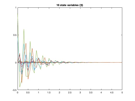 Figure 1
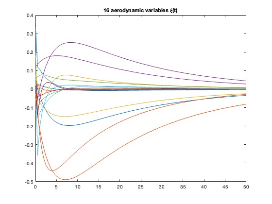 Figure 2
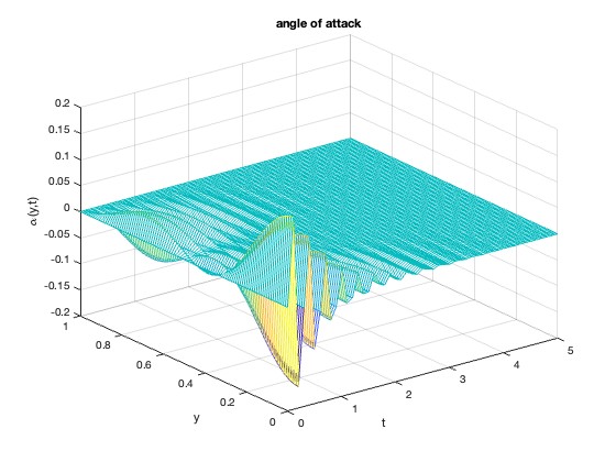 Figure 3
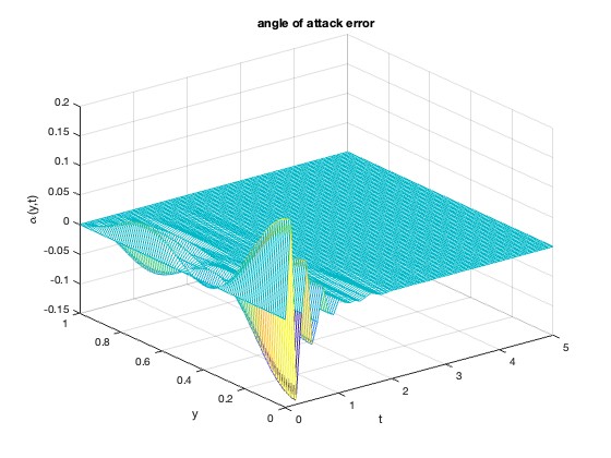 Figure 4
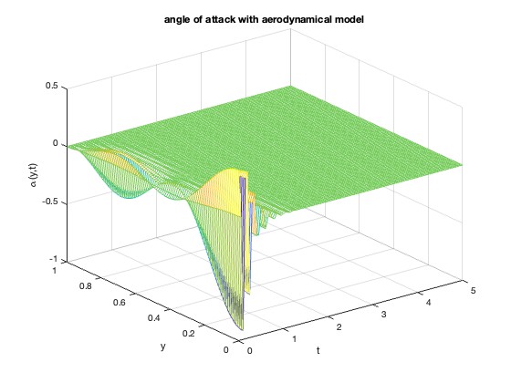 Figure 5
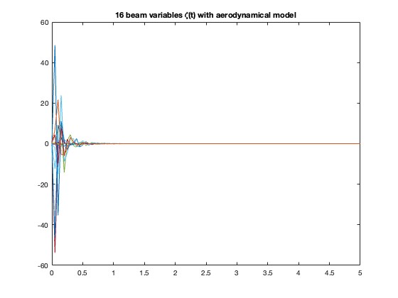 Figure 6
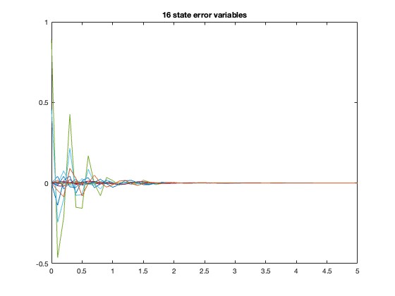 Figure 7
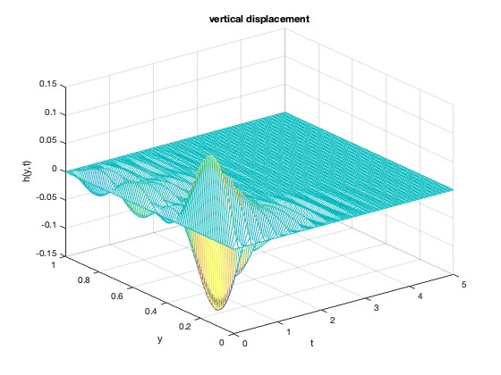 Figure 8
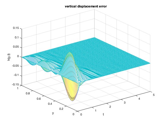 Figure 9
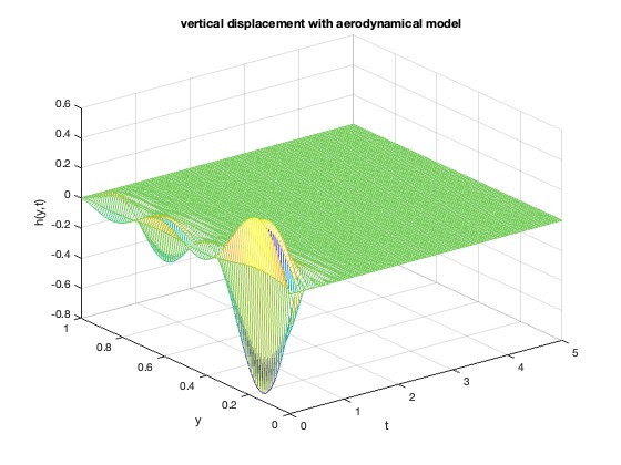 Figure 10
Peer Reviews
No public reviews on file for this paper yet. If you reviewed it on a platform where reviews are public (OpenReview, ICLR, NeurIPS, ICML), you can paste yours below so the community can read it here.
Videos
No videos yet. Explain this paper in a talk, walkthrough, or lecture? Add one.
Taxonomy
TopicsStability and Controllability of Differential Equations · Aeroelasticity and Vibration Control · Control and Stability of Dynamical Systems
Boundary Stabilization of a
Bending and Twisting Wing
by Linear Quadratic Gaussian Theory
Arthur J. Krener This work was funded by AFOSR under grant FA9550-23-1-0318.A. J. Krener is with the Department of Mathematics, University of California, Davis, CA 95616 , USA, [email protected].
Abstract
We first consider the stabilization of the bending and twisting of a rectangular cantilever beam of moderate to high aspect ratio using full state feedback boundary control. Our approach is an infinite dimesnional extension of Linear Quadratic Regulation (LQR). The we develop an infinite dimensional Kalman filter that processes two point measurements and returns an estimate of the full state. The Linear Quadartuc Gaussian approach is to use this estimate in the place of the full state in the LQR feedback Then we add aerodynamic forces to obtain a model of a wing. The aerodyamic model is based on a two dimensional state space approximate realiztion of Wagner’s indicial function by R. T. Jones.
I Introduction
High Altitude Long Endurance (HALE) aircraft have highly flexible wings. Helicopter blades are also highly flexible. One would like to use active control to dampen their oscillations. One can model a wing by the beam equation or the plate equation. In [7] it is stated that ”even for relatively low aspect ratios of thin rectangular cantilever plates, the model based on the beam theory is closer to (our) experimental model (as) compared to the plate theory.” So we choose a model based on the beam equation.
We assume that the beam can bend and twist and that there are two point actuators, one can deliver a bending moment to the root of the beam and the other can deliver a torque also at the root of the beam. We also assume that there are two point sensors, one measures the vertical velocity of the tip of the beam and other measures the angular velocity of the tip of the beam. We wish to design a compensator that processes the measurements and delivers a bending moment and torque that dampens the bending and torsion oscillations. We design this compensator using Linear Quadratic Gaussian (LQG) theory. After accomplishing this we convert the model of the beam into a model of a wing by adding the aerodynamic forces that the motions of the beam generate. We model the aerodynamic forces by a state space approximate realization of the classical indicial function of Wagner. Wagner’s indicial function is for an airfoil, a cross section of a wing, but we extend it to the whole wing.
Linear Quadratic Gaussian (LQG) theory is a well-known way of designing a dynamic compensator for a controlled and observed finite dimensional dynamical system. We extend LQG to designing a dynamic compensator for a controlled and observed infinite dimensional dynamical system under point actuation and point sensing. The LQG approach breaks the problem into two parts. The first part uses Linear Quadratic Regulator theory to find a stabilizing linear feedback. This feedback assumes that exact measuremnts of the full state are available. In most situations this assumption is unrealistic. The second part is to design a Kalman filter that processes the noisey measurements and returns an estimate of the full state. This estimate is used in place of actual state in the linear feedback. The result is a dynamic compenstor. The closed loop eigevalues of the combined system are the union of the eigenvalues of system under full state feedbck and the eigenvalues of the error dynamics of the Kalman filter. If all these eigevalues lie in the open left plane then the combined plant and Kalman filter is asymptotically stabe.
We start with the model presented in Section 3.6 of the classic treatise of Bisplinghoff, Ashley and Halfman, [2]. This is a linear model which ignores the nonlinear interactions between the bending and the torsion of the rectangular beam. We add point actuation and point sensing to the boundary of the model. Point actuation and point sensing are idealizations of actuation and sensing over small domains on the boundary and the idealization simplifies the mathematical analysis.
The linear model is neutrally stable so the bending and the torsion oscillations do not decay. We seek a compensator to asymptotically stabilize these oscillations. A model for designing a stabilizing compensator does not need to be as accurate as a model for simulation because any errors will decay during the stabilization process.
To the model of [2] we add two actuators located where the horizontal beam is joined to its support. One actuator affects the bending of the beam at its support and other affects the torsion of the beam at its support. We first seek a state feedback control law which drives the oscillations to zero. To find such a feedback we set up and solve a Linear Quadratic Regulator (LQR). We are certainly not the first to use LQR to find a state feedback that stabilizes a bending and twisting beam. Edwards, Breakwell and Bryson [5] used LQR to find a state feedback that stabilizes an airfoil, a cross section of a wing, using leading edge and trailing edge flaps. We stabilize the whole beam with two actuators at the root of the beam.
This work was presented at 2025 American Control Conference in Denver, CO and is repeated here because it is necessary background for the additinal material, the Kalman filter and aerodynamic model, that we present here. We add two sensors to the model, one which measures the vertical velocity at the tip of the wing and other that measures the rate of torsion also at the tip of the wing. We design a Kalman filter to process these measurements and return an estimate of the full state.
Finally we add a model of the aerodynamics forces that a bending and twisting beam generates to obtain a model of a wing. The model is based on the classic Wagner model for the aerodynamic forces exprienced by an airfoil in flight as described in [3]. We extend a standard finite dimensional model of an airfoil to a model of the complete wing and expand it using the same families of eigenfunctions that were used to describe the bending and twisting of the beam.
We present several simulations of the beam and wing to demonstrate the effectiveness of our approach.
II Dynamical System
Let the axis be the axis of rotation of the beam and suppose it extends from where it is attached to its support and its free end is at . Let be the vertical deflection of beam at location and time and let be the angle of rotation of the beam around the axis at location and time . According to [2], equations (3-155) and (3-156), the free vibrations of a uniform beam are governed by the two inertially coupled linear PDEs
[TABLE]
where
[TABLE]
The inertial coupling coefficient is zero if all the centers of gravity of the cross sections lie on the elastic axis.
The bending boundary conditions at the free end of the beam are
[TABLE]
and at the fixed end of the beam we assume that there is an actuator that can deliver a bending moment
[TABLE]
The torsion boundary condition at the free end of the beam is
[TABLE]
and at the fixed end of the beam we assume that there is an actuator that can deliver a torque
[TABLE]
We define
[TABLE]
We wish to express the dynamics as a first order system so we introduce a four vector valued variable
[TABLE]
then (7) becomes
[TABLE]
where
[TABLE]
The boundary conditions on are
[TABLE]
We seek a feedback law of the form
[TABLE]
to stabilize the bending and torsion oscillations so we set up a Linear Quadratic Regulator (LQR). We choose a nonnegative definite matrix valued function that is symmetric in its arguments, and a positive definite matrix . For a given initial condition we seek to minimize by choice of the quantity
[TABLE]
where is the square and .
Let be an nonnegative definite matrix valued function that is symmetric in its arguments, and satisfies these homogeneous boundary conditions for
[TABLE]
These boundary conditions are analogous to the those on when the the controls are zero and will be important when we integrate by parts below. We assume that the are so that these boundary conditions make sense.
LQR requires a stabilizability condition so we assume that for each there is a such that and as . Then by the Fundamental Theorem of Calculus
[TABLE]
LQR also requires a detectability condition so we assume that if is such that
[TABLE]
then as .
We bring the time differentiation inside the spatial integrals and integrate by parts several times to obtain
[TABLE]
where and denote the row and the column of respectively.
We add the right side of (233) to the criterion (22) to get an equivalent criterion to be minimized. We wish to find a matrix valued function such that the time integrand of equivalent criterion is equal to a perfect square of the form
[TABLE]
The terms quadratic in match so we equate terms bilinear in and . This yields
[TABLE]
so we assume that
[TABLE]
By symmetry
[TABLE]
Then by equating terms bilinear in and we obtain the Riccati PDE for quadratic Fredholm kernel of the optimal cost,
[TABLE]
where . This is an elliptic PDE with a quadratic nonlinearity.
III Fourier Analysis
We solve the Riccati PDE (54) by Fourier series. The partial differential operator is self adjoint under the zero controlled boundary conditions
[TABLE]
so all the eigenvalues are real and the eigenfunctions are orthogonal. The eigenfunctions are and the eigenvalues are for .
These are not the eigenpairs of the wave equation under the boundary conditions (60) but are related to them. The eigenpairs of the wave equation
[TABLE]
when written as a first order system are which are strictly imaginary if . The corresponding eigenfunctions are
[TABLE]
The partial differential operator is self-adjoint when subject to the boundary conditions
[TABLE]
Note that these are not the boundary conditions of a cantilever beam. For a cantilever beam, the second boundary condition is , not
We look for eigenpairs that satisfy
[TABLE]
and the boundary conditions (62).
Also note that an eigenpair satisfying (63) and (62) is not an eigenpair of beam equation
[TABLE]
but it is related to them. When written as a first order system the beam eigenpairs are the eigenpairs of the matrix differential operator
[TABLE]
The beam eigenvalues are and since the beam eigenvalues are strictly imaginary. The corresponding beam eigenfunctions are vector valued,
[TABLE]
Because the differential operator is self-adjoint under the zero controlled boundary conditions (62) it follows that all its eigenvalues are real and there is an orthogonal family of eigenfunctions, . Regardless of the boundary conditions, any eigenfunction of the partial differential operator must be of the form
[TABLE]
for some real . Then the eigenvalue is . We can express the boundary equations as a set of homogeneous linear equations depending on ,
[TABLE]
This system has a nontrivial solution iff is a root of the determinant of this matrix. The determinant is
[TABLE]
By adjusting the signs of and we can restrict our attention to nonnegative roots. There is no nonzero eigenfunction corresponding to so it is not an eigenvalue. The positive roots occur when . For each there is exactly one root . The first four roots are , , , . As the root is quickly converging to .
Because of the boundary conditions (62) at we look for eigenfunctions are of the form
[TABLE]
Without loss of generality we can take . Then the boundary conditions (62) at imply
[TABLE]
or equivalently
[TABLE]
For large we have so we conclude that for large , . This happens when .
So the eigenfunctions are converging to .
[TABLE]
and
[TABLE]
We conjecture that the set of vectors is a Riesz basis for .
IV Series Solution of the Riccati PDE
Suppose has an expansion of the form
[TABLE]
We could consider more general but to keep the exposition relatively simple we do not. Notice that the ranges of the sums are different.
We also assume that the solution of the Riccati PDE (54) has a similar but more complicated expansion.
[TABLE]
Note we are abusing notation, is not necessarily the same as even when and . We use as a superscipt to indicate a coefficient of and we use as a superscipt to indicate a coefficient of .
We plug these expansions into Riccati PDE and collect similar terms to obtain an infinite dimensional algebraic Riccati equation which has four uncoupled components. The component is
[TABLE]
The component is
[TABLE]
A simple solution to this equation is to take for all and . Then by symmetry . This would not be possible if we had chosen .
Finally the component is
[TABLE]
V Policy Iteration
We can approximately solve the algebraic Riccati equations (93) and (128) by policy iteration. The method can also be seen as value iteration. To find an initial iterate and we make the following assumptions.
if or . 2. 2.
if when . 3. 3.
if or . 4. 4.
if when .
These assumptions decouple bending from twisting so the four dimensional equations (93) and (128) reduce to two independent two dimensional equations. The Fourier expansion of the bending model is solely in terms and it satisfies
[TABLE]
Recall as .
The Fourier expansion of the twisting model is solely in terms of and it satisfies
[TABLE]
The above assumptions on the initial iterate simplifies (137) to
[TABLE]
and simplifies (151) to
[TABLE]
Notice the component of (165) is a quadratic equation in ,
[TABLE]
Since it is harder to stabilize when and have the same sign we take the positive root of this quadratic to be the initial estimate
[TABLE]
The component of (165) is a quadratic equation in
[TABLE]
and since must be nonnegative we define
[TABLE]
We can use the or the component of (165) to define . Both lead to
[TABLE]
Then our initial iterate of the kernel of the bending part of the optimal cost is
[TABLE]
Theorem 1: The series (198) converges to a continuous matrix valued function. if there exist numbers and such that
[TABLE]
or .
In addition if for some integer
[TABLE]
or . then the series (198) converges to a matrix valued function.
Proof: The Mean Value Theorem applied to the function on the interval implies that there is an in such that
[TABLE]
Let and . Then so there exists an between and such that
[TABLE]
The maximum of the right side of this equation between and occurs at so
[TABLE]
Since , with and the series
[TABLE]
converges uniformly to a continuous function .
Now by (70) so
[TABLE]
which is . Since the series
[TABLE]
converges uniformly to a continuous function .
Finally
[TABLE]
so and the series
[TABLE]
converges uniformly to a continuous function because .
The assertion (200) is obtained by term by term differentiation of the series (198). QED
The way we interpret this result is that if we want the cost of moving the infinite number of imaginary eigenvalues into the open left half plane to be finite we must make go to zero quite rapidly.
Notice the component of (179) is a quadratic equation in
[TABLE]
Since it is harder to stabilize when and have the same sign we take the positive root of this quadratic to be the initial estimate
[TABLE]
The component of (179) is a quadratic equation in
[TABLE]
and since must be nonnegative we define
[TABLE]
We can use the or the component of (179) to define . Both lead to
[TABLE]
Our initial iterate of the kernel of the twisting part of the optimal cost is
[TABLE]
Theorem 2: The series (208) converges to a continuous matrix valued function if there exist numbers and such that for
[TABLE]
.
In addition if for some integer
[TABLE]
or . then the series (208) converges to a matrix valued function.
Proof: Since the Mean Value Theorem applied to (202) implies that there is an between and such that
[TABLE]
The maximum of the right side of this equation occurs at so we conclude that
[TABLE]
and is of order . Since the series
[TABLE]
converges uniformly to a continuous function.
Now from (204) we know that is of order so the series
[TABLE]
converges uniformly to a continuous function.
Finally from (205) we see that is of order and since we have so the series
[TABLE]
converges uniformly to a continuous function.
The statement (210) is obtained by term by term differentiation of the series (208). QED
Succesive iterates are found by plugging and into the right sides of the algebraic Riccati equations (93) and (128) and solving for and on the left side. A complication arises when because then and so the left sides is not an invertible expression in and . A way around this is for all to plug and into the right sides of the algebraic Riccati equations (93) and (128) and solve for , and for all and all such that . Then plug these iterates into (93) and (128) and solve the resulting quadratics for and when . If the resulting quadratics do not determine and when just set them to zero. It should be noted that if then the approximations to the bending and twisting kernels are not like (198) and (208) but are when .
This is value (or policy) iteration so we know that the iterates are nonincreasing. If hypotheses of Theorems 1 and 2 are satisfied then the initial approximations (198) and (208) are continuous hence bounded on . Hence the initial estimate of the optimal cost is bounded as are all successive estimates. From this we conclude that all of the approximations to the optimal feedback move all the closed loop eigenvalues into the open left half plane. But we cannot conclude that the closed loop system is exponentially stable because the closed loop eigenvalues could (and do) approach the imaginary axis as the wave numbers and increase.
VI Finite Dimensional Approximating LQR
We construct a finite dimensional LQR whose algebraic Riccati equation is a truncation of (93) and (128). We choose an and construct a linear system with state where is each of dimension . So the finite dimensional state is of dimension . The dynamics is
[TABLE]
where
[TABLE]
This finite dimensional system approximates the infinite dimensional system in the following manner
[TABLE]
VII Example
We consider a example which leads to a dimensional approximation. For the time being we take all constants equal except , a identity matrix and a identity matrix. The open and closed loop poles are
[TABLE]
Notice how close the imaginary parts of the closed loop poles are to the open loop poles, All the closed loop poles have real parts less than .
Figure 1 is a simulation of the dimesional state under full state feedabck
Figure 2 shows the vertical displacement converging to zero under full state feedback. The control input at the root of the beam causes the ripples while stabilizing the vertical displacement of the beam.
Figure 3 shows the stabilization of the angle of attack under full state feedback.
Again the control input at the root of the beam causes the ripples while stabilizing the torsion of the beam.
VIII Kalman Filter
In the above sections we have constructed a full state feedback to asymptotically stabilize the linear system. But we don’t have the ability to measure the full state so need to construct a Kalman filter to deliver an estimate of the full state from a finite number of point measurements. We assume that we can measure and . We could use more sensors and/or different types of sensors but to keep thing simple we do not do so.
To develop the Kalman filter it is simpler to express the inertially coupled bending and twisting dynamics in a more standard form by multiplying the dynamics by the inverse of the coupling matrix . We also add a distributed driving noise input and obtain
[TABLE]
where the matrix partial differential operator is and
[TABLE]
The boundary conditions on are
[TABLE]
The measurements are the vertical velocity and angular velocity of the tip of the beam corrupted by white Gaussian noise,
[TABLE]
where
[TABLE]
and is a invertible matrix with standard independent white Gaussian noises. One way of obtaining such measurements is to integrate a pair of accelerometers as was done by Banks et al.[1].
Because of the Gaussian and linear assumptions we expect that when the optimal least squares estimate of is a linear functional of the past observations,
[TABLE]
for some matrix valued function . Notice that depends on the location because we are trying to estimate .
Given such a for each we define a matrix valued function by the differential equation
[TABLE]
The subscript on indicates that it is involves partial differentiation with respect to not .
This PDE is subject to the homogeneous boundary conditions
[TABLE]
and the initial condition
[TABLE]
Then
[TABLE]
Note the parenthesis around . The parenthesis implies that we apply the matrix partial differential operator to before doing anything else with this term.
Now we integrate by parts with respect to
[TABLE]
We expect that the state in the far past to be irrelevant to the estimate of the state at time so we assume that as . Hence
[TABLE]
Then we integrate by parts with respect to using the boundary conditions
[TABLE]
Putting this all together yields
[TABLE]
So the estimation error is given by
[TABLE]
Because and are standard white Gaussian noises, the covariance of the error is
[TABLE]
For each and for each pair of corresponding rows of and we have an LQR in adjoint form with state , control , linear dynamics (229) and a quadratic criterion (232). We can leave this adjoint LQR in matrix form as the optmal feedback gain is the same for all rows,
[TABLE]
That is not to say that the rows of are all the same because the rows of can be different, We are trying to estimate which is why and might depand on .
For each let be a continuous matrix value function of satisfying the homogeneous boundary conditions
[TABLE]
Using the Fundamental Theorem of Calculus assuming as we have
[TABLE]
We formally integrate by parts as if were in
[TABLE]
which reduces to
[TABLE]
We add the right side of (234) to the criterion (VIII) to be minimized to get an equivalent criterion
[TABLE]
We seek a such that the time integrand in (VIII) is a perfect square of the form
[TABLE]
The terms quadratic in match so we equate terms bilinear in and and obtain
[TABLE]
so we set
[TABLE]
Finally we match terms bilinear in and which yields the Riccati PDE of the infinite dimensional Kalman filter
[TABLE]
Actually this is a family of Riccati PDEs paramterized by ,
The optimal estimate is given by
[TABLE]
We make the substitution then
[TABLE]
We differentiate this with respect and obtain
[TABLE]
Then
[TABLE]
where is the differential operator
[TABLE]
Put another way
[TABLE]
and so for each
[TABLE]
We differentiate this with respect to and obtain
[TABLE]
so we conclude that
[TABLE]
and
[TABLE]
We differentiate the optimal estimate with respect and obtain
[TABLE]
so we conclude that
[TABLE]
or
[TABLE]
The boundary conditions on are the same as those (225) on ,
[TABLE]
The so called innovations process is
[TABLE]
where
[TABLE]
This is the difference between the actual observation and what we thing it should be given our optimal estimate of the state.
We can express the optimal filter as a copy of the original dynamics driven by the innovations
[TABLE]
subject to the boundary conditions (259).
If we use the estimate in place of the full state in the feedback law we found before then the control input is
[TABLE]
We insert into the plant boundary conditions (20). We also insert it into the boundary conditions (259) of the Kalman filter. This is dynamic compensation.
The error dynamics is given by
[TABLE]
subject to the homogeneous boundary conditions
[TABLE]
Notice that the error dynamics and its boundary conditions only depend on the error so we can express the combined plant and Kalman filter in the coordinates and . In these coordinates the combined system is upper triangular so if the full state feedback aymptotically stabilizes the system and if the error dynamics of the Kalman filter is asymptotically stable then the dynamic compensator stabilizes the system.
If the coefficient of the driving noise does not depend on , then the family of LQRs does not depend on . Therefore , , and . The optimal filter is given by
[TABLE]
IX Filter Example
We apply the Kalman filter to the dimensional example that we treated above. The error variables are shown in Figure 4.
The vertical displacement error is shown in Figure 5 and the rotational displacement error is shown in Figure 6
Notice that the estimation errors are smaller near the sensors at the tip, .
X Aerodynamic Model
The next step is to add a model of the aerodynamical forces that are generated by the bending and twisting beam to get a model of a wing.The classical aerodynamical models are those of Wagner and Theodoresen. Wagner’s model is in the time domain and Theodoresen’s is in the frequency domain. They are related by the Laplace transform.
These models are not exactly realizable by a linear time invariant system. But over the years considerable effort has gone into finding linear time invariant systems whose impulse response or transfer function approximates Wagner’s or Theodoresn’s model. We shall use the approximation to Wagner’s model developed by R. T. Jones in 1938 as reported in [3]. Wagner’s model is valid for an airfoil, a wing section. We shall extend it to model a wing by introducing spanwise dependence.
The state space realization of Wagner’s model adds two additional states to our four dimensional model. Of course each of these six state variables is a function of and .
Aerodynamical models are parameterized by the free stream air velocity which we could treat as a static state. But then the model would become nonlinear so we do not do so..
Here is R.T. Jones’ approximate state space realization of Wagner’s impulse response. The aerodynamics state is and its dynamics is
[TABLE]
where
[TABLE]
The aerodynamic input is
[TABLE]
The aerodynamics output is
[TABLE]
where
[TABLE]
The lift per unit span is
[TABLE]
The moment per unit span is
[TABLE]
where is the aerodynamic output.
Typical parameter values are
[TABLE]
The model is from [6] and the parameters are from [3].
We conjectured that the combination of and constitutes a Riesz basis for . We expand the aerodynamic state in these functions
[TABLE]
We differentiate with respect to time
[TABLE]
On the other hand
[TABLE]
[TABLE]
We multiply by the elements of the dual basis and get the modal dynamics
[TABLE]
The modal decomposition of the aerodynamic output is
[TABLE]
Our approximate model of beam has a sixteen dimensional state
[TABLE]
where is . The approximate model of aerodynamics is also sixteen dimensional.
[TABLE]
where is . So the combined approximate model is dimensional.
Figure 7 shows the beam variables of variable combined model being stabilized by the dimensional full state feedback.
Figure 8 shows the aerodynamic variables of variable combined model being stabilized by the dimensional full state feedback. Notice how slow the stabilization is. The bending and twisting controls have very limited authority if any over the aerodynamical states. We can still use LQR because the eigenvalues of are and so aero model is lightly damped.
Figure 9 shows the dimensional full state feedback stabilizing the vertical displacement.
Figure 10 shows the dimensional full state feedback stabilizing the rotational displacement.
The combined beam and aero model is dimensional. The closed loop spectrum consists of complex eigenvalues and real eigenvalues. The complex eigenvalues are loosely associated to the closed loop dynamics of the beam while the real eigenvalues are loosely associated to the closed loop dynamics of the aero model. The real eigenvalues are very lightly damped, the largest one is .
XI Conclusion
We started by considering the bending and twisting of a beam and showed how its oscillations can be damped by an LQR derived full state feedback using two point actuators located at the base of the beam. Then we derived a Kalman filter that processed two point measurements at the tip of the beam to obtain an estimate of the full state of the beam. This yields an Linear Quadratic Gaussian (LQG) synthesis. By adding a model of the aerodynamic forces generated by the bending and twisting of the beam we converted the model of the beam into a model of a wing and we showed that the LQR full state feedback stabilized the model of the wing.
The reference list from the paper itself. Each links out to its DOI / PubMed record.
- 1[1] H. T. Banks, R. C. Smith, D. E. Brown, R. J. Silcox and V. L. Metcalf, Experimental Confirmation of a PDE-Based Approach to the Design of Feedback Controls. SIAM J. Control and Optimization, Vol. 35, No. 4, pp. 1263–1296, July 1997
- 2[2] R. L, Bisplinghoff, H. Ashley and R. Halfman, Aeroelasticity , Dover, 1996.
- 3[3] S. L. Brunton and C. W. Rowley, Empirical state-space representations for Theodorsen’s lift model, J. of Fluids and Structures, V. 38, pp.174-186, 2013
- 4[4] E. H. Dowell, ed., A Modern Course in Aeroelasticity , Kluwer Academic Publishers, Dordrecht, 1994.
- 5[5] J. W. Edwards, J. V. Breakwell, A. E. Bryson., Active flutter control using generalized unsteady aerodynamic theory. Journal of Guidance and Control 1, 32-40, 1978.
- 6[6] A. Hossein Modaress-Aval, F. Bakhtiari-Nejad, E. H. Dowell, D. Peters, and H. Shahverdi A comparative study of nonlinear aeroelastic models for high aspect ratio wings, J. of Fluids and Structures, v. 85, pp. 249-274, 2019
- 7[7] A. Hossein Modaress-Aval, F. Bakhtiari-Nejad, E. H. Dowell, H. Shahverdi and D. Peters, Comparative Study of Beam and Plate Theories for Moderate Aspect Ratio Wings, AIAA Journal, v. 61, pp. 859-874, 2023.
- 8[8] A. J. Krener, Boundary Stabilization of a Bending and Twisting Beam by Linear Quadratic Regulation, Proceedings of the 2025 ACC, Denver.