Estimating Parameter Fields in Multi-Physics PDEs from Scarce Measurements
Xuyang Li, Mahdi Masmoudi, Rami Gharbi, Nizar Lajnef, Vishnu Naresh Boddeti

TL;DR
Neptune is a versatile method that accurately infers parameter fields in multi-physics PDEs from scarce measurements, outperforming existing techniques in accuracy and extrapolation.
Contribution
Introduces Neptune, a novel neural network-based approach for robust, data-efficient parameter estimation in complex PDE systems with limited observations.
Findings
Achieves accurate parameter estimation from as few as 45 measurements.
Reduces parameter estimation errors by two orders of magnitude compared to baselines.
Enables reliable predictions in regimes far beyond training data.
Abstract
Parameterized partial differential equations (PDEs) underpin the mathematical modeling of complex systems in diverse domains, including engineering, healthcare, and physics. A central challenge in using PDEs for real-world applications is to accurately infer the parameters, particularly when the parameters exhibit non-linear and spatiotemporal variations. Existing parameter estimation methods, such as sparse identification, physics-informed neural networks (PINNs), and neural operators, struggle in such cases, especially with nonlinear dynamics, multiphysics interactions, or limited observations of the system response. To address these challenges, we introduce Neptune, a general-purpose method capable of inferring parameter fields from sparse measurements of system responses. Neptune employs independent coordinate neural networks to continuously represent each parameter field in…
Click any figure to enlarge with its caption.
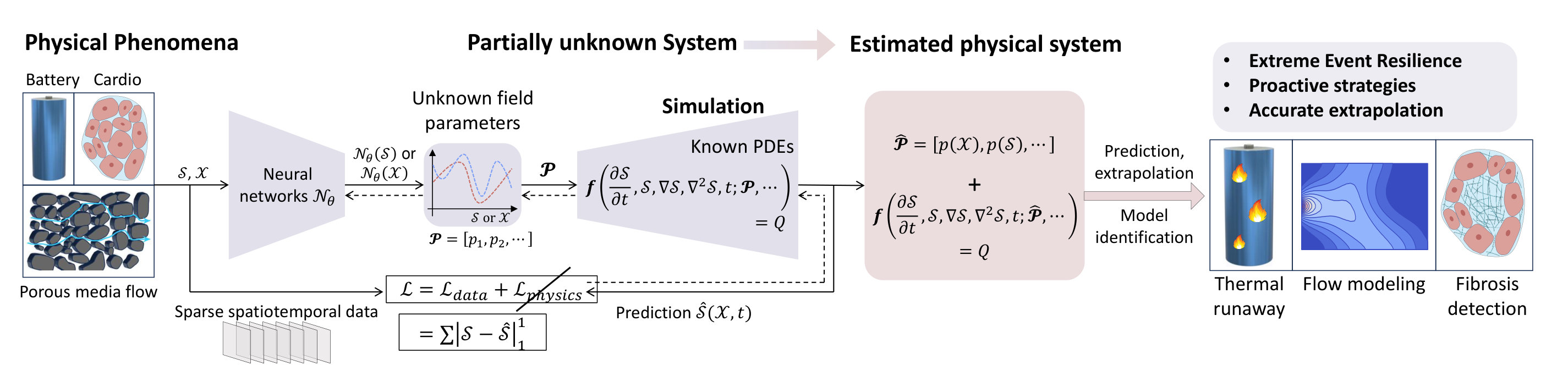 Figure 1
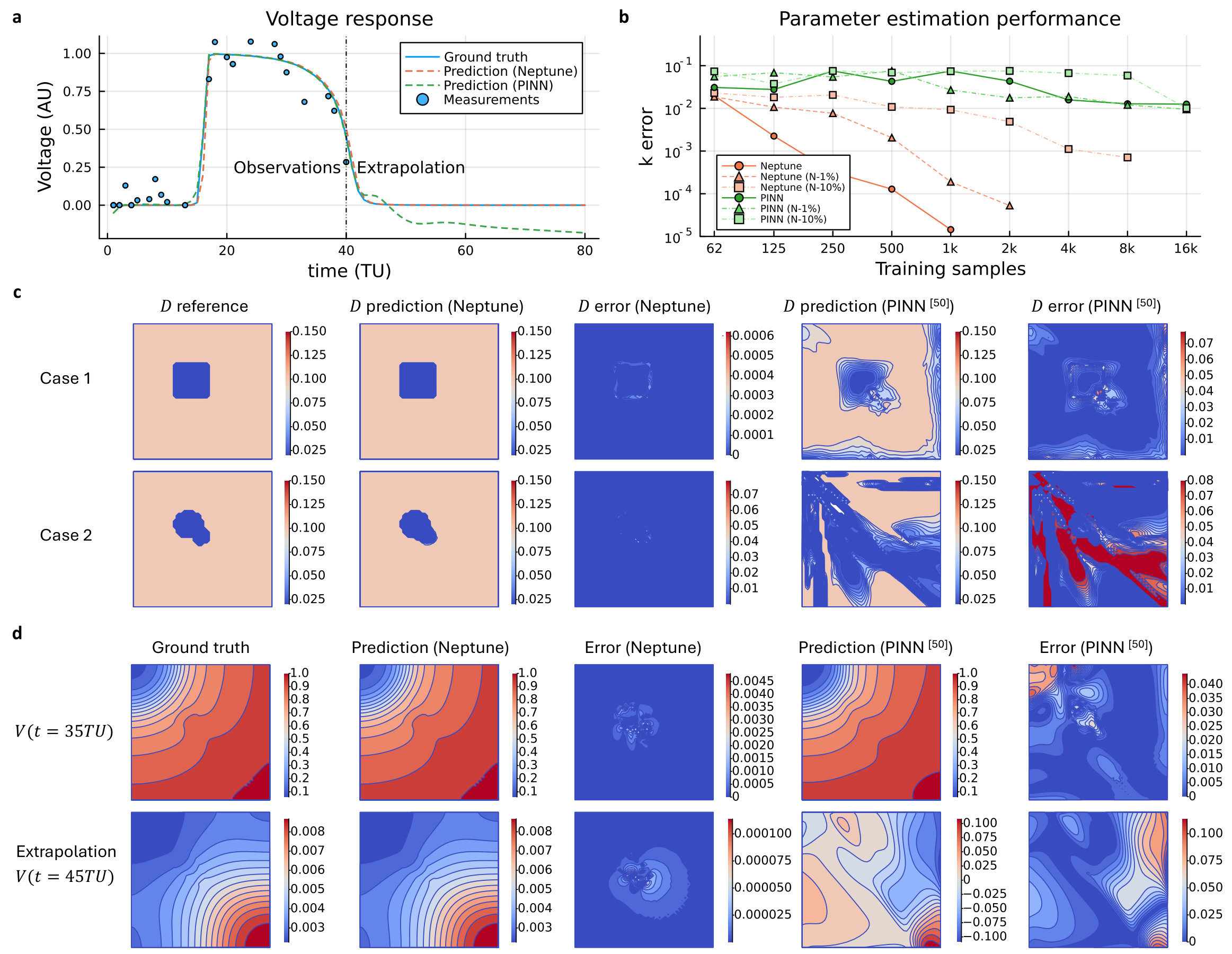 Figure 2
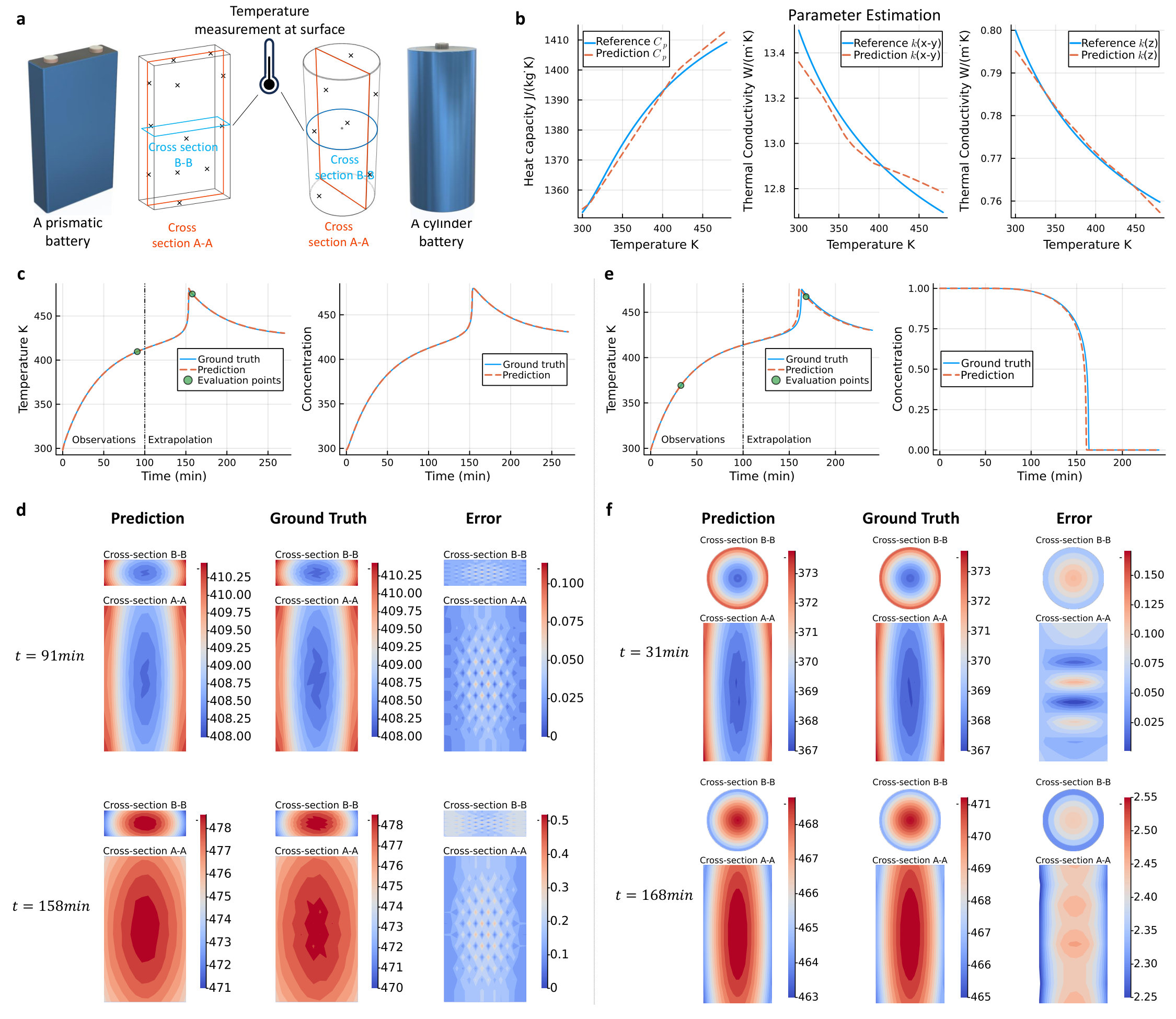 Figure 3
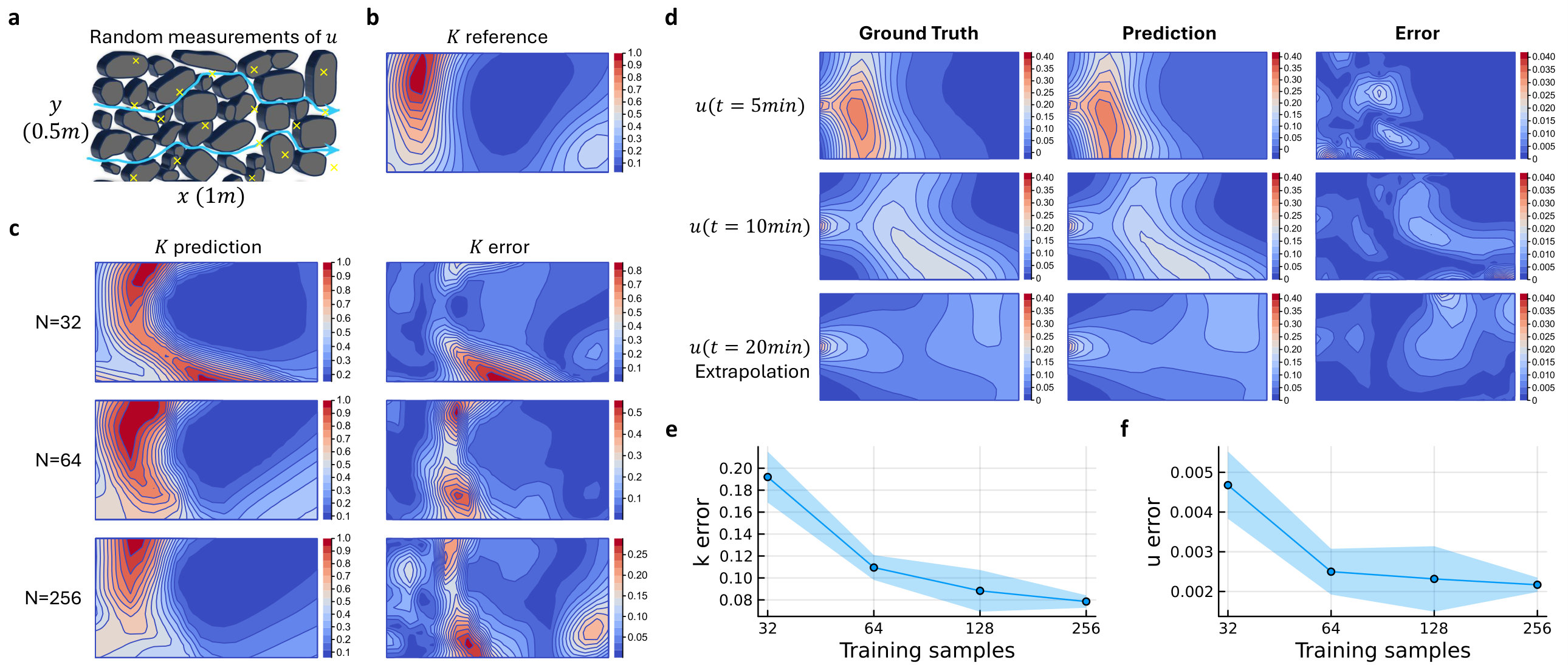 Figure 4
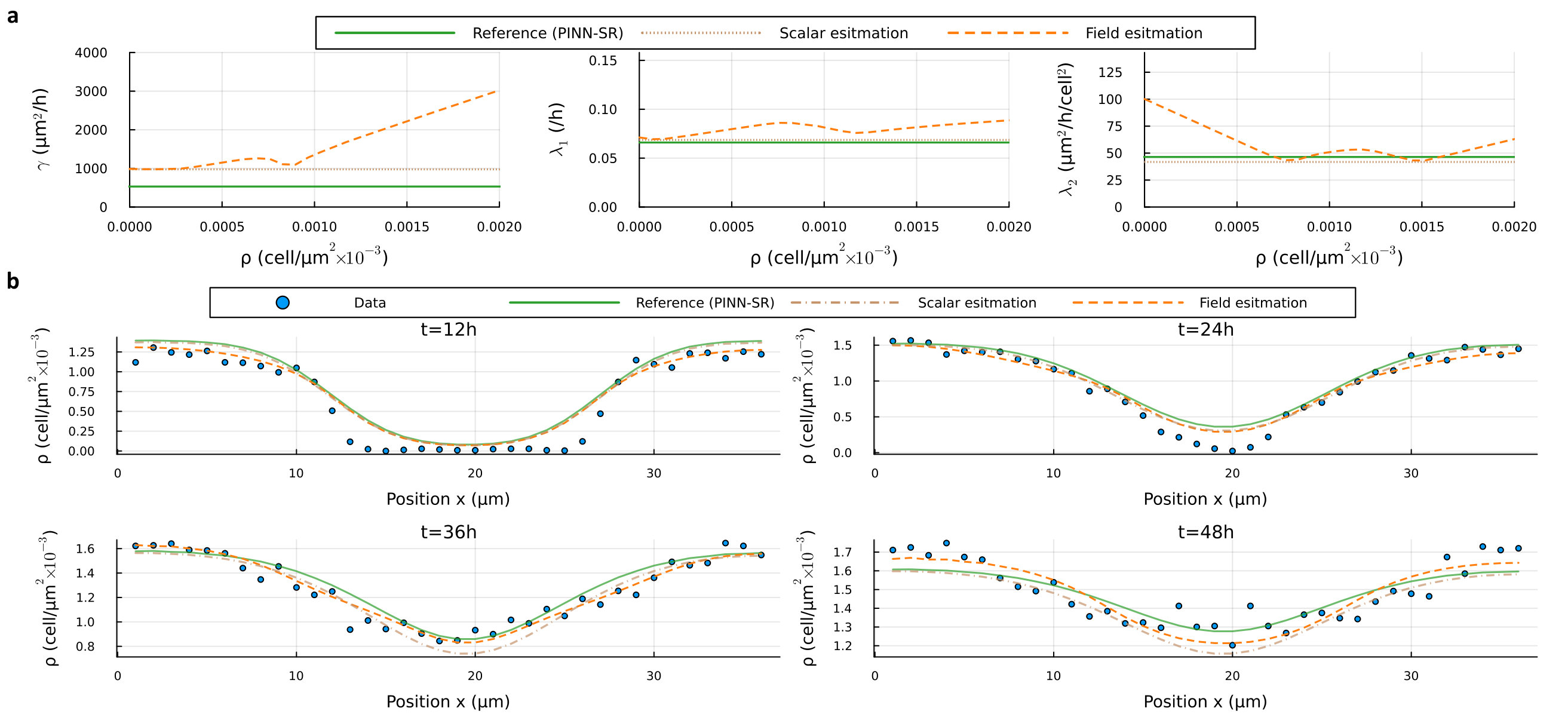 Figure 5
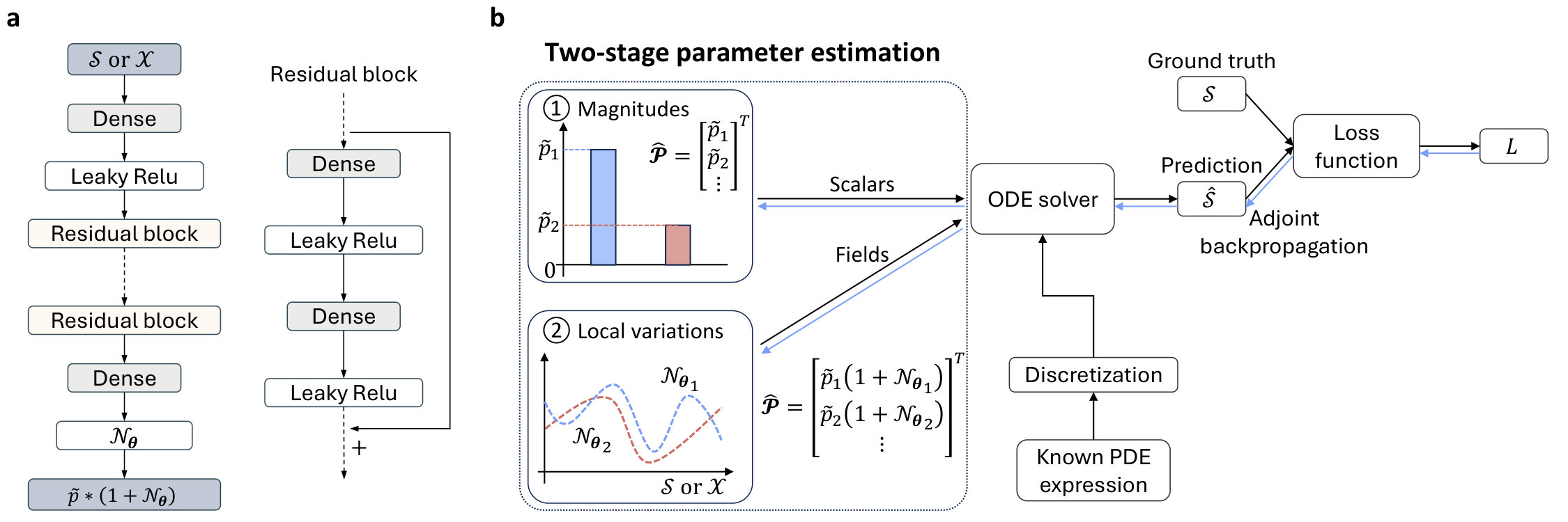 Figure 6
 Figure 7
| Application | Physics | Parameters | Measurements | Parameter | Extrapolated | |||||
|---|---|---|---|---|---|---|---|---|---|---|
| Error | Response Error | |||||||||
| Battery | Thermal & chemical | (conduct.), (heat cap.) | (temperature) | 0.81%, 1.23% | 0.36% | |||||
| Porous Flow | Darcy & dispersion | (hydraulic conduct.) | (concentration) | 8.83% | 0.69% | |||||
| Cardiac Electro | Aliev-Panfilov | (tissue conduct.) | (voltage) | 3.01% | 0.46% | |||||
| Cell Migration | Diffusion-reaction | (diffusion), (growth) | (density) | - | 6.40% |
Peer Reviews
No public reviews on file for this paper yet. If you reviewed it on a platform where reviews are public (OpenReview, ICLR, NeurIPS, ICML), you can paste yours below so the community can read it here.
Videos
No videos yet. Explain this paper in a talk, walkthrough, or lecture? Add one.
Estimating Parameter Fields in Multi-Physics PDEs from Scarce Measurements
Xuyang Li
Mahdi Masmoudi
Rami Gharbi
Nizar Lajnef
Vishnu Naresh Boddeti
Michigan State University, East Lansing, MI 48824, USA
Abstract
Parameterized partial differential equations (PDEs) underpin the mathematical modeling of complex systems in diverse domains, including engineering, healthcare, and physics. A central challenge in using PDEs for real-world applications is to accurately infer the parameters, particularly when the parameters exhibit non-linear and spatiotemporal variations. Existing parameter estimation methods, such as sparse identification, physics-informed neural networks (PINNs), and neural operators, struggle in such cases, especially with nonlinear dynamics, multiphysics interactions, or limited observations of the system response. To address this, we introduce Neptune, a general-purpose method capable of inferring parameter fields from sparse measurements of system responses. Neptune employs independent coordinate neural networks to continuously represent each parameter field in physical space or in state variables. Across various physical and biomedical problems, where direct parameter measurements are prohibitively expensive or unattainable, Neptune significantly outperforms existing methods, achieving robust parameter estimation from as few as 45 measurements, reducing parameter estimation errors by two orders of magnitude and dynamic response prediction errors by a factor of ten to baselines methods. More importantly, it exhibits superior physical extrapolation capabilities, enabling reliable predictions in regimes far beyond the training data. By facilitating data-efficient parameter inference, Neptune promises broad transformative impacts in engineering, healthcare, and beyond.
Accurate modeling of physical phenomena is crucial in a wide range of scientific and engineering applications. Differential equations provide a foundational framework for capturing dynamics that evolve over time and space. However, the governing parameters are often unknown or deviate from known values due to factors such as aging, wear, or environmental variation, resulting in significant changes in system behavior. For example, the thermal properties of aged batteries can evolve, increasing the risk of thermal runaway and fires in electric vehicles (EVs). Similarly, in biomedical contexts, changes in cardiac tissue properties can lead to arrhythmias or atrial fibrillation, while variations in porous media flow properties may cause groundwater contamination or aquifer depletion. These examples underscore the critical need for parameter estimation, as failing to account for evolving parameters can lead to inaccurate predictions and severe consequences. Beyond accuracy, parameter estimation enables transformative applications, such as simulating future behavior, predicting failure points, estimating remaining useful life in engineering systems, and creating personalized models for tailored healthcare diagnostics and treatments through high-fidelity digital twins.
Parameter estimation in multiphysics applications presents several interconnected challenges. The problem is ill-posed due to its inverse nature. In many real-world scenarios, direct parameter measurement is impractical due to cost, inaccessibility, or physical constraints, leaving system responses as the only observable data. In addition, available system response data are often sparse, noisy, or incomplete, limiting reliable parameter recovery. More critically, many relevant parameters are not scalar but spatially distributed or field-dependent, and are often tightly coupled across scales, making them difficult to isolate or model independently.
Despite notable progress in parameter estimation methods, significant limitations remain, particularly when addressing nonlinear multiphysics systems or time-dependent behaviors. Traditional approaches such as finite element updating [1, 2, 3], Bayesian neural networks [4], least squares estimation [5, 6], Kalman filtering [7, 8], Gaussian processes [9, 10, 11], and sparse identification [12, 13] are effective in simplified, single-physics problems. However, they struggle with spatially and temporally varying parameters in nonlinear multiphysics systems. Karhunen–Loève expansions [14, 15, 16] can represent parameter fields, but have limited applicability to time-dependent processes [14, 15, 17] and often require prior assumptions about parameter distributions [16].
Recent machine learning based approaches, such as PINNs [18, 19, 20, 21, 22, 23, 24, 25, 26, 27, 28, 29, 30, 31, 32], Neural Operators [33, 34, 35, 36, 37, 38, 39, 40, 41], and other deep surrogates [42, 43, 44] have emerged as efficient alternatives for modeling complex, field-dependent parametric systems. However, growing evidence [45] shows that these methods often rely on weak numerical baselines and suffer from reporting biases, leading to overoptimistic claims of performance and generalization. PINNs embed governing equations into neural network loss functions, enabling simultaneous learning of system dynamics and parameter fields [46, 47, 48, 49, 20, 50]. While effective in simple cases, PINNs struggle to train or recover complex parameters from extremely sparse or noisy data, particularly in nonlinear, coupled multiphysics systems, due to the dual objectives of simultaneous forward and inverse modeling [51, 17, 52, 53, 54]. PINN-SR [13], which incorporates sparse regression principles (SINDy) [12] for parameter and equation discovery, faces challenges in generalizing to systems with parameter fields. Neural Operators, such as DeepONet [33] and Fourier Neural Operators (FNO) [34], learn solution maps directly from data and have been extended to inverse problems [55, 56, 57, 58], yet often require large, high-fidelity datasets comprising thousands of samples [59, 60] and are sensitive to training data distribution [61] and hyperparameter choices [40, 61, 59].
A separate line of work builds on the differential equation framework by embedding neural networks into the governing dynamics, as in neural ODEs [62, 63, 64, 65, 66, 67] and universal differential equations [68]. Coupled with adjoint methods [68, 63], they enable memory‑efficient parameter estimation. Yet the majority of existing work targets low‑dimensional ODEs with scalar parameters and known equations, without extending to PDE‑governed systems or spatially/temporally varying parameter fields [69, 70, 71, 72]. One underlying reason is the high dimensionality and ill‑posedness of field estimation, where directly optimizing all local parameters leads to an enormous search space and unstable convergence. These challenges highlight the need for structured estimation strategies that can first capture dominant system behavior, before resolving more localized variations.
To address these limitations, this article introduces Neptune (Neural Estimation of Parameters in mulTi-physics PDEs Under sparse obSErvations), a generalizable and robust method for parameter field estimation in complex systems (see Figure 1). Neptune extends the universal differential equations framework from simple ODEs to multiphysics and coupled PDEs using finite difference discretization, while remaining compatible with standard numerical solvers. Neptune still utilizes adjoints for optimization, but it combines known governing equations with coordinate neural networks to infer unknown parameter fields, and requires no assumptions about their prior distributions. A core feature of Neptune is a structured two-stage estimation strategy: first recovering coarse scalar parameters, then refining spatially-varying fields via neural networks. This enables scalable recovery of multiple, high-resolution parameter fields in coupled systems.
Neptune inherits the flexibility of standard numerical solvers by discretizing governing PDEs into ODE systems via finite differences, enabling direct integration into existing simulation workflows. It does not rely on any prior assumptions about parameter distributions, and remains robust across a wide range of nonlinear, coupled multiphysics systems. By solving directly from the governing equations, Neptune demonstrates strong generalization and extrapolation capabilities, delivering accurate predictions beyond the training region and across diverse physical domains. These properties allow Neptune to achieve accurate and data-efficient parameter estimation, even under extremely sparse and noisy observations. Our key contributions are as follows:
- •
Generalizable framework for multiphysics PDEs. Neptune extends universal differential equations to high-dimensional, coupled systems, without requiring prior assumptions on parameter distributions.
- •
Two-stage parameter field estimation. A coarse-to-fine strategy enables scalable recovery of complex, spatially-varying parameter fields.
- •
Strong generalization from physics priors. Leveraging known governing equations, Neptune extrapolates reliably beyond training regions and under sparse observations.
In the following sections, we demonstrate Neptune’s versatility and efficacy across various scientific domains, including cardiac modeling, thermal-chemical battery systems, porous media flow, and cell migration. These applications showcase Neptune’s robustness under scarce and noisy data, adaptability to complex real-world settings, and strong predictive accuracy. Quantitative results in Tables 1 and 2 highlight Neptune’s consistent performance in parameter estimation across tasks.
I Cardiac Electrophysiology
Cardiac electrophysiology (EP) [73, 74, 75, 51] emphasizes the crucial coupling between cardiac tissue properties and the generation as well as propagation of electrical signals within the heart.
Known Physics: The canine ventricular Aliev-Panfilov model is utilized in this section, with the coupled equations [51] defined in the following.
[TABLE]
This model is commonly used to identify tissue heterogeneities, particularly from in silico data [76, 77, 51], with significant clinical potential for detecting fibrosis and other localized pathologies linked to arrhythmias and atrial fibrillation [51, 77]. The diffusion tensor , the target parameter, determines propagation speed, with as the measurable voltage and as an intermediate state variable. The PDEs describe the evolution of electrical potential and ionic currents in cardiac tissue, incorporating known properties such as tissue conductivity and reaction-diffusion dynamics.
Unknown Parameters: The key parameter, tissue conductivity (proportional to the diffusion tensor ), varies spatially and is challenging to measure directly, requiring estimation for accurate modeling. For simplicity, the estimation focuses on . Details of all known physical parameters and conditions relevant to this problem, along with those for other cases discussed in the article, can be found in Supplementary Note 1.
Problem Setup: A 2D slab of cardiac tissue is employed () as the spatial domain and aims to recover the heterogeneous diffusion parameter . Healthy tissue is represented by , while fibrosis tissue has five times smaller. is approximately [51]. During training, Gaussian noise is added to the training data ( measurements) to mimic real-world situations. The voltage response over time (from 0 to 40 ) at a randomly selected spatial point, including noise, is shown in Fig. 2a.
Measurements (with details and comparison to baselines): Neptune demonstrates exceptional efficiency and precision in joint parameter estimation and dynamic prediction. It achieves highly accurate and stable parameter estimates with as few as 1,000 measurements, maintaining robust performance even when utilizing only 62 sparse measurements on a mesh. Furthermore, Neptune significantly outperforms alternative approaches under noisy conditions, demonstrating superior accuracy and stability under challenging, data-limited scenarios. In contrast, the PINN model [51] requires a substantially higher data density to achieve functional results, needing at least 8,000 spatiotemporal measurements on a much finer mesh. As illustrated in Figure 2b, PINN consistently exhibits higher estimation errors across all data scales. Beyond estimation accuracy, Neptune maintains physical consistency during temporal extrapolation, whereas PINN tends to generate predictions that violate underlying physiological laws (Figure 2d). Finally, the FNO model was validated on a grid over 3 total time steps, totaling 2,700 measurements. While FNO provides a standard operator-learning benchmark, Neptune demonstrates a superior ability to recover parameters from significantly sparser and noisier measurement sets, as evidenced by the error plots in Figure 2c.
Analysis: Figure 2c evaluates the parameter estimation performance of Neptune, PINN, and FNO across two cases with distinct parameter distributions. The first column displays the reference distributions used as ground truth. In the second column, Neptune successfully recovers the parameters in both cases with high fidelity, achieving a Mean Absolute Error (MAE) of in Case 1 and in Case 2. By contrast, the FNO baseline performs reliably only in Case 1 (MAE: ), where the geometry aligns with its training distribution of rectangles, triangles, and circles. Case 2 reveals a clear sensitivity to out-of-distribution morphologies; while the FNO correctly identifies the spatial position of the target, it erroneously predicts a shape resembling a training circle rather than the actual underlying geometry, resulting in an increased MAE of . In the fourth column, PINN struggles significantly despite utilizing 50 times more data (50,000 vs. 1,000 measurements). In Case 1, PINN yields an MAE of which is about three orders of magnitude larger than Neptune and performs poorly overall. In Case 2, it fails to capture the random distribution of entirely, with the error further degrading to .
Figure 2d compares state variable predictions for Case 1 between Neptune and PINN. We note that FNO is excluded from this comparison because it cannot perform state variable predictions; unlike the physics-informed frameworks, FNO is trained as an end-to-end black-box estimator where the state variable serves as the input to predict the parameter. Furthermore, FNO is strictly constrained to structured grid data representations, whereas Neptune and PINN utilize flexible pointwise measurements.While PINN performs reasonably well within the training region (Fig. 2d, first row), its peak error remains an order of magnitude higher than that of Neptune. For temporal extrapolation (second row), PINN exhibits significantly larger errors due to its inaccurate estimation of . As shown in Fig. 2a, Neptune consistently adheres to the underlying physics, providing robust predictions even beyond the training window. It achieves accurate temporal extrapolations beyond 40 with an MAE of 0.00035 which is over two orders of magnitude lower than the PINN MAE of 0.066. Moreover, PINN frequently predicts non-physical negative values at multiple timesteps, further highlighting its limitations. A comprehensive analysis of these methodological differences and additional results under extremely sparse measurement conditions are provided in Supplementary Note 2 and 2.2.
Implications: The ability of Neptune to accurately estimate spatially heterogeneous parameters and predict state variables even under sparse, noisy conditions showcases its superiority over traditional methods like PINN. This advancement holds great promise for improving the diagnosis and modeling of cardiac pathologies, such as fibrosis and arrhythmias, where tissue heterogeneities play a critical role in understanding electrical signal propagation.
II Thermal Runaway in Batteries
Modern lithium-ion batteries are designed to achieve high energy density, extended operational durations, and rapid charging capabilities, catering to the power requirements of contemporary electric vehicles (EVs). These high-performance batteries provide substantial benefits but also pose safety challenges, particularly the risk of thermal runaway (TR), which in extreme cases can result in fire accidents [78]. To address these risks, a thorough understanding of the underlying physics is crucial.
Known Physics: TR is often governed by well-established thermal reactions and chemical kinetics, which are mathematically described by the following equations.
[TABLE]
and represent the battery temperature and concentration of reacting materials. Other variables such as energy release , heat release , active material content , activation energy , gas constant , and porosity are described in more detail in Supplementary Note 1.
Unknown Parameters: The parameters of interest [79, 80, 81] are temperature-dependent heat capacity , thermal conductivity , and a scalar parameter called the pre-exponential factor . For prismatic batteries, thermal conductivity is divided into cross-plane () and in-plane () components, whereas for cylindrical batteries, it is characterized by radial and longitudinal components. The pre-exponential factor is specifically introduced to illustrate the generalizability of the method.
These parameters are difficult to measure directly and are expected to behave as field variables influenced by the battery’s internal states, such as temperature and other dynamically changing properties during operation. Additionally, properties like thermal conductivity and heat capacity can exhibit significant variability due to mass production inconsistencies and further evolve over their service life from aging effects [82] and environmental influences [83]. This variability makes these parameters difficult to measure directly, but essential for understanding battery performance and predicting the likelihood of TR incidents.
Problem Setup: A standard prismatic battery () and a cylindrical battery ( height, diameter) (see Fig. 3a) are modeled to simulate TR behavior [84]. The initial condition is room temperature, with constant heat convection as the boundary condition (BC), and high external heat applied to simulate overheating.
Measurements: Considering real-life constraints, only surface temperatures can be measured, and only at limited locations. For training, we take just three measurement locations, with 15 temporal measurements each, during the initial 100 minutes before the irreversible temperature rise at around 150 minutes in TR.
Analysis: Despite this limitation, Neptune accurately estimates the parameter fields (, and ). For the prismatic battery, the estimated parameters (Fig. 3b) show MAE of 1.88, 0.052, and 0.001, compared to reference values of 1400, 13, and 0.8, respectively. For the cylindrical battery, the scalar parameter is jointly estimated, with an estimated value of showing a low percentage error of 0.97% compared to the reference . Similar accuracy is achieved for other parameters, with results detailed in Supplementary Note 2. Furthermore, Neptune also demonstrates robustness under noisy measurements; for the prismatic battery, results for noise levels of 1% and 10% are detailed in Table 1.
Implications: Importantly, accurate parameter estimation enables the prediction of temperature changes of potentially ongoing TR. By integrating the parameters into the PDE system, predictions are extended over 0-270 minutes. Figure 3c shows the temporal predictions of average temperature and concentration () profiles, closely matching the ground truth. Besides, inner temperature distributions can also be evaluated. In Fig. 3d, representative results are displayed for cross-sections and (Fig. 3a) at two key stages, before and during TR, where temperature profiles are accurately predicted with minimal errors.
Additionally, accurate parameter estimation using Neptune enables model customization to simulate battery behavior under diverse initial and boundary conditions (illustrated in Supplementary Note 2). This capability supports predictive modeling for various scenarios, including environmental changes, manufacturing inconsistencies, and operational extremes, which are crucial for enhancing battery safety and performance. Unlike existing methods such as PINN, which often fail due to reliance on specific initial and boundary conditions, Neptune is independent of these constraints, ensuring consistent and reliable performance across scenarios. This robustness unlocks new opportunities for designing safer, more efficient batteries and evaluating their behavior over extended lifetimes or under extreme conditions.
III Flow in Porous Media
The flow of solutes in porous media is a fundamental phenomenon observed in various natural systems [85, 86, 87, 88, 89, 90, 91]. This includes critical environmental concerns such as contaminant transport in water and the greenhouse effect caused by carbon emissions.
Known Physics: As an illustrative example, we focus on subsurface transport, a problem frequently studied in recent literature [92, 17, 53]. This process is governed by coupled PDEs: the time-dependent advection-dispersion equation (ADE) and Darcy’s law. These equations describe time-dependent transport behaviors and the physics of fluid flow in porous media, which are key to understanding and predicting such systems.
[TABLE]
where state variable represents the particle concentration field. Variables such as average pore velocity , dispersion coefficient , hydraulic head , and porosity are described in more detail in Supplementary Note 1.
Unknown Parameters: In this system, solute movement through porous media varies due to environmental conditions, human activities, and geological processes, making accurate parameter estimation of hydraulic conductivity crucial for understanding these phenomena and addressing these pressing issues [93, 17, 53, 94]. However, is often difficult to measure directly, whereas particle concentration fields, depending on the system and measurement tools, can be relatively easier to retrieve.
Problem Setup: A 2D computational domain of and is defined [92], as shown in Fig.4a. Using just 32 random spatial-temporal concentration measurements over 0–16 minutes, the parameter field can be robustly estimated. Since the right-hand side of equation 7 is 0, multiple solutions exist, so the estimated is normalized and compared to the normalized reference (see Fig. 4b).
Measurements: Figure 4c shows the normalized estimation for different sample sizes ( 32, 64, 256). With fewer samples, the data may not fully capture the response, leading to larger prediction errors. However, even with just 32 points, Neptune already captures the key features of the parameter’s distribution. Increasing the number of samples enhances the resolution of predictions and further reduces estimation errors.
Analysis: Figure 4d illustrates the evolution of predictions over time. The first and second rows show contour predictions during the training region (at minutes and minutes) with low error and strong alignment with the ground truth. Notably, temporal extrapolation up to 20 minutes, beyond the 16-minute training region, accurately captures the concentration , as shown in the third row of Fig. 4d.
To demonstrate the robustness of Neptune, parameter estimation is repeated with varying sample sizes. Figure 4e shows the parameter estimation performance, while Fig. 4f displays the corresponding response prediction accuracy, with errors significantly reduced at 64 samples. Ablation studies on neural network sizes, detailed in Supplementary Note 4, further validate the model’s robustness and generalizability. For comparison with PINN-based approaches, we implemented state-of-the-art training techniques following recent best practices: residual-based adaptive sampling [95, 96] to dynamically refine collocation points in high-residual regions, 64-bit floating-point precision [97] to improve numerical stability, balanced residual decay rate (BRDR) loss weighting [98] to ensure balanced convergence across loss components, and a multi-phase training strategy with second-order optimization [24, 99] using L-BFGS-B for fine-tuning. The PINN implementation details and comparison results are provided in Supplementary Note 2.3. Additionally, a spline-based parameter fitting method was tested as a non-neural network strategy but showed lower performance than Neptune (around 2 times larger mean errors in both the parameter estimation and response prediction). The spline-based parameter fitting setups and results can be found in Supplementary Note 6.
Implications: Accurately estimating the hydraulic conductivity field and predicting solute transport dynamics with Neptune enables robust modeling of subsurface transport, even with sparse and noisy measurements. This capability is critical for addressing environmental challenges such as contaminant transport and groundwater management, where accurate parameter estimation and temporal predictions are essential for effective decision-making.
IV Cell Migration and Proliferation
Application and Known Physics: This section presents an experimental study of the diffusion (cell migration) and reaction (cell proliferation) process, which is governed by a known form of PDE [102, 103, 13].
[TABLE]
where parameters such as cell diffusivity and proliferation rates and define the characteristics of cell migration and proliferation.
Unknown Parameters: These parameters are unknown and require estimation from cell density observations. According to the Porous-Fisher model [100, 101], cell diffusivity varies with density (Fig. 5b), increasing with higher cell density, while proliferation rates and are treated as constants. However, to demonstrate Neptune’s generalizability, all 3 parameters are modeled as density-dependent fields.
Problem Setup: The experimental data were originally extracted from high-resolution imaging collected in previous research on in vitro cell migration (scratch) assays [104], and were further analyzed [13] aimed at discovering the governing equation. The preprocessed data describes the cell density distributions at 38 evenly distributed spatial points in one dimension and only at 5 time steps (). The spatial domain ranges from 0 to 1900 . A detailed description of the experiment setup and data preprocessing can be found in the previous research [104, 13]. This spatial-temporal experimental data is extremely sparse and noisy.
Measurements: Given the initial condition at 38 points from the experimental data () and Neumann boundary conditions and , we train Neptune with only 152 cell density data points over 38 spatial points and 4 timesteps. In the same setup, we compared our Neptune with PINN-SR [13] (i.e., PINN with sparse regression), for parameter estimation and response prediction performance.
Analysis: As shown in the first graph of Fig. 5a, Neptune estimates an increasing with cell density, consistent with previous research [102, 103]. Field estimations also suggest and are likely scalars. We also assume space-dependent parameters for estimation: results showing parameter distributions with high (peak) values at two boundaries, demonstrating that the parameter fields are density (or state) dependent. In the third graph, while the field estimation for shows large values at low densities and stabilizes as density increases, this behavior is primarily due to highly noisy experimental data in regions with low cell numbers, rather than being attributed to the nature of the parameter field itself. In contrast, PINN-SR, limited by its methodology, cannot estimate parameter fields, and its scalar estimations show slightly different combinations but remain within a reasonable range. This limitation is evident at (first graph) and (last graph), where it fails to capture enhanced cell spreading.
Accurate parameter field estimation excels in predicting cell density distributions over time, as shown in Fig. 5b. For such sparse and noisy data, PINN-SR achieves a median error of . In contrast, Neptune, assuming density-dependent parameters, achieves the highest accuracy with an error of . Across experimental data with varying initial cell densities [13], Neptune achieves 28-47% lower median errors. Additional results are detailed in Supplementary Note 2.
Implications: The findings demonstrate that Neptune not only provides more accurate parameter estimations under sparse and noisy conditions but also captures critical density-dependent dynamics that other methods, like PINN-SR, cannot. This capability enables improved predictions of biological phenomena such as cell migration and proliferation, offering new avenues for understanding and modeling reaction-diffusion systems in complex and noisy experimental scenarios.
V Discussion
In this paper, we presented Neptune for accurate parameter field estimation under scarce observation data, demonstrated by various PDE problems in emerging fields where physical parameters are unknown and important. Specifically, we estimated the thermal conductivity and heat capacity in coupled thermal problems, enabling accurate TR prediction. In porous media flow, spatially varying hydraulic conductivity was recovered, improving the modeling of phenomena such as contaminant transport. For cardiac EP, tissue electrical conductivity was inferred solely from voltage measurements, offering potential for detecting fibrosis and other localized pathologies. Finally, the cell migration and proliferation case demonstrates effective parameter estimation under real-world noisy and sparse data conditions. It also highlights the method’s capability in discovering governing equations and its generalizability in estimating scalar variables.
In terms of utility, Neptune demonstrates its generalizability and robustness to estimate multiple parameters simultaneously across various dependencies (spatial, state, and even time), each exhibits distinct patterns. The proposed two-stage learning strategy further enhances effectiveness by handling parameters across different scales. By first estimating scalar magnitudes, it significantly reduces the search space, allowing neural networks to focus on learning local variations within the parameter field. Furthermore, we extend this discussion to demonstrate the superior performance of our strategy compared to other training approaches, including: (1) estimating only scalars, (2) directly estimating each parameter field in one step using separate neural networks; (3) estimating all parameter fields within a single neural network; and (4) jointly estimating scalar magnitudes and field variations in a single step. Detailed comparisons are provided in Supplementary Note 5. Compared to other fitting methods, Neptune significantly outperforms spline-based approaches in capturing complex parameter distributions. In addition, the use of FDM makes the method easily adaptable to a wide range of PDEs. While less effective for handling shock waves or large discontinuities, it offers favorable computational efficiency and supports gradient-based optimization.
Compared to sparse identification methods like PINN-SR, Neptune models full parameter field distributions rather than scalars, achieving 27–47% improvement in forward response accuracy. This methodological shift enables more detailed modeling of the underlying physical processes, leading to improved predictive accuracy. Additionally, compared to PINN, our framework offers stronger temporal extrapolation, better adherence to physical laws, and greater adaptability to boundary and initial condition changes. It also requires less data, making it ideal when measurements are limited or costly. However, inverse problems like parameter estimation remain ill-posed and prone to local minima, especially with complex fields or limited data. These challenges can be mitigated by using informed initial guesses and incorporating prior knowledge, such as parameter magnitudes, smoothness penalties, and strategic data selection. Future work may extend the method to more general finite element frameworks and explore its application to modeling and parameter estimation in chaotic systems.
VI Methods
Problem Setup and differentiable PDE solver We consider a general time-dependent PDE of the form encompassing a range of PDE-governed systems studied in this work:
[TABLE]
where is the state variable defined over spatial domain (e.g., , , or ) and time interval . The unknown parameters represent latent or field-dependent quantities of interest. The terms and denote the spatial gradient and Laplacian of the state variable, respectively. Neptune directly solves PDE systems by applying FDM for spatial discretization and using differentiable ODE solvers for time integration. This approach ensures efficient and accurate forward simulations while enabling gradient computation through the solver via the adjoint method, significantly enhancing training speed. Using evenly spaced mesh nodes, the second derivative in the -direction at a point is approximated by the central difference scheme [105]:
[TABLE]
where is the mesh spacing and is the discrete state value at . The term denotes the truncation error, indicating second-order spatial accuracy.
In most scenarios considered in this study, the spatial dimensions of the state variables are organized into a 1D vector form for computational efficiency. The state variable and discretization matrices are structured as and , where denotes the total number of spatial nodes in the discretized 3D domain. Spatial derivatives of various orders are explicitly formulated for each direction, as shown in equation 12:
[TABLE]
where represents the derivative order and the matrix numerically approximates the corresponding spatial derivative.
Substituting the finite difference discretizations into the general PDE form yields the semi-discrete system:
[TABLE]
where and denote the numerical approximations of the first- and second-order spatial derivatives, respectively. Boundary conditions are carefully handled during discretization. Two types, Dirichlet and Neumann, are considered, expressed as or , where is the prescribed coefficient. Boundary conditions are implemented by modifying the discretization matrices in equation 12, following standard approaches [106, 107]. After discretization, the PDE system is reformulated as a set of ODEs and solved using Runge–Kutta methods [108], with dynamics extracted at observation times.
Parameter field modeling with neural networks Neptune models the unknown parameter field as:
[TABLE]
where denotes a learnable scalar and represents the neural network with layers and learnable weights as . A detailed architecture with skip connections can be referred to Fig. 6. denotes a neural layer and represents function composition. The input to can be discretized values of space or state , and are properly scaled (i.e., -1 to 1 from or observed ). Leaky ReLU activation functions are used in all layers except the final one, which omits activation functions. For multiple parameter fields , Neptune simply employs different scalars and networks for parallel modeling, where
Two-stage parameter estimation strategy Neptune employs a two-stage learning, first optimizing and then training . In the first stage (see the upper row of Fig. 6), random scalars are initialized and incorporated into the discretized governing equations to numerically solve for the dynamic response . This is equivalent to setting in equation 14. Those learnable scalars are optimized using the adjoint method [62] (detailed later in the section) by minimizing the error between and the observed measurements . The second stage fixes the converged scalars and only optimizes the neural network weights , aiming to estimate local variations in a reduced search domain (see the lower row of Fig. 6).
During the optimization, scalars act as a physics-based prior and implicit regularizer, ensuring early physical stability of training and providing a well-scaled baseline for convenient expansion to parameter fields in the second stage. Even if converges with high error, its combination with the PDE remains physically meaningful and stable during optimization.
In the second stage, the neural network acts primarily as a correction term, analogous to residual learning architectures such as ResNet [109]. Initially, the fixed scalar constrains the neural network to explore only perturbations around a physically meaningful baseline. This constraint stabilizes gradient flow, prevents nonphysical field magnitudes, preserves the well-posedness of the underlying PDE, and generally improves training stability. Meanwhile, in later stages of training, the neural network is allowed unbounded exploration (in most cases, no activation is applied to the final layer), enabling it to capture more complex behaviors beyond the initial physics-based prior.
Compared to directly learning with a neural network, the first-stage scalar learning significantly accelerates training, as numerically solving the PDE with parameter field modeling is several times more expensive, depending on model complexity. It also reduces the search space and greatly stabilizes the second-stage learning of .
In addition, by anchoring the field prediction around a physically meaningful baseline, this strategy improves generalization and robustness during training. The gradient flow with respect to inherits better conditioning from the scalar optimization step, further enhancing convergence efficiency and training stability. Mathematically, the gradient with respect to the scalar parameter in the first stage is given by
[TABLE]
where because in state one.
In the second stage, following the reparameterization in equation 14, the gradient with respect to the network parameters becomes
[TABLE]
Thus, the core physical gradient is consistently inherited across both stages, ensuring smooth convergence and stable optimization dynamics.
Neural network architecture and problem-specific design The coordinate neural networks (feed-forward) in the second stage are adaptively designed, with the number of residual blocks and neurons per layer customized for each application. Specifically, in the thermal battery problem, the scalar references for thermal conductivity in different directions (, ) and heat capacity () are first determined. In the cell migration problem, three scalar parameters, , , and , are similarly estimated. In both cases, the neural network models state-dependent parameter fields based on a single state variable, with a network input size of 1 (e.g., temperature or density , rescaled approximately from -1 to 1). A compact network with 20 neurons per hidden layer and two residual blocks is used to ensure efficient training.
In contrast, for the flow and cardiac applications, the conductivity parameters or depend on a 2D space, requiring larger neural networks: 50 neurons with 3 residual blocks for the flow problem, and 150 neurons with 4 blocks for the cardiac problem. The spatial inputs (, ) are rescaled from to in both dimensions. Notably, in the flow problem, multiple parameter distributions can satisfy the same setup due to the nature of equation 7, which involves taking spatial derivatives. Therefore, the first-stage scalar estimation is omitted, and the neural network is directly trained to predict relative variations by outputting . An absolute value activation with a small offset is applied at the final layer to ensure strictly positive predictions and avoid physically meaningless zeros.
Additionally, Supplementary Note 4 presents an ablation study evaluating the impact of neural network size on parameter estimation performance, while Supplementary Note 5 provides a detailed comparison of this training strategy against alternatives, including direct parameter field learning and using a single neural network for all parameters.
Loss function and model training Neptune relies solely on observations from physical phenomena for training. The loss function is defined purely using the mean absolute error (MAE):
[TABLE]
where and represent the ground truth (observations) and predicted responses, respectively, is the number of points. Preliminary experiments showed that mean squared error (MSE) yielded similar performance, and thus, MAE was chosen for simplicity. Regularization terms (e.g., weight decay) were also tested but adversely affected optimization and were therefore omitted.
During training, observations are split into mini-batches of size 16 (reduced to 8 for the cell migration problem due to limited samples). In the first stage, the loss is minimized to directly learn , with the learning rate adaptively decreasing from 1 to until convergence, where stabilizes without further change. Dashed lines in the figure illustrate the gradient flow during optimization. In the second stage, the loss is minimized to optimize the neural network weights , with a smaller learning rate ranging from to depending on network size. The best-performing , corresponding to the lowest loss value, is saved as the final trained model. The parameter field is then predicted using equation 14 with the corresponding spatial or state inputs.
To update the learnable weights ( or ), Neptune employs gradient-based optimization through adjoint sensitivity analysis [62], leveraging advancements in neural ODEs and reverse-mode automatic differentiation [68, 63]. For the scalar parameters , the adjoint method directly computes the loss gradient through the PDE solver, as shown in equation 16. For the neural network weights , an additional application of the chain rule through the neural network is required, as detailed in equation 17.
Importantly, Neptune differs fundamentally from traditional neural ODE approaches: instead of modeling unknown or partially known governing expressions with neural networks, it tackles complex PDEs with fully known equations, while neural networks serve only as correction terms for modeling unknown parameter fields. To clarify the underlying optimization, we next emphasize the derivation of the common term for a standard differential equation. The adjoint method requires defining a scalar functional , where is the numerical solution to the differential equation with and initial condition . In our experiments, we assume a known initial condition.
In our work, though the PDE system is discretized spatially using equation 13, this semi-discretization does not fundamentally alter the adjoint sensitivity formulation. Adjoint sensitivity analysis is still applied to compute the gradient of with respect to the parameters :
[TABLE]
To derive the adjoint equation [110], we introduce the Lagrange multiplier to form:
[TABLE]
Since , we have that:
[TABLE]
where represents the sensitivity of the state variables to the parameters. After applying integration by parts to the term involving , we require that:
[TABLE]
where is the Jacobian of the system with respect to the state , and is the Jacobian with respect to the parameters. The solution to the adjoint problem provides the sensitivities through the integral:
[TABLE]
To compute the term , the adjoint problem is formulated and solved as an ODE system. This is achieved using a specialized sensitivity analysis framework [68], which provides a range of numerical methods tailored to different types of PDE systems.
How Neptune outperforms PINN in inverse parameter estimation tasks? Here we demonstrate why PINN-based inverse parameter estimation fails and how our adjoint-based method fundamentally differs in its approach. This analysis uses flow in porous media as a representative example, though the moving target problem arising from simultaneous updates of parameters and state variables is general and applicable to other inverse problems where parameters and state variables are coupled through PDE constraints.
In the PINN formulation for inverse problems, the total loss consists of several components: represents the PDE residual losses enforcing the governing equations; represent boundary condition losses (8 terms in total) enforcing Dirichlet and Neumann conditions on the domain boundaries. These boundary conditions are defined as follows: Hydraulic head (): (1) : Neumann flux (inflow); (2) : Dirichlet (fixed head); (3) : Neumann no-flux; (4) : Neumann no-flux. Concentration (): (5) : Dirichlet Gaussian injection ; (6) : Neumann no-flux; (7) : Neumann no-flux; (8) : Neumann no-flux. is the initial condition loss enforcing the state at ; and is the data mismatch term comparing predicted values to observational data. The total loss is a weighted sum:
[TABLE]
where are loss weights.
The inverse estimation of the parameter field faces a fundamental optimization challenge arising from the coupled nature of the PDE residuals. The parameter (represented by neural network weights ) is updated exclusively through the gradients of the PDE residuals, which are the only non-zero terms in . However, these same loss terms simultaneously update the state variables through their respective gradients . The coupling is evident from the residual dependency . This creates a moving target problem during optimization: at iteration , the parameter attempts to minimize the PDE residuals based on the current state , but these state variables are concurrently being updated to by the same residual terms. As a result, the optimization landscape for shifts with each update, preventing stable convergence to the true parameter values. In contrast to the PINN approach, Neptune circumvents this optimization conflict by decoupling parameter estimation from state variable learning. The forward problem is solved using a numerical solver, which enforces a deterministic relationship between the parameter and the state variable. Critically, during optimization, only the neural network weights are updated; the state variable is not a free optimization variable but is uniquely determined by through the differentiable PDE solver at each iteration. This direct, one-way coupling eliminates the moving target problem: at iteration , the parameter minimizes the loss based on , and the subsequent state is fully determined by the updated parameter, ensuring a stable optimization landscape that enables reliable convergence to the true parameter values.
Data generation For the cell migration and proliferation problem, experimental data are sourced from previous research [104]. For other data, we generate data by employing FDM to solve the PDEs in each problem. For battery thermal runaway modeling, the mesh size is set to in each spatial dimension, with a timestep of (i.e., minutes over steps). The two state variables, temperature and concentration , are updated simultaneously at each step, along with the temperature-dependent parameters. Secondly, in the flow problem, the PDEs are solved in multiple stages. The mesh size is set to , and a reference parameter , based on previous research [17], is regenerated. The hydraulic head is computed using Darcy’s law (equation 7), followed by the velocity fields in the and directions, solved using and (equation 8). The resulting velocity field is then used to solve the time-dependent concentration equation for (equation 6). Thirdly, in the cardiac electrophysiology problem, the mesh size is set to in both and dimensions. The two state variables, and , are computed at each timestep (1) during the simulation. Lastly, in the cell migration and proliferation problem, the mesh size is fixed at points, corresponding to the spatial measurement positions. Due to varying gaps between the first two and the last two points, the standard FDM is modified to accommodate a non-uniform finite difference mesh. There are timesteps: the first for setting initial conditions, and the remaining for training.
Notably, Supplementary Note 3 expands on the mathematical derivation of finite difference discretization [111, 112, 113], explains the treatment of non-uniform meshes at geometry boundaries for the cell migration and proliferation problem, and discusses limitations of FDM. The training data, consisting of only the state responses, is generated numerically using the PDE solver for the first three scenarios, with different levels of Gaussian noise added to ensure robustness (details in Supplementary Note 1).
Data availability All synthetic training data are generated on-the-fly by our provided scripts. The experimental cell migration data, originally published in [104], are also packaged within our code repository. Additional information can be found in the Code availability section.
Code availability The source code used to generate the results presented in this study is provided as supplementary file for the peer-review process. The main algorithm is implemented in Julia, while baseline methods including PINNs and neural operators are implemented in Python (PyTorch). Upon acceptance, the code will be hosted on a public GitHub repository.
Author contributions N.L. and V.B. supervised the study. X.L., N.L., and V.B. conceived the initial idea. X.L. and M.M. conducted the numerical experiments. X.L., M.M., N.L., and V.B. wrote the paper. X.L., M.M., and R.G. contributed to the supplementary.
Competing interests The authors declare no competing interests.
Correspondence and requests for materials should be addressed to [email protected] and [email protected].
The reference list from the paper itself. Each links out to its DOI / PubMed record.
- 1Steenackers and Guillaume [2006] G. Steenackers and P. Guillaume, Finite element model updating taking into account the uncertainty on the modal parameters estimates, Journal of Sound and vibration 296 , 919 (2006).
- 2Ebrahimian et al. [2017] H. Ebrahimian, R. Astroza, J. P. Conte, and R. A. de Callafon, Nonlinear finite element model updating for damage identification of civil structures using batch bayesian estimation, Mechanical Systems and Signal Processing 84 , 194 (2017).
- 3Xu and Darve [2020] K. Xu and E. Darve, Adcme: Learning spatially-varying physical fields using deep neural networks, ar Xiv preprint ar Xiv:2011.11955 (2020).
- 4Yang et al. [2021] L. Yang, X. Meng, and G. E. Karniadakis, B-pinns: Bayesian physics-informed neural networks for forward and inverse pde problems with noisy data, Journal of Computational Physics 425 , 109913 (2021).
- 5Ji et al. [2020] Y. Ji, X. Jiang, and L. Wan, Hierarchical least squares parameter estimation algorithm for two-input hammerstein finite impulse response systems, Journal of the Franklin Institute 357 , 5019 (2020).
- 6Li and Liu [2020] M. Li and X. Liu, Maximum likelihood least squares based iterative estimation for a class of bilinear systems using the data filtering technique, International Journal of Control, Automation and Systems 18 , 1581 (2020).
- 7Varshney et al. [2019] D. Varshney, M. Bhushan, and S. C. Patwardhan, State and parameter estimation using extended kitanidis kalman filter, Journal of Process Control 76 , 98 (2019).
- 8Hossain et al. [2022] M. Hossain, M. Haque, and M. T. Arif, Kalman filtering techniques for the online model parameters and state of charge estimation of the li-ion batteries: A comparative analysis, Journal of Energy Storage 51 , 104174 (2022).