Generative Latent Space Dynamics of Electron Density
Yuan Chiang, Youngsoo Choi, Daniel Osei-Kuffuor

TL;DR
This paper presents a novel generative framework combining autoencoders and diffusion models to predict the time evolution of electron densities from quantum simulations, enabling stable long-term predictions and statistical fidelity.
Contribution
It introduces a new deep learning approach that models electron density dynamics using latent space diffusion, improving long-horizon stability and statistical accuracy over previous methods.
Findings
Accurately predicts electron density trajectories in liquid lithium at 800 K.
Captures spatial correlations and statistical structure of densities.
Enables stable long-term quantum dynamic simulations.
Abstract
Modeling the time-dependent evolution of electron density is essential for understanding quantum mechanical behaviors of condensed matter and enabling predictive simulations in spectroscopy, photochemistry, and ultrafast science. Yet, while machine learning methods have advanced static density prediction, modeling its spatiotemporal dynamics remains largely unexplored. In this work, we introduce a generative framework that combines a 3D convolutional autoencoder with a latent diffusion model (LDM) to learn electron density trajectories from ab-initio molecular dynamics (AIMD) simulations. Our method encodes electron densities into a compact latent space and predicts their future states by sampling from the learned conditional distribution, enabling stable long-horizon rollouts without drift or collapse. To preserve statistical fidelity, we incorporate a scaled Jensen-Shannon divergence…
Click any figure to enlarge with its caption.
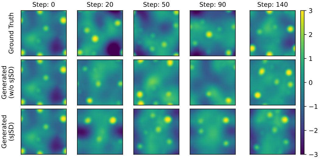 Figure 1
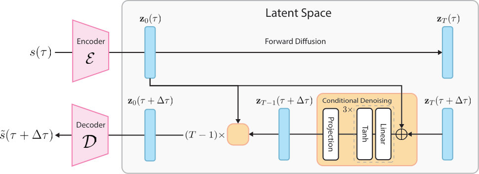 Figure 2
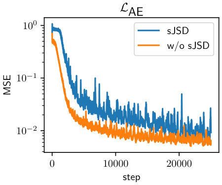 Figure 3
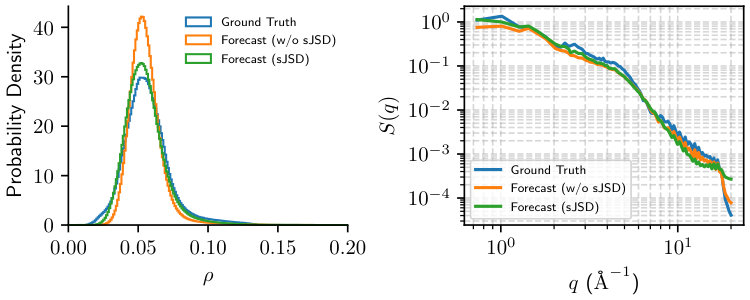 Figure 4
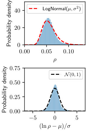 Figure 5
Peer Reviews
No public reviews on file for this paper yet. If you reviewed it on a platform where reviews are public (OpenReview, ICLR, NeurIPS, ICML), you can paste yours below so the community can read it here.
Videos
No videos yet. Explain this paper in a talk, walkthrough, or lecture? Add one.
Taxonomy
TopicsMachine Learning in Materials Science · Quantum, superfluid, helium dynamics · Quantum many-body systems
Generative Latent Space Dynamics of Electron Density
Yuan Chiang
University of California Berkeley
Lawrence Berkeley National Laboratory
&Youngsoo Choi
Center for Applied Scientific Computing
Lawrence Livermore National Laboratory
&Daniel Osei-Kuffuor
Center for Applied Scientific Computing
Lawrence Livermore National Laboratory
[email protected] work started as a student at Lawrence Livermore National Laboratory.
Abstract
Modeling the time-dependent evolution of electron density is essential for understanding quantum mechanical behaviors of condensed matter and enabling predictive simulations in spectroscopy, photochemistry, and ultrafast science. Yet, while machine learning methods have advanced static density prediction, modeling its spatiotemporal dynamics remains largely unexplored. In this work, we introduce a generative framework that combines a 3D convolutional autoencoder with a latent diffusion model (LDM) to learn electron density trajectories from ab-initio molecular dynamics (AIMD) simulations. Our method encodes electron densities into a compact latent space and predicts their future states by sampling from the learned conditional distribution, enabling stable long-horizon rollouts without drift or collapse. To preserve statistical fidelity, we incorporate a scaled Jensen-Shannon divergence regularization that aligns generated and reference density distributions. On AIMD trajectories of liquid lithium at 800 K, our model accurately captures both the spatial correlations and the log-normal-like statistical structure of the density. The proposed framework has the potential to accelerate the simulation of quantum dynamics and overcome key challenges faced by current spatiotemporal machine learning methods as surrogates of quantum mechanical simulators.
1 Introduction
The theoretical description of electrons and nuclei forms the cornerstone of understanding the physical and chemical properties of matter, yet it remains one of the most challenging frontiers of modern quantum mechanics. Electronic structure calculations, while offering a pathway to predict the ground and excited states of quantum many-body systems, are computationally expensive, with costs scaling steeply with the number of electrons.
In fact, full configuration interaction (FCI), although providing the exact solution to the time-independent Schrödinger equation, scales as with respect to the number of molecular orbitals and basis set size. Coupled-cluster theory, while mitigating this issue through an exponential ansatz, still suffers from steep scaling: for a maximum excitation order , the cost is , where is the number of basis functions. The gold-standard CCSDT method (singles, doubles, and full triples excitations) scales as , restricting its application to systems of at most tens to hundreds of atoms. Even Kohn–Sham density functional theory (KS-DFT), widely regarded as a computationally affordable alternative, typically scales as , which becomes prohibitive for large-scale simulations or for repeated evaluations in dynamical settings.
A promising strategy to accelerate such calculations is to provide a high-quality initial guess for the electron density or wavefunctions Gubler et al. (2025); Pulay (1980); Broyden (1965); Das and Gavini (2023), which can significantly speed up convergence in self-consistent field (SCF) iterations. While most machine learning approaches to date have focused on predicting static electron densities from molecular geometries Fu et al. (2024); Koker et al. (2024); Jørgensen and Bhowmik (2022, 2020); Achar et al. (2023); Li et al. (2025), far fewer address the dynamical evolution of the electron density. However, this dynamical information is essential: the time-dependent electron density encodes rich physical observables, such as the dynamic structure factor, excitation energies, and transition moments, and underpins many applications in spectroscopy, photochemistry, and ultrafast science.
Previous works on electron density modeling often rely on graph-based neural networks, where atoms are treated as nodes and bonds or spatial cutoffs define edges. While powerful, this approach imposes an atomic representation that may be less natural for modeling the volumetric nature of the electron density in a continuous space. By contrast, volumetric representations preserve translational and rotational structure more directly, enable direct operator learning in function space, and can better capture delocalized electrons, charge density waves or excitations.
In this work, we propose a framework that combines a 3D convolutional autoencoder with a latent diffusion model (LDM) Rombach et al. (2022) to learn and evolve the electron density in a compressed latent space. The autoencoder first encodes volumetric electron density fields into a compact latent representation, preserving intrinsic spatial and physical structure while reducing dimensionality. The latent diffusion model then learns the conditional distribution of the next latent state given the current state, enabling autoregressive probabilistic generation of full electron density trajectories. Our formulation efficiently compresses the high-dimensional observed space into low-dimensional manifold while enabling the robust, long-horizon sampling without commonly seen drifting, collapse, or state stagnation problems.
2 Generative Latent Space Dynamics of Electron Density
2.1 Ab-initio Molecular Dynamics (AIMD)
Theory.
The time evolution of a many-electron system is, in principle, governed by the time-dependent many-body Schrödinger equation for all electrons and nuclei. In practice, this is computationally intractable beyond hundreds of atoms, and for weakly correlated systems the adiabatic Born–Oppenheimer (BO) approximation can be employed: the electronic and nuclear degrees of freedom are decoupled, and the nuclei move classically on the potential energy surface (PES) of the electronic ground state. For a fixed configuration of nuclei , the ground-state PES and electron number density are obtained from a self-consistent field (SCF) solution of the Kohn–Sham (KS) equations,
[TABLE]
where is the effective external potential parameterized by and is the energy functional of the electron density. After the SCF calculation is converged, the time evolution of atomic nuclei can be integrated from forces (and additional terms for ensembles other than microcanonical ensemble)
[TABLE]
where is the Hellmann–Feynman force evaluated by the derivative of ground-state KS Hamiltonian and electron orbitals: .
Dataset.
We generated a electron density trajectory of 32 Li atoms from isochoric-isothermal NVT AIMD simulation at . For each ionic step, KS-DFT calculation is performed with generalized gradient approximation to search for the ground state electron density. Perdew-Burke-Ernzerhof (PBE) functional was used to describe exchange-correlation energy. The electron wave functions are expanded in plane-wave bases, with maximum energy cutoff . The AIMD trajectory was performed for at the timestep of , where the first was used for training and the last as test set. The AIMD and electron density trajectories were performed using GPAW Mortensen et al. (2024) and ASE Larsen et al. (2017). We recorded both total and pseudo electron densities for each frame. Nonetheless, only the pseudo electron density is variationally optimized and contains rich bonding information in the projected-augmented wave formalism Blöchl (1994); Mortensen et al. (2005). We use pseudo electron density as model learning objective and hereafter denote the pseudo electron number density as electron density throughout the work.
We analyzed the distribution of electron density in Figure˜1 and found that the value is roughly log-normally distributed for our toy system. We describe the observation below.
Proposition 1** (Log-normal distribution of ).**
The electron (number) density from an equilibrated AIMD trajectory is approximately log-normally distributed in the space-time dimensions
[TABLE]
, where and is the mean and variance of the Gaussian distribution.
To leverage this nice property, we therefore normalize our electron density data by logarithm and shift-scale transformation
[TABLE]
where and are the mean and standard deviation of in training set. The probability density of is thereby close to standard normal distribution , as shown in the bottom panel of Figure˜1. This transformation allows flexible reconstruction space for the decoder and diffusion models, and naturally enforces positivity with inverse relation .
State representation.
The state space of the classical atomistic system is determined by atomic positions and velocities. Similarly, in order to be complete, the state of the electron density should be at least described by both number density and its time derivative, as the time derivative of number density is linked to charge current density by the continuity equation: . We formally specify each frame at the physical time with the state as:
[TABLE]
where is unit cell matrix of three lattice vectors, are the ionic positions and velocities, and are the number of grid points along three dimensions. Since we have lifted the positivity constraint on electron density by eq.˜6 and fixed the cubic cell geometry under NVT ensemble, the state representation reduces to
[TABLE]
where is the lattice constant (the length of cubic cell vector). We further leave out from the state representation in this work as the volume is fixed throughout the AIMD trajectory. In principle, the lattice parameters could be easily placed back by concatenation in the latent space.
2.2 Latent Diffusion Model for 3D Scalar Field
Model architecture.
Our model is conceptually inspired by latent diffusion model (LDM) Rombach et al. (2022), but has undergone multiple major modifications to suit our spatiotemporal forecasting setting. Whereas the original LDM was designed for 2D image synthesis, inpainting, and related computer vision tasks, we generalize the learning task from 2D pixels to 3D voxel grids and recast the temporal prediction task as conditional probabilistic generation in the latent space (Figure˜2).
The encoder maps the initial physical state into a compact 1D latent vector via a sequence of 3D convolutional layers Fukushima (1980); LeCun et al. (2002); Krizhevsky et al. (2012), residual blocks He et al. (2015) with ELU activation Clevert et al. (2015), and circular padding to respect periodic boundaries. Downsampling is performed using strided convolutions, progressively increasing channel depth while reducing spatial resolution, followed by an average global pooling to produce a 1D fixed-size latent representation. The decoder starts from a learned projection of the latent vector into a low-resolution 3D feature map, and then successively applies upsampling, residual blocks, and a final convolution to recover the voxel field .
The diffusion process happens in the latent space. To not confuse diffusion timestep with physical time , we denote forward and inverse diffusion steps as subscripts. In the forward diffusion process, Gaussian noise is gradually added to the sampled latents in steps with linear variance schedule , producing an array of corrupted samples :
[TABLE]
The corrupted samples gradually lose their distinguishable features as diffusion step increases and approach Gaussian distribution. To recover the samples from the Gaussian, our goal is to learn a denoising predictor that approximates the conditional probabilities in the reverse diffusion process starting from a Gaussian at :
[TABLE]
The learning objective Ho et al. (2020); Rombach et al. (2022) is to train a noise predictor for the corrupted sample on the variation bound resembling denoising score matching Song and Ermon (2019)
[TABLE]
with step uniformly sampled . As the latents have been compressed into 1D vectors, our denoising network adopts a simple multi-layer perceptron (MLP) conditioned by time embeddings with sinusoidal positional encoding.
Conditional generation.
To recast a generative model into an autoregressive model, we condition the denoising network on the latent representation of the current state to reconstruct the next state . Formally, it is achieved by concatenating the current latent state in the input:
[TABLE]
where we denote physical time as and diffusion step as here. At the inference time, the model generates the next state by denoising from Gaussian distribution on the condition of current state .
Loss and regularization.
To ensure that the statistical distribution of the generated electron density matches the ground truth, we incorporate a smooth, differentiable version of the Jensen-Shannon Divergence (JSD) as a loss term. Standard histograms are non-differentiable due to their discrete binning process, making them unsuitable for gradient-based optimization. To overcome this, we implement a soft histogram where each data point contributes to multiple bins, weighted by a Gaussian kernel based on its proximity to the bin centers. This creates a smooth and differentiable approximation of probability distribution. We compute two such distributions, for the model’s reconstruction and for the target data, and then calculate the JSD between them. The JSD is a symmetric and smoothed measure of similarity between two probability distributions, defined as the average of the Kullback-Leibler (KL) divergences from each distribution to their midpoint average, providing a stable and robust loss signal for training.
The process is formalized by first calculating the soft probability distribution for a set of data points and bins with centers :
[TABLE]
Inspired by the previous work on generalized JSD loss Englesson and Azizpour (2021), our empirical test shows that the scaled JSD by a constant factor achieves better alignment between generated and target distributions. Given the distribution from the reconstructed data and from the ground truth data, the scaled JSD loss is estimated from two probabilistic densities :
[TABLE]
The total training objective adds the additional reconstruction loss from CNN autoencoder and the denoising loss from LDM :
[TABLE]
where and are tunable weights.
3 Experiments
We found that for electron density prediction, the ML model could still achieve low reconstruction error with average prediction on most of the grid points, as only a few of them have concentrated electron density. In such cases, the model learns only the fuzzy average of the input distribution and could not preserve the distributional attributes of the electron densities. Therefore, we apply sJSD loss eq.˜14 on the reconstructed electron densities, with and in eq.˜15 used.
Figure˜3 presents the generated autoregressive traejctories on two models, with and without sJSD losses. Generally, the model with sJSD regularization generates electron densities with visual characteristics closer to the ground-truth test trajectory. Figure˜4 further compares the distributional similarity between two generated and ground-truth, log-normal like distributions. The model trained with sJSD loss clearly demonstrates more similar distribution to test trajectory than the one without sJSD regularization, which overemphasizes the population around . See Figure˜S1 for training loss comparison.
To ensure the model also generates correct spatial distribution as well, we further compare the structure factor of the three trajectories in Figure˜4. It can be seen that convolutional autoencoder, while highly constrained in design, is able to robustly preserve the correct spatial correlation as the dynamics evolves. The model with sJSD loss aligns better with ground truth in low , long wavelength regime, demonstrating better ability to capture long-range spatial correlation of electron density. This is, however, at the expense of the high , short wavelength regime, but the difference is orders of magnitude smaller. The kink near is consistent with the atomic radius of a lithium atom (1.52\text{,}\mathrm{\SIUnitSymbolAngstrom}$$):
[TABLE]
4 Related Work
Electron density prediction.
Early ML approaches to electron density prediction focused on mapping molecular geometries to ground-state densities using kernel methods or feedforward networks. More recent works leverage equivariant graph neural networks (GNNs) Koker et al. (2024); Jørgensen and Bhowmik (2022, 2020) or symmetry-preserving neural architectures Fu et al. (2024); Koker et al. (2024) to capture both local and long-range correlations. However, these methods typically predict static, ground-state densities, with limited exploration of dynamical or time-dependent behavior.
Dimensionality reduction.
Compressing high-dimensional electron density data into a lower-dimensional latent space could potentially facilitate efficient learning and simulation. The possible techniques range from classical approaches (e.g. principal component analysis, proper orthogonal decomposition Kim et al. (2021); McBane and Choi (2021); Choi et al. (2020a); Choi and Carlberg (2019); Copeland et al. (2022); Choi et al. (2021, 2020b); Lauzon et al. (2024); Cheung et al. (2023), multi-dimensional scaling Davison and Sireci (2000)) to more modern, non-linear approaches (e.g. autoencoder Kim et al. (2022); Diaz et al. (2024); Fries et al. (2022); He et al. (2023); Bonneville et al. (2024); Tran et al. (2024); Park et al. (2024); He et al. (2025); Kadeethum et al. (2022), kernal PCA, Isomap Tenenbaum et al. (2000)) to manifold learning Meilă and Zhang (2024).
Operator learning.
Neural operator frameworks, such as the Fourier Neural Operator (FNO) Li et al. (2020), Factorized Fourier Neural Operators Tran et al. (2021), DeepONet Lu et al. (2019), and among others, have emerged as powerful tools for learning solution operators to partial differential equations (PDEs). Physics-informed operator learning has also been applied to dynamical fields, with methods like DISCO Morel et al. (2025) enabling spatiotemporal prediction from sparse observations. Relatedly, Koopman operator theory Koopman (1931) offers foundation for obtaining the linear embedding for nonlinear dynamical systems. Recently, diffusion models have been also adopted to learn the dynamics of molecular simulations Hsu et al. (2024) and PDE solutions Rozet et al. (2025).
Neural ODE/PDE solvers.
Neural Ordinary Differential Equation (Neural ODE) and Partial Differential Equation (Neural PDE) solvers leverage deep learning to model governing equations in function space, bypassing the need for explicit discretization. Neural ODEs, introduced by Chen et al. (2018), parameterize the derivative of a system with a neural network and integrate it using numerical ODE solvers, enabling adaptive time-stepping and memory-efficient training via adjoint methods. Neural PDE solvers extend this idea to spatially extended systems, often combining neural operators or physics-informed neural networks (PINNs) with domain knowledge to learn solutions across space and time Raissi et al. (2019); Cuomo et al. (2022); Fries et al. (2022). These approaches are particularly powerful for modeling high-dimensional, nonlinear, or multiscale systems where traditional solvers may be computationally expensive, offering mesh-free generalization and the ability to learn from sparse or noisy data.
5 Discussion
Learning in Fourier space.
We found that Fourier representation of electron density, while efficient in dimension reduction, struggles to compress meaningful latent space representation due to increased difficulty to handle translation symmetry and ambiguity of multiple equivalent phase shifts. Our preliminary experiments revealed that naïve MLP autoencoder is prone to overfit to Fourier representation and has poor extrapolation capability. While FNO has demonstrated strong success in weather forecasting and PDE problems Li et al. (2020); Kurth et al. (2023), our preliminary test on FNO shows pronounced drift and quickly becomes unstable during trajectory rollout. In contrast, the average pooling bottleneck at the end of our encoder enforces the translation invariance for latent representation and enables our model to be stable without noticeable shift. The future investigation of models that are equivariant to phase shift and robust to translation will be important.
Another bitter lesson.
In our experiments, the direct enforcement of physics-informed neural network (PINN) loss fails to learn the useful latent representations to reliably roll out the dynamics. The most straightforward autoencoder (AE) trained against PINN loss on charge conservation and spatial gradients is found easily overfitting to the training distribution. When the trajectory enters the unseen region in the latent space of AE, the decoder either starts to have significant drift in the output space or freezes in the inactive regions or fixed points caused by the “dead neurons”. We show that small CNN model with average pooling bottleneck and sJSD loss, although having less parameters than MLP AE, transformer, neural operator and others widely used for PDE solving, could generalize better to unseen AIMD trajectory and reliably roll out the system state without drifting or freezing in the latent space during test time. This is counterintuitive to many recent efforts in PDE solving with more scalable models like transformers and neural operators, arguably because the expressive model tends to overfit to the noise of high-dimensional data ( for each frame in our case), and the the underlying quantum mechanical nature of the system is far more complicated and discontinuous than continuum problem routinely solved.
Limitations and opportunities.
Since ions move classically in the current problem setting, our current experiments can in fact be bootstrapped by running machine learning interatomic potential Batatia et al. (2023) and electron density prediction model in alternate steps. However, we see that our framework could be extended to even more challenging calculations such as time-dependent density functional theory (TDDFT) Runge and Gross (1984) and equation-of-motion coupled-cluster theory (EOM-CC) Stanton and Bartlett (1993), where the data is even more scarce and the time-dependent electron density is the important data for computing diverse properties. Currently, our framework awaits generalization to multiple atomic species to facilitate the usage for actual DFT calculations for either initial guess or direction optimization of electron density in the conceptually similar manner as orbital-free DFT (OF-DFT) and their variants Mi et al. (2023); Lignères and Carter (2005); Jiang and Pavanello (2021). A complementary direction is the integration of this line of work into the recently proposed data-driven finite element method (DD-FEM) framework Choi et al. (2025). Since the generation of high-fidelity electron density data from quantum molecular dynamics or time-dependent density functional theory is computationally expensive, DD-FEM offers a path to bridge this gap. By learning reduced representations and operators in a small subdomain or element scale, DD-FEM could enable scalable surrogate modeling of density fields, lowering the cost of data generation while retaining physical interpretability. Such an approach has the potential to extend the utility of generative latent dynamics models toward practical, multiscale applications in spectroscopy, photochemistry, and ultrafast science.
6 Acknowledgment
This work was performed under the auspices of the U.S. Department of Energy (DOE), by Lawrence Livermore National Laboratory (LLNL) under Contract No. DE-AC52–07NA27344 and was supported by Laboratory Directed Research and Development funding under projects 24-ERD-035. All the authors appreciate the fruitful discussion with Dr. Jean-Luc Fattebert from Oak Ridge National Laboratory. Yuan Chiang thanks Prof. Aditi Krishnapriyan, Yiheng Du, Xiao Liu, and Chang-Han Chen for fruitful discussion, and Prof. Mark Asta for his support and guidance as Yuan’s PhD advisor in UC Berkeley. Yuan Chiang also appreciates the financial support from Taiwan-UC Berkeley Fellowship, LBNL, and LLNL. LLNL release number: LLNL-PROC-2010268.
Appendix A Structure factor calculation
We compute the complex structure factor directly from the electron density field defined on a uniform grid with spacings and voxel volume . Using the FFT convention, the forward and inverse relations are
[TABLE]
where is the total volume. In our implementation we compute via an FFT of and multiply by to be consistent with the continuous-transform normalization. We then form the amplitude spectrum (not intensity) by taking the complex modulus,
[TABLE]
To obtain a rotationally invariant one-dimensional curve, we spherically average this amplitude over shells of constant :
[TABLE]
where is the number of reciprocal-grid points in the shell. In practice, reciprocal vectors are constructed from FFT frequencies as with . The mode is set to zero to remove the mean density contribution.
The reference list from the paper itself. Each links out to its DOI / PubMed record.
- 1Gubler et al. [2025] Moritz Gubler, Moritz R Schäfer, Jörg Behler, and Stefan Goedecker. Accuracy of charge densities in electronic structure calculations. The Journal of Chemical Physics , 162(9), 2025.
- 2Pulay [1980] Péter Pulay. Convergence acceleration of iterative sequences. the case of scf iteration. Chemical physics letters , 73(2):393–398, 1980.
- 3Broyden [1965] Charles G Broyden. A class of methods for solving nonlinear simultaneous equations. Mathematics of computation , 19(92):577–593, 1965.
- 4Das and Gavini [2023] Sambit Das and Vikram Gavini. Accelerating self-consistent field iterations in kohn-sham density functional theory using a low-rank approximation of the dielectric matrix. Physical Review B , 107(12):125133, 2023.
- 5Fu et al. [2024] Xiang Fu, Andrew Rosen, Kyle Bystrom, Rui Wang, Albert Musaelian, Boris Kozinsky, Tess Smidt, and Tommi Jaakkola. A recipe for charge density prediction. Advances in Neural Information Processing Systems , 37:9727–9752, 2024.
- 6Koker et al. [2024] Teddy Koker, Keegan Quigley, Eric Taw, Kevin Tibbetts, and Lin Li. Higher-order equivariant neural networks for charge density prediction in materials. npj Computational Materials , 10(1):161, 2024.
- 7Jørgensen and Bhowmik [2022] Peter Bjørn Jørgensen and Arghya Bhowmik. Equivariant graph neural networks for fast electron density estimation of molecules, liquids, and solids. npj Computational Materials , 8(1):183, 2022.
- 8Jørgensen and Bhowmik [2020] Peter Bjørn Jørgensen and Arghya Bhowmik. Deepdft: Neural message passing network for accurate charge density prediction. ar Xiv preprint ar Xiv:2011.03346 , 2020.