Scalar-induced gravitational waves in spatially covariant gravity
Jiehao Jiang, Jieming Lin, Xian Gao

TL;DR
This paper studies scalar-induced gravitational waves within spatially covariant gravity, deriving kernel functions and analyzing how Lorentz-violating modifications affect the GW spectrum, offering a way to test such theories with future observations.
Contribution
It extends the formulation of scalar-induced GWs in spatially covariant gravity, providing explicit kernel functions and analyzing their observational signatures.
Findings
Deviations from GR in GW amplitude and spectral shape.
Scale-dependent modifications in SIGW energy density.
Potential to probe Lorentz-violating gravity theories with GW data.
Abstract
We investigate scalar-induced gravitational waves (SIGWs) in the framework of spatially covariant gravity (SCG), a broad class of Lorentz-violating modified gravity theories respecting only spatial diffeomorphism invariance. Extending earlier SCG formulations, we compute the general kernel function for SIGWs on a flat Friedmann-Lema\^itre-Robertson-Walker background, focusing on polynomial-type SCG Lagrangians up to , where denotes the total number of derivatives in each monomial. We derive explicit expressions for the kernel in the case of power-law time evolution of the coefficients, and restrict attention to the subset of SCG operators whose tensor modes propagate at the speed of light, thereby avoiding late-time divergences in the fractional energy density of SIGWs. Instead of the usual Newtonian gauge, the breaking of time reparametrization symmetry in SCG necessitates a…
Click any figure to enlarge with its caption.
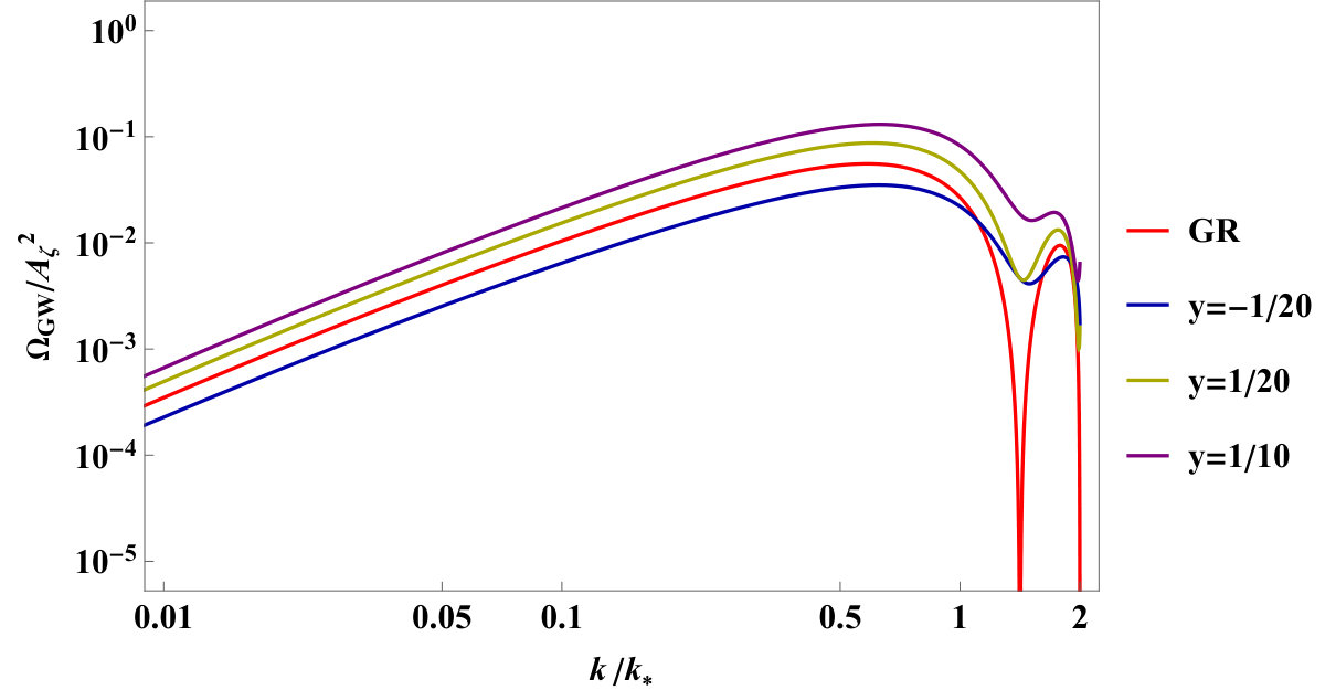 Figure 1
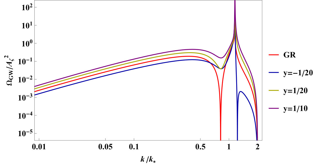 Figure 2
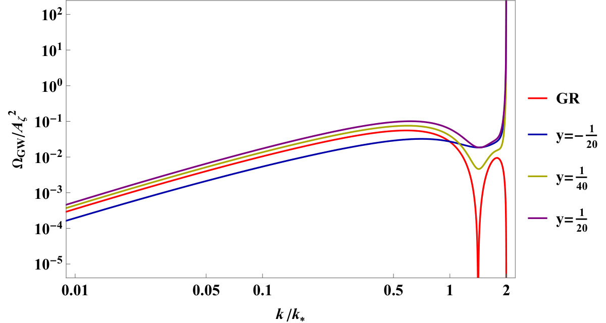 Figure 3
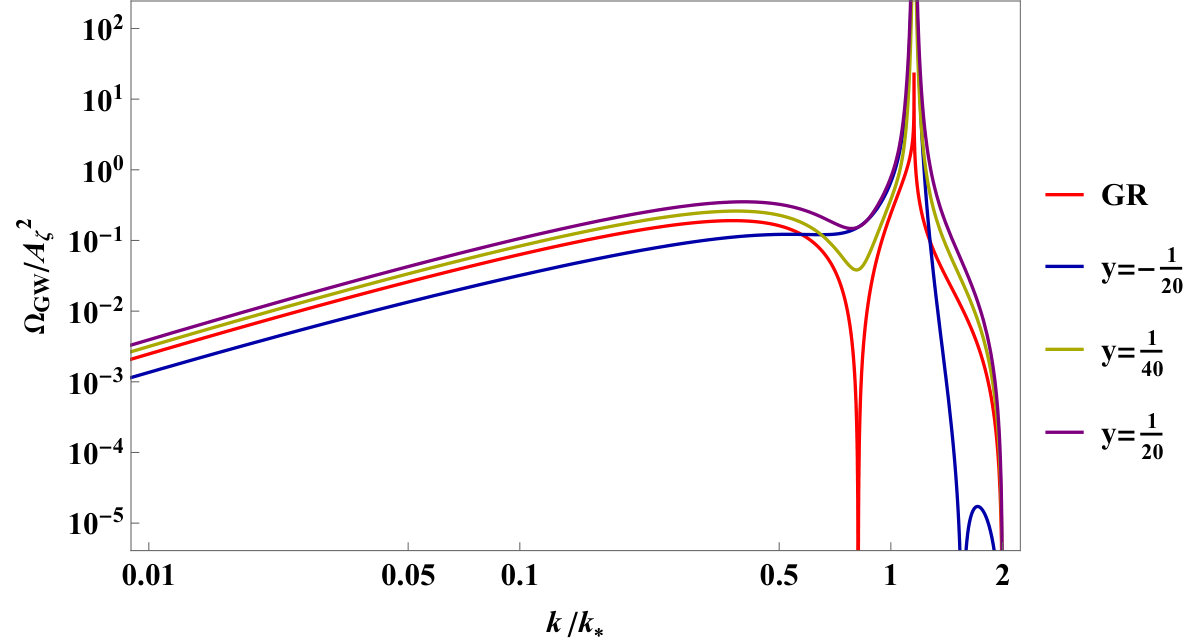 Figure 4
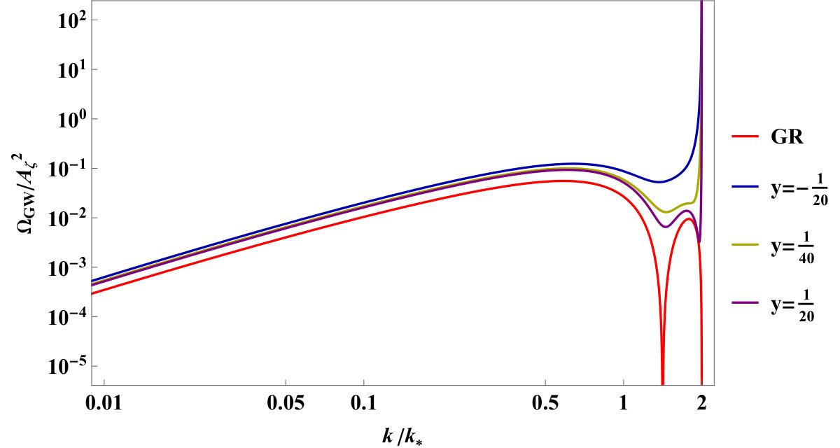 Figure 5
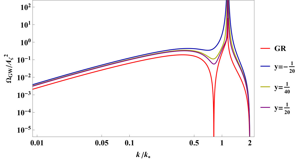 Figure 6
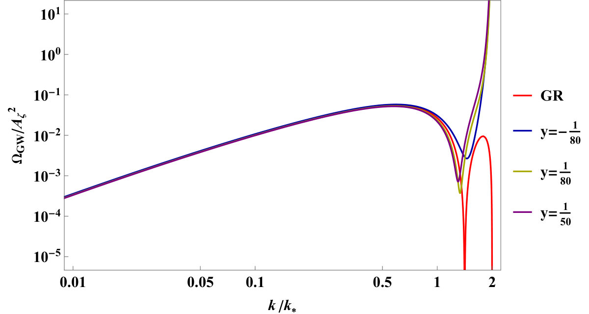 Figure 7
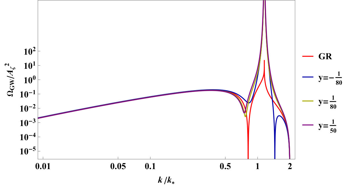 Figure 8
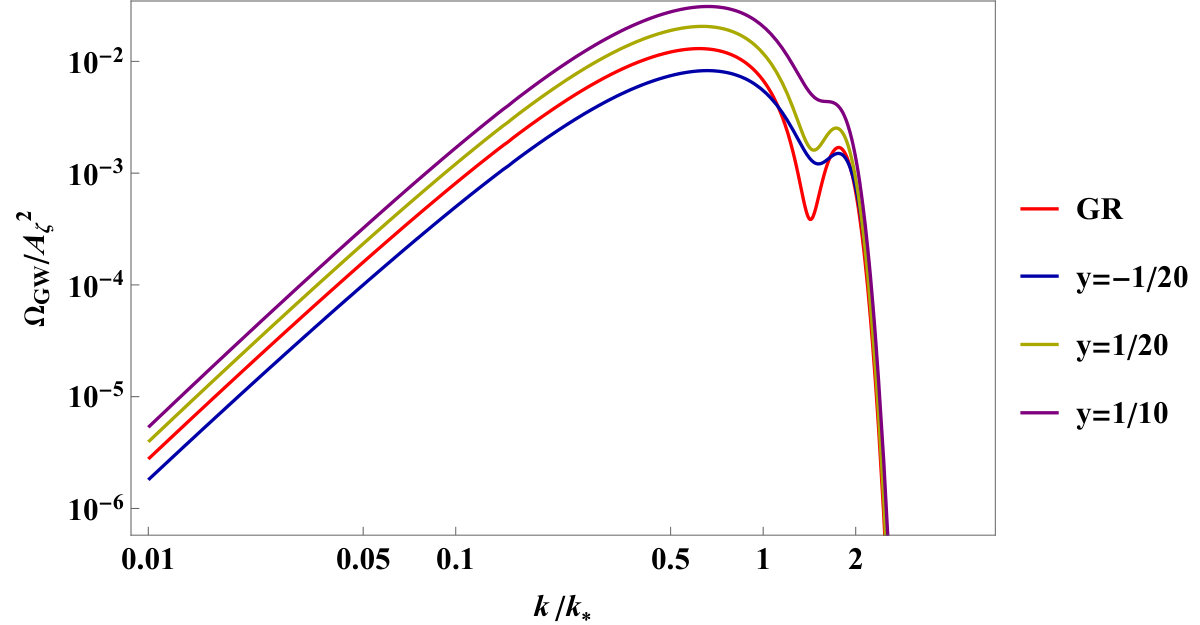 Figure 9
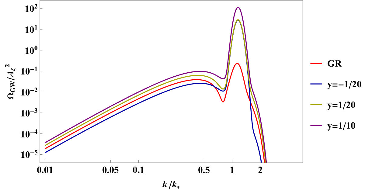 Figure 10
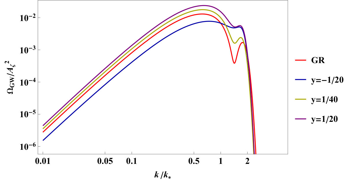 Figure 11
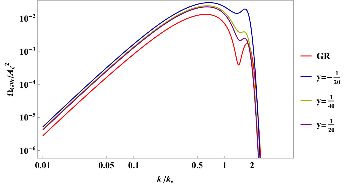 Figure 12
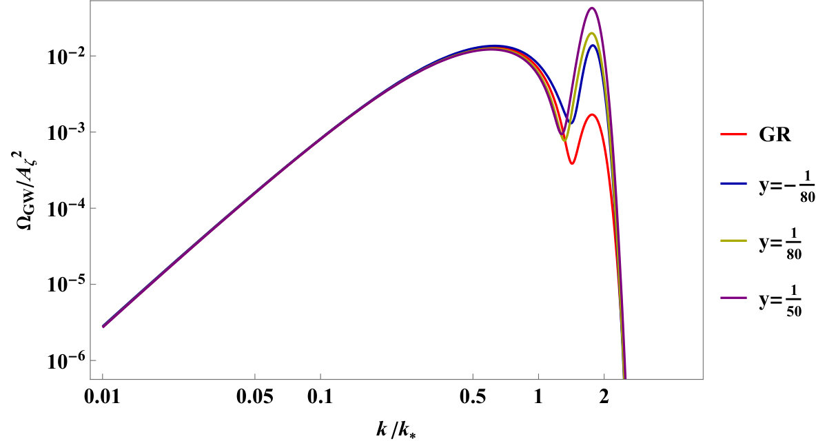 Figure 13
Peer Reviews
No public reviews on file for this paper yet. If you reviewed it on a platform where reviews are public (OpenReview, ICLR, NeurIPS, ICML), you can paste yours below so the community can read it here.
Videos
No videos yet. Explain this paper in a talk, walkthrough, or lecture? Add one.
Scalar-induced gravitational waves in spatially covariant gravity
Jiehao Jiang
School of Physics, Sun Yat-sen University, Guangzhou 510275, China
Jieming Lin
Abdus Salam Centre for Theoretical Physics, Imperial College London, Prince Consort Road, London, SW7 2AZ, UK
Xian Gao
School of Physics, Sun Yat-sen University, Guangzhou 510275, China
Abstract
We investigate scalar-induced gravitational waves (SIGWs) in the framework of spatially covariant gravity (SCG), a broad class of Lorentz-violating modified gravity theories respecting only spatial diffeomorphism invariance. Extending earlier SCG formulations, we compute the general kernel function for SIGWs on a flat Friedmann-Lemaître-Robertson-Walker background, focusing on polynomial-type SCG Lagrangians up to , where denotes the total number of derivatives in each monomial. We derive explicit expressions for the kernel in the case of power-law time evolution of the coefficients, and restrict attention to the subset of SCG operators whose tensor modes propagate at the speed of light, thereby avoiding late-time divergences in the fractional energy density of SIGWs. Instead of the usual Newtonian gauge, the breaking of time reparametrization symmetry in SCG necessitates a unitary gauge analysis. We compute the energy density of SIGWs for representative parameter combinations, finding distinctive deviations from general relativity (GR), including scale-dependent modifications to both the amplitude and the spectral shape. Our results highlight the potential of stochastic GW background measurements to probe spatially covariant gravity and other Lorentz-violating extensions of GR.
I Introduction
Einstein’s general relativity (GR) remains the standard framework for describing gravitational phenomena from the solar system to cosmological scales, having passed numerous observational tests. Nevertheless, persistent open problems motivate exploration beyond GR. From an observational perspective, the accelerated expansion of the universe [1, 2] suggests the existence of dark energy. Tension between early and late-time measurements of the Hubble constant [3, 4] also suggests the need for new physics. Modified gravity theories offer a compelling route to address these puzzles (see e.g. [5] for a review).
The detection of gravitational waves (GWs) by LIGO and Virgo [6, 7, 8, 9, 10, 11, 12, 13, 14, 15, 16] has provided a novel tool for testing gravity on cosmological scales. GWs are conventionally studied at first order as linear tensor modes generated during inflation. However, even in the absence of a large primordial tensor signal, nonlinear mode couplings ensure that scalar fluctuations inevitably generate second- or higher-order GWs, known as scalar-induced gravitational waves (SIGWs) [17, 18, 19, 20]. Recent observations from pulsar timing arrays (PTAs), including NANOGrav [21, 22, 23, 24, 25, 26], PPTA [27], EPTA [28], and CPTA [29], have reported a common-spectrum stochastic signal in the nanohertz band that can be interpreted in terms of SIGWs [30, 31, 32, 33, 34, 35, 36, 37]. Forthcoming space-based interferometers such as LISA [38], DECIGO [39], Taiji [40] and TianQin [41] will further expand sensitivity to SIGWs across a wide frequency range.
Because SIGWs are generated during horizon re-entry of enhanced scalar perturbations, they can serve as a powerful probe of both the small-scale primordial power spectrum and modifications to the underlying gravitational theory [42, 43, 44, 45, 46, 47, 48, 49, 50, 51, 52, 53, 54, 55, 56, 57, 58, 59, 60, 61, 62, 63, 64, 65, 66, 67, 68, 69, 70, 71, 72, 73, 74, 75]. Moreover, connections to primordial black hole (PBH) formation [76, 77, 78, 79, 80, 81, 82, 83, 84, 85, 86, 87, 88] have also heightened the importance of SIGWs. SIGWs depend on nonlinear mode coupling and thus can probe interaction terms that leave linear dynamics unchanged. In modified gravity theories, both the evolution of scalar and tensor perturbations themselves and the coupling between the scalar and tensor modes can differ from those in GR, resulting in different SIGW predictions. Analyses have been performed for Brans-Dicke theory [82], gravity [89, 90], Gauss-Bonnet models [56], Horndeski theory [91], and modified teleparallel gravity [92]. In particular, parity-violating (PV) gravity theories are of special interest, which predict possible circular polarization in the SIGW background. The SIGWs in PV gravity have been studied extensively [93, 94, 95, 96, 97, 98, 99]. See [100] for a recent review and more references therein.
In this work, we focus on SIGWs in spatially covariant gravity (SCG), a general class of modified gravity theories respecting only the spatial covariance [101, 102]. In this sense, effective field theory of inflation [103, 104] and dark energy [105] as well as the Hořava gravity [106, 107] can be viewed as special cases of SCG. One important advantage of SCG is that due to the separation between space and time derivatives, it is feasible to build theories with the desired degrees of freedom (DOFs). In its simplest form without higher time derivatives, SCG propagates 3 DOFs (two tensor and one scalar), and thus has a natural correspondence to the single-field scalar-tensor theories [108, 109, 110, 111, 112].
Cosmological perturbations and linear GWs in SCG theories have been extensively studied [113, 114, 115, 116]. See also [117, 118, 119, 120, 121, 122, 123, 124] for constraints on Lorentz violation from GWs. Since SCG generically breaks Lorentz invariance, it allows a richer set of operators than covariant theories, many of which remain viable after GW170817 constraints [114]. In particular, SCG modifies both the scalar and tensor perturbation sectors, altering the cubic interactions that source SIGWs. Unlike in GR, the kernel function in SCG can depend explicitly on the lapse and extrinsic curvature operators, introducing new time-dependent couplings.
In this work, we focus on a class of polynomial-type SCG Lagrangians up to , where is the total number of derivatives in each monomial. We follow the standard second-order cosmological perturbation theory to derive the general form of the equations of motion for SIGWs in SCG. Since there is no time reparametrization symmetry in SCG, we are not allowed to work in the Newtonian gauge that is commonly employed in the investigation of SIGWs. Instead, since SCG can be equivalently viewed as the gauge-fixed version of a scalar-tensor theory, we work in the so-called unitary gauge.
Using Green’s function methods, we derive the general kernel function governing SIGW production, with explicit dependence on SCG operators. Assuming power-law time dependence of the coefficients in the Lagrangian, we can obtain explicit solutions for the kernel function. We then concentrate on the contributions from SCG to the SIGWs during the radiation-dominated era. To be specific, we will compute the energy density of SIGWs for SCG operators with luminal tensor modes, and explore parameter combinations illustrating deviations from GR. As we will see, the SCG produces distinctive deviations from GR in the fractional energy density of SIGWs.
This paper is organized as follows. In Sec. II, we briefly review the SCG framework and specify the model we consider. In Sec. III, we introduce the cosmological perturbations and derive the equations of motion for the background evolution as well as the linear scalar and tensor perturbations. In Sec. IV, we compute the cubic action involving one tensor and two scalar perturbations, and derive the equations of motion for the SIGWs and in particular the source term and the kernel function. In Sec. V, we evaluate the energy density of SIGWs for representative parameter choices, considering both monochromatic and log-normal primordial scalar spectra, and highlight key deviations from GR. We summarize and discuss implications in Sec. VI.
II Spatially covariant gravity
Spatially covariant gravity (SCG) is defined as a class of gravity theories respecting only the spatial covariance. The general action of SCG takes the form111By definition, the SCG action (1) describes a single foliation of spacetime. It is possible to generalize it to the case with multiple foliations, which corresponds to the case with multiple scalar fields [125]. Moreover, here we consider only the Riemannian geometry, in which the metric variables are the only variables to build the theory. The SCG can be generalized to the case with an independent connection [126].
[TABLE]
Here and are the lapse function and 3-dimensional spatial metric in the usual 3+1 or Arnowitt-Deser-Misner (ADM) formalism. They are related to the 4-dimensional spacetime metric through
[TABLE]
or in terms of components
[TABLE]
where is the shift vector. In (1), is the extrinsic curvature defined by
[TABLE]
where is the Lie derivative with respect to the normal vector (as a 4-dimensional vector) to the spacelike hypersurfaces. The 3-dimensional Ricci tensor and 3-dimensional covariant derivative are naturally included in SCG. In addition, the spatial Levi-Civita tensor (with ) is also allowed in general, which will introduce parity-violating effects.
The action (1) is too general to make definitive calculations for the cosmological perturbations and in particular the scalar-induced gravitational waves. In the rest of this paper, we concentrate on a more concrete model of SCG, of which the Lagrangian is a polynomial built of , and their spatial derivatives (i.e., without higher temporal derivatives). To be precise, the action is given by [102, 113]
[TABLE]
with
[TABLE]
where
[TABLE]
[TABLE]
[TABLE]
[TABLE]
and
[TABLE]
Throughout this paper, and stand for 3-dimensional Ricci tensor and scalar, respectively. We classify monomials by numbers of derivatives, in which in counts the total number of derivatives in each monomial. See [127] for a detailed classification for more general SCG monomials. In the above, coefficients can be general functions of and . Note that has included the same monomials that appear in the 3+1 decomposition of GR but with general coefficients (as functions of ).
Here we exclude the spatial Levi-Civita tensor which leads to parity violation. The SCG with parity violation and in particular the polarized linear GWs are investigated in [114]. See also [128] for a recent discussion on more general SCG monomials with parity violation and their correspondence to the scalar-tensor theory. We also exclude the spatial derivative of the lapse function, i.e., the acceleration .
Although we have focused on the concrete model (5) with a polynomial-type Lagrangian, it is still too general and involved to calculate the cosmological perturbations. To get a better understanding of features of SIGW in SCG, in the following we make a couple of assumptions on the general action (5).
First, we assume while all other coefficients are functions of only for simplicity. Second, due to the large number of monomials in , in the following we consider the Lagrangian up to , which actually has already shown characteristic features of SIGWs from SCG. Third, we assume that the SCG deviates from GR slightly, i.e., all the coefficients in and are treated as small parameters while for coefficients in , we assume are small with . We emphasize that this “small-deviation” assumption is both physically and technically motivated. Physically, modified gravity theories are already constrained by cosmological and gravitational-wave observations, so it is natural to explore the vicinity of GR as a conservative baseline. Technically, treating , and as small ensures that the background and linear dynamics remain close to GR, so that the radiation-era transfer function can be used at leading order, while allowing characteristic SCG interactions to appear already in the kernel through the cubic terms. In addition to this “small-deviation” assumption, our parameter space is constrained by the existence of a radiation-dominated background, and the requirement of a healthy tensor sector together with observational consistency of GW propagation speed.
In order to get the solution of SIGWs with general equation of state parameter and the speed of sound of the scalar perturbation , we introduce a -essence-like term as the matter field to make sure the existence of a radiation-dominated period. In a generally covariant language, the action of -essence is given by
[TABLE]
with . In the SCG language (i.e., when written in the so-called unitary gauge with ), we have . Therefore, we assume that takes the form
[TABLE]
where and are understood as being replaced by and , respectively. This explains the necessity of assuming to be a general function of both and . Note that if we consider only the canonical kinetic term for the scalar field, we can get an arbitrary equation of state parameter while the speed of sound is fixed to 1, because a scalar field with canonical kinetic term always leads to in the unitary gauge.
With the above discussion on the coefficients, the comparison with GR is rather straightforward. While the Horndeski theory can also be written in the form of (6), but with the 10 coefficients ’s fully determined by 4 independent coefficients defined in the Horndeski theory [129, 113].
III Background evolution and linear perturbations
III.1 The cosmological perturbations
When considering perturbations around a Friedmann-Lemaître-Robertson-Walker (FLRW) background, we parametrize the ADM variables as
[TABLE]
In the above, is the background value of the lapse function, is the scale factor. are scalar perturbations, and is the tensor perturbation. The Friedmann-Lemaître-Robertson-Walker background thus corresponds to
[TABLE]
Even though one can always set the background value in a general covariant theory, we cannot do it here since the SCG theory has no time-reparametrization symmetry [113, 127]. For our purposes, we suppress the vector perturbations as they are non-dynamical and decay as .
The matrix exponential is defined as
[TABLE]
where and in the following, the spatial indices in the perturbation theory are raised and lowered by and , e.g., . As usual, is defined as a traceless and transverse symmetric tensor,
[TABLE]
which just corresponds to the tensor perturbation. For simplicity, we also adopt the notation:
[TABLE]
The inverse spatial metric is given by
[TABLE]
It is straightforward to check that
[TABLE]
By using (14), we expand as
[TABLE]
where and throughout this paper, we follow the notation of [113] by denoting
[TABLE]
At this point, recall that among all the coefficients only depends on .
In terms of and after fixing the unitary gauge , we get the explicit expressions
[TABLE]
Here and .
III.2 Background evolution
In the following, we work with the conformal time defined by and use a prime to denote the derivative with respect to the conformal time, e.g., 222There may be some confusion regarding the notations. Keep in mind that primes acting on coefficients denote derivatives with respect to , as defined in (24) and (25).. The conformal Hubble parameter is defined as usual .
By expanding the action (5) around the FLRW background with respect to the perturbation variables , , and , we can get the action for the perturbations. The first-order action for the perturbations takes the form
[TABLE]
where [113]
[TABLE]
and
[TABLE]
with
[TABLE]
Requiring the vanishing of the first-order action of perturbations (29) leads to the background equations of motion, which can be written as
[TABLE]
In the above, the effective energy density and pressure are defined to be
[TABLE]
and
[TABLE]
where and are the energy density and pressure of -essence.
In this work, we are interested in the case , which corresponds to the radiation-dominated era. For simplicity, we also assume , which imposes a constraint on the coefficient . According to (35) and (37) , this yields a constraint on the coefficients
[TABLE]
During the radiation-dominated era, equation (38) leads to and . The first Friedmann equation (33) provides a strong constraint on the coefficients of SCG polynomials, which are supposed to be arbitrary functions of conformal time, by requiring that should decay as . Moreover, when evaluating the source terms of the induced gravitational waves, we will find that the combinations of coefficients ’s are rather complicated. This is because there are terms with time derivatives on tensor modes, which should be removed by integration by parts with respect to conformal time.
For simplicity, in the rest of this paper we follow a similar approach to [91] by choosing a power-law ansatz of coefficients, i.e.,
[TABLE]
In (39), are constants and decays as as expected. In addition, this ansatz is compatible with GR since ’s are constant in (conformal) time. Precisely, GR corresponds to
[TABLE]
with all other vanishing.
III.3 Linear perturbations
In the following, we derive the linear equations of motion for the scalar and tensor perturbations. Since the scalar and tensor perturbations are decoupled at linear order, we will discuss them separately.
III.3.1 Tensor perturbations
The quadratic action for the tensor perturbations takes the form
[TABLE]
where [113]
[TABLE]
After making the mode decomposition (see Appendix A), we can write the quadratic action for the polarization modes as
[TABLE]
where with are the two polarization modes for the tensor perturbations.
Variation of (41) with respect to leads to the equations of motion for the linear gravitational waves
[TABLE]
with
[TABLE]
In (46), are the constants defined in (39).
Since the current astrophysical observations have put stringent constraints on the propagating speed of the gravitational waves [10, 130], we treat (46) as a constraint on the coefficients in the Lagrangian. In the following we choose rather than a free parameter and thus the Green’s function for the tensor perturbations is the same as that of GR.
III.3.2 Scalar perturbation
The quadratic action for the scalar perturbations , and is [113]
[TABLE]
where variously defined coefficients , etc. can be found in Appendix B.
In (47), and acquire no kinetic term and thus play the role of auxiliary variables. Variation of (47) with respect to and yields the constraint equations
[TABLE]
from which we can solve and in terms of as
[TABLE]
By plugging the solutions (50) and (51) for and in , we get the effective quadratic action for the single variable , which is given by
[TABLE]
Varying (52) with respect to leads to the equations of motion for ,
[TABLE]
The evaluation of coefficients in (52) and (53) is quite involved. Fortunately, thanks to the power-law ansatz of the coefficients (39), the equation of motion for (53) reduces to be
[TABLE]
Here we have deliberately separated terms involving into two parts.
Since we assume that the deviation of our model from GR is small, it is a good approximation to use the solution for of GR when evaluating the SIGWs. If we solve (54) perturbatively and write with the correction to the solution in GR, the contribution from to the SIGWs will be of subleading order, since SIGWs are sourced by terms of order . Hence, we can drop the contribution of .
In the case of GR (see (40)), the last term in (54) is identically vanishing. Therefore, (54) reduces to
[TABLE]
where
[TABLE]
is the well-known speed of sound of the scalar perturbation in -essence. In this case, the solution of (55) is given by
[TABLE]
where is the spherical Bessel function.
IV Cubic action and equations of motion for SIGWs
IV.1 Cubic action
In this section, we derive the equation of motion for the tensor perturbations induced from the scalar perturbations. There are two equivalent approaches. The traditional approach is to first derive the equations of motion for the ADM variables and then expand to the second order in scalar perturbations. The more convenient approach is to expand the original action up to the cubic order and focus on the part involving one tensor and two scalar modes. Then by varying the relevant cubic action, one may get the equations of motion for the tensor modes sourced by the quadratic scalar modes.
After some manipulations, the cubic action for one tensor and two scalar perturbations in momentum space is given by
[TABLE]
where the coefficients , etc. can be found in Appendix C, , and are momenta of the relevant modes. Note in (58), due to the conservation of momenta.
We can now replace the auxiliary variables and in terms of in the cubic action (58). Note that up to the cubic order in perturbations, the first order solutions (50) and (51) are sufficient. For later convenience, we follow the convention of [19, 20] and define two dimensionless parameters and . A technical issue arises when simply replacing and by their first order solutions, which generally leads to a source function that will change under the exchange if we use integration by parts inappropriately to simplify the cubic action. To get a standard source function , we need to symmetrize terms in and to be
[TABLE]
where and stand for the scalar perturbations (i.e., , or ).
After polarization decomposition, the cubic action in the radiation-dominated era can be written as
[TABLE]
where we have used for the radiation-dominated era. The explicit expressions of the coefficients etc. can be found in Appendix C.
By combining the quadratic action for the tensor modes (44), the cubic action leads to the equations of motion for the SIGWs
[TABLE]
where is the source term quadratic in the scalar perturbation . Following the steps of [70] and considering the solution of in (57), the source term can be written as
[TABLE]
The source function depends on the concrete model, which is quite complicated in our case.
Equation (61) can be simplified by introducing :
[TABLE]
which can be solved by the Green’s function method
[TABLE]
or equivalently
[TABLE]
We follow the convention of [62] to calculate the power spectrum for the tensor modes, which is defined by
[TABLE]
and the concrete expression of can be obtained by using the solution (65) for , though the calculation is quite involved. After some simplification, we arrive at [62]
[TABLE]
where
[TABLE]
is the kernel function in which the information of the Green’s function and the source is encoded, and is the power spectrum of scalar perturbation defined by
[TABLE]
In the following, we focus on the case of in order to obtain an explicit expression for the source function and a better understanding of the kernel. Later we will numerically evaluate the case of and show the power spectrum in figures.
By using the power-law solutions and , with the transfer function of the scalar perturbation given in (57), the source function can be written as
[TABLE]
where
[TABLE]
Here are functions of momenta and their explicit expressions are given in Appendix D. In (70), terms like will contribute to higher orders of . Unfortunately, we cannot find a simple solution where these terms vanish because they are functions of momenta , and in general.
Thus the source function can be written in the following form (with )
[TABLE]
where the expressions for are given in Appendix D. The source function shares the same general form as that of [91]. The coefficients satisfy as expected but contain extra terms that will contribute to higher orders of . This will lead to an apparent late-time divergence as we will discuss later.
IV.2 More on the source function and the kernel
In the following, we analyze the source function and kernel in more detail. We first isolate the GR contribution in the unitary gauge as a reference, and then extend the discussion to the full SCG case with general polynomial operators.
IV.2.1 GR part
The cubic action (60) contains a number of coefficients, which is complicated to be analyzed. Usually, the SIGWs are evaluated in the Newtonian gauge. The SCG corresponds to a generally covariant scalar-tensor theory written in the unitary gauge. In order to get some important features in the unitary gauge, we first consider the GR part of the cubic action,
[TABLE]
where we have used integration by parts with respect to the conformal time to eliminate time derivatives on tensor modes. The coefficients ’s are functions of conformal time and momenta and , which are different from those in the Newtonian gauge where all the coefficients are simply functions of conformal time. Note that the last two terms in the third line of (77) contain three temporal derivatives in total. Such terms do not appear in Newtonian gauge.
The GR part of the source function in the unitary gauge can be written as
[TABLE]
Note the expression of is manifestly symmetric in .
The GR part of the kernel is
[TABLE]
Note that there are terms in the fourth line of (79), which diverges when taking a late-time limit . This apparent divergence does not signal a growth of the GW signal. In a generally covariant theory such as GR, the late-time observable is gauge invariant, and the apparently divergent terms that arise in the unitary gauge cancel in gauge-invariant quantities [91]. Equivalently, one may perform the second-order gauge transformation to Newtonian gauge, in which the late-time kernel contains only the standard luminal (finite) contributions. However, SCG respects only the spatial covariance and time reparametrization invariance is absent, so we cannot switch to the Newtonian gauge within the same theory. The unitary gauge is instead the natural description of the SCG action. Nevertheless, the identification of the physical SIGW signal remains robust. The observable stochastic background is carried by the freely propagating tensor modes with propagation speed , while the additional pieces correspond to non-luminal or “strain” contributions associated with scalar-tensor mixing. This motivates the separation of the kernel into luminal (finite) and non-luminal (potentially divergent) parts in the general SCG case discussed next.
IV.2.2 SCG with general polynomials
After integrating the Green’s function with the power-law ansatz, the kernel of SCG theory with general polynomials takes the form
[TABLE]
where
[TABLE]
and
[TABLE]
In the above, we separate the kernel into two parts. stands for “ordinary” terms that lead to a finite power spectrum, which we regard as the main part of the kernel. On the other hand, stands for “particular” terms that are higher order in , which may cause late-time divergence and include terms oscillating as .
The appearance of the structure in can be viewed as a violation of Huygens’ principle. For the luminal propagation of a massless field, the retarded Green’s function has support on the light cone, whereas non-luminal propagation generically allows “tail” support inside the light cone. The phase reflects precisely such non-luminal contributions in the effective description. It is these terms that can produce apparent late-time growth of . In this work we are interested in the stochastic background carried by the freely propagating tensor modes. Accordingly, we will extract the luminal component and discard the non-luminal strain contributions. We emphasize that we cannot directly attribute the presence of these non-luminal contributions (and thus the intra-cone GW modes that violate the Huygens’ principle) to thee breaking Lorentz symmetry. In fact, such non-luminal oscillatory terms also appear in GR, though in the Newtonian gauge they are not present at the leading order [91, 131, 132].
The analytical expressions of are very lengthy and tedious, and we prefer not to present them in the paper. Note that in the Newtonian gauge, all the terms oscillating in are excluded at late times because they do not appear at the leading order of . This provides an explicit diagnostic for what we mean by the luminal SIGW component. At late times, it is the part scaling as (or decaying faster) and oscillating with the GW phase (more generally ), which is precisely the component computed directly in Newtonian gauge in covariant theories. The additional terms collected in are therefore identified as non-luminal contributions in unitary gauge, which are the origin of the apparent late-time divergences.
V Energy density of SIGWs
As mentioned above, (80) generically contains pieces that can yield apparent late-time divergences in . These divergences originate from the particular component , whose oscillatory structure corresponds to non-luminal contributions from the strain components induced by scalar-tensor mixing. Following the physical criterion advocated in the literature, we identify the SIGW signal with the freely propagating tensor modes, i.e. the luminal component that propagates with the GW speed (here we have chosen ) [133]. This means that we keep the late-time luminal part of the kernel (the contribution scaling as or faster) and discard the pieces responsible for the divergence. Equivalently, for the phase, only the condition contributes to the luminal propagation. All other contributions are excluded from . With this luminal projection, the remaining kernel decays as , and the fractional energy density approaches a finite late-time limit.
We follow the formalism of [62] and write the power spectrum of tensor perturbations as
[TABLE]
where and Since is absent in the kernel, we will use the parameters
[TABLE]
and in the following sections, which we all assume to be small parameters. We thus take and as a controlled expansion around GR. The admissible coefficient space is not arbitrary. The radiation-era background requires the constraint (38), and we additionally impose the luminal tensor condition (46).
In the following, we vary one particular subset of coefficients at a time, and set others to their GR values or to zero. This will diagnose which SCG terms dominantly reshape the fractional energy density of SIGWs. We will discuss two cases of the primordial spectrum for the scalar perturbation, one is the monochromatic spectrum, the other is the log-normal spectrum.
V.1 Monochromatic primordial spectrum
We first consider a monochromatic primordial spectrum for the curvature perturbation in the form of a Dirac delta function
[TABLE]
which represents an extremely narrow enhancement of scalar power centered at .
In the case of GR, when , the corresponding analytic expression for the energy density of SIGWs in the unitary gauge is given by [62]
[TABLE]
The Heaviside factor arises from momentum conservation as in the Newtonian gauge. In other words, it enforces the triangle condition , manifesting as a sharp cut-off in space.
In the case of SCG, the explicit expression for the fractional energy density is rather lengthy. In the following we simply show the numerical results with different choices of values of the coefficients. We have a total of 8 parameters (i.e., coefficients in the Lagrangian) in and , but not all choices of these parameter values are accessible. In what follows, we focus on several interesting choices of parameters and show the energy density of SIGWs.
V.1.1 Case 1:
First we consider the case with , where is constant. This case corresponds to a generally covariant limit of SCG.
As shown in figure 1, for , positive produces a nearly uniform enhancement of the SIGW amplitude across the allowed range, while negative yields a global suppression. The spectral shape remains similar to that in GR, preserving the sharp drop beyond due to momentum conservation.
For , the modification is more scale-dependent: positive not only raises the overall amplitude but also amplifies the feature near , producing a pronounced peak-like growth before the cutoff. This peak can be traced to the strong response of the SCG kernel when both scalar modes re-enter the horizon at nearly equal times, thereby enhancing the convolution integral in (83). The appearance of such sharp-edge amplification is absent in GR, indicating a genuine SCG-specific cubic-interaction effect.
V.1.2 Case 2: ,
In SCG, coefficients in can generally deviate from the values in the 3+1 decomposition of GR. We now consider the case of , and for simplicity we also assume . Here and in what follows, coefficients in that are not specified take the same value as those in GR. For example, here we choose .
In figure 2, with , a positive enhances the entire power spectrum and the shape of the spectrum is not significantly influenced. The “valley” feature in GR around is smoothed out, indicating modified interference between scalar source terms at different momenta. For negative , the suppression is strongest near , shifting the location of the minimum slightly, a sign that the SCG Lagrangian affects the effective phase velocities in the kernel.
For , the effect is more dramatic. When , the spectrum tends toward a divergence. This can be traced to contributions from terms in oscillating with at nearly zero phase velocity difference, which in SCG are not exactly canceled as in GR due to reduced symmetry. Physically, this signals that, in the unitary gauge formulation of SCG, certain cubic couplings allow “slow” tensor modes to resonate with scalar modes, enhancing the edge behavior.
V.1.3 Case 3: , ,
We now consider the case of , , where and are two constants with . Figure 3 illustrates the interplay between and .
When , spectra retain the GR-like overall shape but shift in amplitude depending on the sign of . The interference pattern (peaks and troughs) is slightly phase-shifted, which can be attributed to the mismatch between the quadratic and cubic SCG coefficients.
For , a positive again leads to edge growth near , but less violently than in Case 2, suggesting partial cancellation between - and -dependent terms in the kernel.
V.1.4 Case 4: ,
The last case we consider is the combination of coefficients as those in the Horndeski theory. Unfortunately, we have not found another choice of coefficients that leads to a power spectrum that vanishes at large scales (), and most choices blow up at large scales.
In figure 4, the Horndeski-inspired parameter choice produces a qualitatively different outcome. For , the spectrum remains finite but exhibits a steep rise as , unlike the flat IR plateau in GR. This IR growth arises because the SCG cubic vertices in this combination leave a residual constant term in that integrates to a nonzero limit as .
For , this case still avoids the sharp divergence at , but yields an intermediate- enhancement, reflecting the Horndeski structure’s tendency to suppress high interference while boosting moderate momentum transfer.
Across all cases, SCG parameters control both the global amplitude and the detailed interference patterns of the SIGW spectrum. The sharp-edge enhancement near for is a robust SCG signature whenever cubic terms fail to cancel “slow” oscillatory kernel pieces — something absent in GR due to full diffeomorphism invariance. For , changes are smoother, dominated by amplitude rescaling and valley suppression/shift. These features, if observed in future high-frequency GW measurements, could serve as direct probes of SCG operator structure.
V.2 Log-normal primordial spectrum
We now consider a log-normal primordial curvature spectrum
[TABLE]
where represents a finite-width peak. This smooth profile removes the sharp cutoff at , so interference patterns from the kernel are blended over a broader range of , and any resonant enhancement is less singular.
Unfortunately, there are no analytical expressions for in this case. Thus we will perform the integration numerically and give the results of 4 concrete cases of coefficients. Without loss of generality, in the following we set .
V.2.1 Case 1:
Figure 5 shows that for , positive produces a nearly scale-independent enhancement over the GR curve, while negative yields a mild suppression.
For , the finite width of smears the edge peak into a broader shoulder, reducing the visual sharpness but still yielding a noticeable high- excess for positive .
V.2.2 Case 2: ,
In contrast to Case 1, we find that the spectrum diverges when . Therefore in the following cases we focus on the case of .
In figure 6, positive lifts the spectrum primarily in the central -range , leaving the tails closer to the GR baseline. This suggests that the SCG modifications here act most strongly when both scalar source modes have wavenumbers near the peak of , consistent with kernel terms in that weight near-equal most heavily.
V.2.3 Case 3: , ,
As shown in figure 7, adjusting shifts the amplitude up or down, while modulates the slope on the high- side. This asymmetry relative to the peak position reflects the interplay between quadratic and cubic modifications in redistributing power between configurations with and those with larger momentum asymmetry.
V.2.4 Case 4: ,
In figure 8, this combination yields a spectrum that is more symmetric about than the previous cases, with moderate enhancement at both low and high relative to the peak. The Horndeski-like structure appears to “flatten” the spectrum, suppressing the pronounced shoulders or valleys seen in other parameter choices.
Compared with the monochromatic spectrum case, the log-normal input smooths sharp features and reduces sensitivity to the exact cutoff at . SCG effects manifest mainly as amplitude shifts and mild shape distortions, but high- shoulders can still appear when cubic couplings preferentially amplify near-equal- configurations. Taking into account the observations, the log-normal case suggests that distinguishing SCG from GR would require precise measurement of the shape of the SIGW bump, not just its amplitude.
VI Conclusion
We have carried out a systematic computation of scalar-induced gravitational waves in spatially covariant gravity, focusing on polynomial-type Lagrangians up to with the total number of derivatives in each monomial.
In Sec. III, we studied the background evolution and linear perturbations of the scalar and tensor modes in a cosmological background. Due to the breaking of time reparametrization symmetry of SCG, we are only allowed to work in unitary gauge instead of the Newtonian gauge usually adopted in calculating SIGWs in GR. This choice not only affects the formal structure of the perturbation equations but also introduces new couplings that play a crucial role in shaping the properties of SIGWs.
In Sec. IV, we derived the cubic action involving one tensor and two scalar modes and obtained the general equations of motion for SIGWs. From this, we extracted the source term and kernel function, whose time dependence encodes the deviations of SCG from GR. By considering power-law time evolution of the coefficients, we presented explicit results and restricted attention to operators yielding luminal tensor propagation. This restriction ensured consistency with observational bounds and avoided the spurious late-time divergences that can otherwise appear in . Compared with GR, the SCG kernels contain additional oscillatory structures and modified amplitude scaling, providing characteristic imprints in the resulting spectra.
In Sec. V, we evaluated the fractional energy density of SIGWs in two representative cases of the primordial curvature perturbation spectrum. One is the monochromatic spectrum, the other is the log-normal spectrum. We show the energy density for a couple of choices of coefficients. Our results show that SCG can produce significant departures from GR predictions, including scale-dependent amplitude shifts, enhanced edge behavior near , and modified spectral shapes. These features originate from SCG cubic interactions and the modified kernel function, which affect both the generation and propagation of SIGWs and remain even when deviations from GR are small.
The results presented in this work highlight the potential of stochastic GW background measurements to serve as sensitive probes of Lorentz-violating modifications to gravity. Future observations, ranging from pulsar timing arrays to space-based interferometers, may thus be capable of detecting or constraining these deviations. Extending the present work to include parity-violating operators, higher-order derivative terms, or couplings to additional fields would further broaden the phenomenology and provide valuable directions for testing gravity with GWs.
Acknowledgements.
We would like to thank Jia-Xi Feng and Fengge Zhang for valuable discussions. X.G. is supported by the National Natural Science Foundation of China (NSFC) under Grants No. 12475068 and No. 11975020 and the Guangdong Basic and Applied Basic Research Foundation under Grant No. 2025A1515012977.
Appendix A Decomposition of the tensor perturbation
The tensor perturbations can be decomposed into the polarization modes as
[TABLE]
where denotes the two polarization modes.
The polarization tensors are defined in terms of the polarization vectors as
[TABLE]
where satisfies and . The polarization tensors satisfy
[TABLE]
and
[TABLE]
Note we have
[TABLE]
Appendix B Coefficients of quadratic actions
The explicit expressions of the coefficients in 47 are given by
[TABLE]
where
[TABLE]
Solution to are
[TABLE]
where
[TABLE]
Coefficients in (52) are
[TABLE]
[TABLE]
[TABLE]
Appendix C Coefficients of Cubic action
Coefficients in (58) are
[TABLE]
and
[TABLE]
Coefficients in (60) are
[TABLE]
[TABLE]
[TABLE]
[TABLE]
Coefficients of terms with are
[TABLE]
[TABLE]
[TABLE]
[TABLE]
where .
Appendix D Source function
The explicit expressions of ’s in (70) are
[TABLE]
[TABLE]
[TABLE]
[TABLE]
[TABLE]
[TABLE]
[TABLE]
[TABLE]
[TABLE]
[TABLE]
where we define the combinations of coefficients that are constant with the power-law solution ansatz
[TABLE]
Various coefficients in the the source function in (76) are given by
[TABLE]
and .
The reference list from the paper itself. Each links out to its DOI / PubMed record.
- 1[1] Supernova Cosmology Project collaboration, Measurements of Ω \Omega and Λ \Lambda from 42 High Redshift Supernovae , Astrophys. J. 517 (1999) 565 [ astro-ph/9812133 ]. · doi ↗
- 2[2] Supernova Search Team collaboration, Observational evidence from supernovae for an accelerating universe and a cosmological constant , Astron. J. 116 (1998) 1009 [ astro-ph/9805201 ]. · doi ↗
- 3[3] L. Verde, T. Treu and A.G. Riess, Tensions between the Early and the Late Universe , Nature Astron. 3 (2019) 891 [ 1907.10625 ]. · doi ↗
- 4[4] E. Di Valentino, O. Mena, S. Pan, L. Visinelli, W. Yang, A. Melchiorri et al., In the realm of the Hubble tension—a review of solutions , Class. Quant. Grav. 38 (2021) 153001 [ 2103.01183 ]. · doi ↗
- 5[5] A. Joyce, B. Jain, J. Khoury and M. Trodden, Beyond the Cosmological Standard Model , Phys.Rept. 568 (2015) 1 [ 1407.0059 ]. · doi ↗
- 6[6] LIGO Scientific, Virgo collaboration, GW 150914: Implications for the stochastic gravitational wave background from binary black holes , Phys. Rev. Lett. 116 (2016) 131102 [ 1602.03847 ]. · doi ↗
- 7[7] LIGO Scientific, Virgo collaboration, GW 151226: Observation of Gravitational Waves from a 22-Solar-Mass Binary Black Hole Coalescence , Phys. Rev. Lett. 116 (2016) 241103 [ 1606.04855 ]. · doi ↗
- 8[8] LIGO Scientific, Virgo collaboration, Observation of Gravitational Waves from a Binary Black Hole Merger , Phys. Rev. Lett. 116 (2016) 061102 [ 1602.03837 ]. · doi ↗