Dominant H-Eigenvectors of Tensor Kronecker Products Do Not Decouple
Ayush Kulkarni, Charles Colley, David F. Gleich

TL;DR
This paper presents a counterexample showing that the dominant H-eigenvector of a tensor Kronecker product does not always decouple into the eigenvectors of the individual tensors, contrasting with matrix and Z-eigenvector cases.
Contribution
It provides the first known counterexample for H-eigenvectors and clarifies conditions where decoupling does or does not occur.
Findings
Counterexample disproves decoupling for H-eigenvectors
Decoupling holds for diagonal and nonnegative tensors
Largest H-eigenvalue can exceed the product of component eigenvalues
Abstract
We illustrate a counterexample to an open question related to the dominant H-eigenvector of a Kronecker product of tensors. For matrices and Z-eigenvectors of tensors, the dominant eigenvector of a Kronecker product decouples into a product of eigenvectors of the tensors underlying the Kronecker product. This does not occur for H-eigenvectors and indeed, the largest H-eigenvalue can exceed the product of the H-eigenvalues of the component tensors. Beyond this general counterexample, we show this decoupling does hold in the case of diagonal tensors as well as nonnegative tensors.
Click any figure to enlarge with its caption.
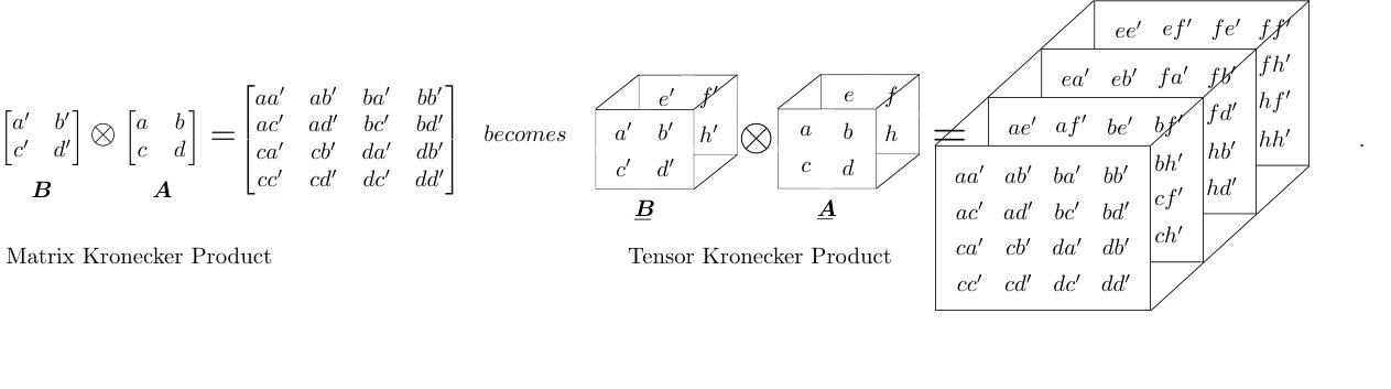 Figure 1
Peer Reviews
No public reviews on file for this paper yet. If you reviewed it on a platform where reviews are public (OpenReview, ICLR, NeurIPS, ICML), you can paste yours below so the community can read it here.
Videos
No videos yet. Explain this paper in a talk, walkthrough, or lecture? Add one.
\newsiamremark
remarkRemark \newsiamremarkhypothesisHypothesis
\newsiamthmclaimClaim \headersH-Eigenpairs and Tensor Kronecker ProductsA. Kulkarni, C. Colley, D. F.Gleich \externaldocumentex_supplement
Dominant H-Eigenpairs of Tensor Kronecker Products do not decouple††thanks: This work was funded by the DOE DE-SC0023162 Sparstitute MMICC center.
Ayush Kulkarni Metea Valley High School, Aurora, IL ().
Charles Colley Department of Computer Science, Purdue University, West Lafayette, IN (, ).
David F. Gleich33footnotemark: 3
Abstract
We illustrate a counterexample to an open question related to the dominant H-eigenvector of a Kronecker product of tensors. For matrices and Z-eigenvectors of tensors, the dominant eigenvector of a Kronecker product decouples into a product of eigenvectors of the tensors underlying the Kronecker product. This does not occur for H-eigenvectors and indeed, the largest H-eigenvalue can exceed the product of the H-eigenvalues of the component tensors. Beyond this general counterexample, we show this decoupling does hold in the case of diagonal tensors as well as nonnegative tensors.
keywords:
Kronecker product, H-eigenvector, tensor eigenvector
{AMS}
15A69, 15A18, 15A72, 65F15
1 Introduction
In Colley-2023-tensor-kron, we showed that the dominant tensor -eigenvector of a Kronecker product of tensors \mathchoice{\hbox to0.0pt{{\underline{{\hbox to6.00003pt{}}}\hss}}}{\hbox to0.0pt{{\underline{{\hbox to6.00003pt{}}}\hss}}}{\hbox to0.0pt{{\underline{{\hbox to4.72226pt{}}}\hss}}}{\hbox to0.0pt{{\underline{{\hbox to3.9223pt{}}}\hss}}}\bm{{A}} and \mathchoice{\hbox to0.0pt{{\underline{{\hbox to5.6667pt{}}}\hss}}}{\hbox to0.0pt{{\underline{{\hbox to5.6667pt{}}}\hss}}}{\hbox to0.0pt{{\underline{{\hbox to4.47224pt{}}}\hss}}}{\hbox to0.0pt{{\underline{{\hbox to3.73895pt{}}}\hss}}}\bm{{B}} can be expressed as the Kronecker product of the dominant tensor -eigenvectors of \mathchoice{\hbox to0.0pt{{\underline{{\hbox to6.00003pt{}}}\hss}}}{\hbox to0.0pt{{\underline{{\hbox to6.00003pt{}}}\hss}}}{\hbox to0.0pt{{\underline{{\hbox to4.72226pt{}}}\hss}}}{\hbox to0.0pt{{\underline{{\hbox to3.9223pt{}}}\hss}}}\bm{{A}} and \mathchoice{\hbox to0.0pt{{\underline{{\hbox to5.6667pt{}}}\hss}}}{\hbox to0.0pt{{\underline{{\hbox to5.6667pt{}}}\hss}}}{\hbox to0.0pt{{\underline{{\hbox to4.47224pt{}}}\hss}}}{\hbox to0.0pt{{\underline{{\hbox to3.73895pt{}}}\hss}}}\bm{{B}}, respectively. Our result mirrors a theorem about matrix eigenvectors and Kronecker products. Here, we show that this statement is false in general for -eigenvectors of tensors via a counterexample, which resolves a question that arose in the review of Colley-2023-tensor-kron.
The tensor Kronecker product generalizes the Kronecker product of matrices as follows
[TABLE]
We use the increasingly standard notation where
[TABLE]
Then a -eigenvector of a -mode symmetric tensor is any solution of
[TABLE]
whereas an -eigenvector (see note below on vs ) of a tensor is any solution of
[TABLE]
For more on these, see Qi-2005-Z-eigenvalues; Lim-2005-eigenvalues. One key difference is that for -eigenvectors, the spectrum is invariant to the scale of the vector, whereas this is not the case for -eigenvectors. Note that, strictly speaking, Qi-2005-Z-eigenvalues defines -eigenvalues and eigenvectors as real and uses the term eigenvalue and eigenvector to represent real and complex cases. We use the terms -eigenvalue or -eigenvector to represent real or complex solutions of (2) to clearly distinguish from the -eigenvector case.
Let be the spectral radius of a matrix, which is the largest magnitude of any eigenvalue. It is well-known that for matrices, and moreover, that the eigenvector that achieves the spectral radius is a Kronecker product of the eigenvectors of and .
This theorem generalizes to -eigenvectors of tensors as well. {theorem*}[From Colley-2023-tensor-kron] Let \mathchoice{\hbox to0.0pt{{\underline{{\hbox to6.00003pt{}}}\hss}}}{\hbox to0.0pt{{\underline{{\hbox to6.00003pt{}}}\hss}}}{\hbox to0.0pt{{\underline{{\hbox to4.72226pt{}}}\hss}}}{\hbox to0.0pt{{\underline{{\hbox to3.9223pt{}}}\hss}}}\bm{{A}} be a symmetric, -mode, -dimensional tensor and \mathchoice{\hbox to0.0pt{{\underline{{\hbox to5.6667pt{}}}\hss}}}{\hbox to0.0pt{{\underline{{\hbox to5.6667pt{}}}\hss}}}{\hbox to0.0pt{{\underline{{\hbox to4.47224pt{}}}\hss}}}{\hbox to0.0pt{{\underline{{\hbox to3.73895pt{}}}\hss}}}\bm{{B}} be a symmetric, -mode, -dimensional tensor. Suppose that and are any dominant tensor -eigenvalues and vectors of \mathchoice{\hbox to0.0pt{{\underline{{\hbox to6.00003pt{}}}\hss}}}{\hbox to0.0pt{{\underline{{\hbox to6.00003pt{}}}\hss}}}{\hbox to0.0pt{{\underline{{\hbox to4.72226pt{}}}\hss}}}{\hbox to0.0pt{{\underline{{\hbox to3.9223pt{}}}\hss}}}\bm{{A}} and \mathchoice{\hbox to0.0pt{{\underline{{\hbox to5.6667pt{}}}\hss}}}{\hbox to0.0pt{{\underline{{\hbox to5.6667pt{}}}\hss}}}{\hbox to0.0pt{{\underline{{\hbox to4.47224pt{}}}\hss}}}{\hbox to0.0pt{{\underline{{\hbox to3.73895pt{}}}\hss}}}\bm{{B}}, respectively. Then is a largest magnitude eigenpair of \mathchoice{\hbox to0.0pt{{\underline{{\hbox to5.6667pt{}}}\hss}}}{\hbox to0.0pt{{\underline{{\hbox to5.6667pt{}}}\hss}}}{\hbox to0.0pt{{\underline{{\hbox to4.47224pt{}}}\hss}}}{\hbox to0.0pt{{\underline{{\hbox to3.73895pt{}}}\hss}}}\bm{{B}}\otimes\mathchoice{\hbox to0.0pt{{\underline{{\hbox to6.00003pt{}}}\hss}}}{\hbox to0.0pt{{\underline{{\hbox to6.00003pt{}}}\hss}}}{\hbox to0.0pt{{\underline{{\hbox to4.72226pt{}}}\hss}}}{\hbox to0.0pt{{\underline{{\hbox to3.9223pt{}}}\hss}}}\bm{{A}}. Moreover, any Kronecker product of -eigenvectors of \mathchoice{\hbox to0.0pt{{\underline{{\hbox to6.00003pt{}}}\hss}}}{\hbox to0.0pt{{\underline{{\hbox to6.00003pt{}}}\hss}}}{\hbox to0.0pt{{\underline{{\hbox to4.72226pt{}}}\hss}}}{\hbox to0.0pt{{\underline{{\hbox to3.9223pt{}}}\hss}}}\bm{{A}} and \mathchoice{\hbox to0.0pt{{\underline{{\hbox to5.6667pt{}}}\hss}}}{\hbox to0.0pt{{\underline{{\hbox to5.6667pt{}}}\hss}}}{\hbox to0.0pt{{\underline{{\hbox to4.47224pt{}}}\hss}}}{\hbox to0.0pt{{\underline{{\hbox to3.73895pt{}}}\hss}}}\bm{{B}} is a -eigenvector of \mathchoice{\hbox to0.0pt{{\underline{{\hbox to5.6667pt{}}}\hss}}}{\hbox to0.0pt{{\underline{{\hbox to5.6667pt{}}}\hss}}}{\hbox to0.0pt{{\underline{{\hbox to4.47224pt{}}}\hss}}}{\hbox to0.0pt{{\underline{{\hbox to3.73895pt{}}}\hss}}}\bm{{B}}\otimes\mathchoice{\hbox to0.0pt{{\underline{{\hbox to6.00003pt{}}}\hss}}}{\hbox to0.0pt{{\underline{{\hbox to6.00003pt{}}}\hss}}}{\hbox to0.0pt{{\underline{{\hbox to4.72226pt{}}}\hss}}}{\hbox to0.0pt{{\underline{{\hbox to3.9223pt{}}}\hss}}}\bm{{A}}.
2 Counterexamples
We show one counterexample and one false counterexample. The first is a simple and most general case that is worked out in full detail. It has real-valued dominant eigenvalues and we are able to get analytic solutions for everything. The second false counterexample illustrates why we want to view -eigenvalues as taking real or complex values. This example would be a counterexample for a strict real-valued definition of -eigenvalues but would not be a counter-example for the more general complex-valued case we study.
To establish our counterexamples, we need to recall a theorem from Qi-2005-Z-eigenvalues regarding the number of -eigenvalues of a tensor. {theorem*}[Paraphrased from Qi-2005-Z-eigenvalues, Theorem 1, parts (a,b)] Let \mathchoice{\hbox to0.0pt{{\underline{{\hbox to6.00003pt{}}}\hss}}}{\hbox to0.0pt{{\underline{{\hbox to6.00003pt{}}}\hss}}}{\hbox to0.0pt{{\underline{{\hbox to4.72226pt{}}}\hss}}}{\hbox to0.0pt{{\underline{{\hbox to3.9223pt{}}}\hss}}}\bm{{A}} be a symmetric tensor with modes and dimensions in each mode. (a) A number is an eigenvalue (-eigenvalue over ) of \mathchoice{\hbox to0.0pt{{\underline{{\hbox to6.00003pt{}}}\hss}}}{\hbox to0.0pt{{\underline{{\hbox to6.00003pt{}}}\hss}}}{\hbox to0.0pt{{\underline{{\hbox to4.72226pt{}}}\hss}}}{\hbox to0.0pt{{\underline{{\hbox to3.9223pt{}}}\hss}}}\bm{{A}} if and only if it is a root of the characteristic polynomial \det(\mathchoice{\hbox to0.0pt{{\underline{{\hbox to6.00003pt{}}}\hss}}}{\hbox to0.0pt{{\underline{{\hbox to6.00003pt{}}}\hss}}}{\hbox to0.0pt{{\underline{{\hbox to4.72226pt{}}}\hss}}}{\hbox to0.0pt{{\underline{{\hbox to3.9223pt{}}}\hss}}}\bm{{A}}-\lambda\mathchoice{\hbox to0.0pt{{\underline{{\hbox to2.8889pt{}}}\hss}}}{\hbox to0.0pt{{\underline{{\hbox to2.8889pt{}}}\hss}}}{\hbox to0.0pt{{\underline{{\hbox to2.31113pt{}}}\hss}}}{\hbox to0.0pt{{\underline{{\hbox to1.9778pt{}}}\hss}}}\bm{{I}}) for the hyperdeterminant. (b) The number of eigenvalues (-eigenvalues over ) is . Their product is equal to \det(\mathchoice{\hbox to0.0pt{{\underline{{\hbox to6.00003pt{}}}\hss}}}{\hbox to0.0pt{{\underline{{\hbox to6.00003pt{}}}\hss}}}{\hbox to0.0pt{{\underline{{\hbox to4.72226pt{}}}\hss}}}{\hbox to0.0pt{{\underline{{\hbox to3.9223pt{}}}\hss}}}\bm{{A}}) (the hyperdeterminant).
2.1 The simple counterexample
The following pair of symmetric tensors is a counterexample. Let
[TABLE]
where the other entries are filled by symmetry. We used a number of techniques to compute and verify the -eigenvalues. For these tensors, we can analytically determine the -eigenvalues through the polynomial from the hyperdeterminant of (\mathchoice{\hbox to0.0pt{{\underline{{\hbox to6.00003pt{}}}\hss}}}{\hbox to0.0pt{{\underline{{\hbox to6.00003pt{}}}\hss}}}{\hbox to0.0pt{{\underline{{\hbox to4.72226pt{}}}\hss}}}{\hbox to0.0pt{{\underline{{\hbox to3.9223pt{}}}\hss}}}\bm{{A}}-\lambda\mathchoice{\hbox to0.0pt{{\underline{{\hbox to2.8889pt{}}}\hss}}}{\hbox to0.0pt{{\underline{{\hbox to2.8889pt{}}}\hss}}}{\hbox to0.0pt{{\underline{{\hbox to2.31113pt{}}}\hss}}}{\hbox to0.0pt{{\underline{{\hbox to1.9778pt{}}}\hss}}}\bm{{I}}). For \mathchoice{\hbox to0.0pt{{\underline{{\hbox to6.00003pt{}}}\hss}}}{\hbox to0.0pt{{\underline{{\hbox to6.00003pt{}}}\hss}}}{\hbox to0.0pt{{\underline{{\hbox to4.72226pt{}}}\hss}}}{\hbox to0.0pt{{\underline{{\hbox to3.9223pt{}}}\hss}}}\bm{{A}}, the polynomial is . For \mathchoice{\hbox to0.0pt{{\underline{{\hbox to5.6667pt{}}}\hss}}}{\hbox to0.0pt{{\underline{{\hbox to5.6667pt{}}}\hss}}}{\hbox to0.0pt{{\underline{{\hbox to4.47224pt{}}}\hss}}}{\hbox to0.0pt{{\underline{{\hbox to3.73895pt{}}}\hss}}}\bm{{B}} we have the polynomial .111To compute these expressions, we implemented the formula for the hyperdeterminant from Wikipedia and substituted in the entries of \mathchoice{\hbox to0.0pt{{\underline{{\hbox to6.00003pt{}}}\hss}}}{\hbox to0.0pt{{\underline{{\hbox to6.00003pt{}}}\hss}}}{\hbox to0.0pt{{\underline{{\hbox to4.72226pt{}}}\hss}}}{\hbox to0.0pt{{\underline{{\hbox to3.9223pt{}}}\hss}}}\bm{{A}}-\lambda\mathchoice{\hbox to0.0pt{{\underline{{\hbox to2.8889pt{}}}\hss}}}{\hbox to0.0pt{{\underline{{\hbox to2.8889pt{}}}\hss}}}{\hbox to0.0pt{{\underline{{\hbox to2.31113pt{}}}\hss}}}{\hbox to0.0pt{{\underline{{\hbox to1.9778pt{}}}\hss}}}\bm{{I}} in a symbolic computing package. As further evidence that these are correct and complete, we note that both satisfy the property that \det(\mathchoice{\hbox to0.0pt{{\underline{{\hbox to6.00003pt{}}}\hss}}}{\hbox to0.0pt{{\underline{{\hbox to6.00003pt{}}}\hss}}}{\hbox to0.0pt{{\underline{{\hbox to4.72226pt{}}}\hss}}}{\hbox to0.0pt{{\underline{{\hbox to3.9223pt{}}}\hss}}}\bm{{A}})=\prod\lambda(\mathchoice{\hbox to0.0pt{{\underline{{\hbox to6.00003pt{}}}\hss}}}{\hbox to0.0pt{{\underline{{\hbox to6.00003pt{}}}\hss}}}{\hbox to0.0pt{{\underline{{\hbox to4.72226pt{}}}\hss}}}{\hbox to0.0pt{{\underline{{\hbox to3.9223pt{}}}\hss}}}\bm{{A}})=-9/500 and \det(\mathchoice{\hbox to0.0pt{{\underline{{\hbox to5.6667pt{}}}\hss}}}{\hbox to0.0pt{{\underline{{\hbox to5.6667pt{}}}\hss}}}{\hbox to0.0pt{{\underline{{\hbox to4.47224pt{}}}\hss}}}{\hbox to0.0pt{{\underline{{\hbox to3.73895pt{}}}\hss}}}\bm{{B}})=\prod\lambda(\mathchoice{\hbox to0.0pt{{\underline{{\hbox to5.6667pt{}}}\hss}}}{\hbox to0.0pt{{\underline{{\hbox to5.6667pt{}}}\hss}}}{\hbox to0.0pt{{\underline{{\hbox to4.47224pt{}}}\hss}}}{\hbox to0.0pt{{\underline{{\hbox to3.73895pt{}}}\hss}}}\bm{{B}})=279/625 as shown in Qi’s theorem. Moreover, we have distinct values following the same theorem. Numerically, the roots of these polynomials are
[TABLE]
[TABLE]
The eigenvectors associated with each tensor are given by the following expression
[TABLE]
These expressions arise from scaling the eigenvector as (assuming ) and then solving the -eigenvector equation. For the tensor \mathchoice{\hbox to0.0pt{{\underline{{\hbox to6.00003pt{}}}\hss}}}{\hbox to0.0pt{{\underline{{\hbox to6.00003pt{}}}\hss}}}{\hbox to0.0pt{{\underline{{\hbox to4.72226pt{}}}\hss}}}{\hbox to0.0pt{{\underline{{\hbox to3.9223pt{}}}\hss}}}\bm{{A}}, this simplifies due to the value of [math] in the tensor and it becomes a simple linear equation to solve. For the tensor \mathchoice{\hbox to0.0pt{{\underline{{\hbox to5.6667pt{}}}\hss}}}{\hbox to0.0pt{{\underline{{\hbox to5.6667pt{}}}\hss}}}{\hbox to0.0pt{{\underline{{\hbox to4.47224pt{}}}\hss}}}{\hbox to0.0pt{{\underline{{\hbox to3.73895pt{}}}\hss}}}\bm{{B}}, this expansion gives two quadratic equations in we need to satisfy. We solve one for and substitute that value of into the other to get a linear function for .
We also found that HomotopyContinuation.jl (HomotopyContinuation.jl) will solve the system of equations for the -eigenvalues reliably. This software gives the same results.
Consequently, the largest magnitude -eigenvalue we would expect for the Kronecker product of \mathchoice{\hbox to0.0pt{{\underline{{\hbox to5.6667pt{}}}\hss}}}{\hbox to0.0pt{{\underline{{\hbox to5.6667pt{}}}\hss}}}{\hbox to0.0pt{{\underline{{\hbox to4.47224pt{}}}\hss}}}{\hbox to0.0pt{{\underline{{\hbox to3.73895pt{}}}\hss}}}\bm{{B}} and \mathchoice{\hbox to0.0pt{{\underline{{\hbox to6.00003pt{}}}\hss}}}{\hbox to0.0pt{{\underline{{\hbox to6.00003pt{}}}\hss}}}{\hbox to0.0pt{{\underline{{\hbox to4.72226pt{}}}\hss}}}{\hbox to0.0pt{{\underline{{\hbox to3.9223pt{}}}\hss}}}\bm{{A}} (if the theorem held for -eigenvectors) is .
The tensor Kronecker product \mathchoice{\hbox to0.0pt{{\underline{{\hbox to5.7778pt{}}}\hss}}}{\hbox to0.0pt{{\underline{{\hbox to5.7778pt{}}}\hss}}}{\hbox to0.0pt{{\underline{{\hbox to4.5667pt{}}}\hss}}}{\hbox to0.0pt{{\underline{{\hbox to3.83339pt{}}}\hss}}}\bm{{C}}=\mathchoice{\hbox to0.0pt{{\underline{{\hbox to5.6667pt{}}}\hss}}}{\hbox to0.0pt{{\underline{{\hbox to5.6667pt{}}}\hss}}}{\hbox to0.0pt{{\underline{{\hbox to4.47224pt{}}}\hss}}}{\hbox to0.0pt{{\underline{{\hbox to3.73895pt{}}}\hss}}}\bm{{B}}\otimes\mathchoice{\hbox to0.0pt{{\underline{{\hbox to6.00003pt{}}}\hss}}}{\hbox to0.0pt{{\underline{{\hbox to6.00003pt{}}}\hss}}}{\hbox to0.0pt{{\underline{{\hbox to4.72226pt{}}}\hss}}}{\hbox to0.0pt{{\underline{{\hbox to3.9223pt{}}}\hss}}}\bm{{A}} has entries
[TABLE]
The HomotopyContinuation.jl software gives the following -eigenvector
[TABLE]
One can easily verify this expression for an H-eigenvalue and vector pair holds computationally to machine precision. Since this value is larger (in magnitude) than , we have a counterexample. If we reshape this vector to a matrix, then the matrix is rank (singular values 0.995, 0.105), which shows that it is not the Kronecker product of two smaller vectors.
2.2 A counterexample over the real numbers that is not a counterexample over complex numbers
After some initial experiments, we eventually settled on HomotopyContinuation.jl to solve for both real and complex -eigenvalues, as well as the hyperdeterminant formulation. Our initial studies, however, used the AReigST software (cui2014all) for real -eigenvalues. This led to the following counterexample over real-valued -eigenvalues. We use tensors
[TABLE]
where the other entries are filled by symmetry.
Like before, we compute the characteristic polynomials symbolically. For \mathchoice{\hbox to0.0pt{{\underline{{\hbox to6.00003pt{}}}\hss}}}{\hbox to0.0pt{{\underline{{\hbox to6.00003pt{}}}\hss}}}{\hbox to0.0pt{{\underline{{\hbox to4.72226pt{}}}\hss}}}{\hbox to0.0pt{{\underline{{\hbox to3.9223pt{}}}\hss}}}\bm{{A}}, the polynomial is . For \mathchoice{\hbox to0.0pt{{\underline{{\hbox to5.6667pt{}}}\hss}}}{\hbox to0.0pt{{\underline{{\hbox to5.6667pt{}}}\hss}}}{\hbox to0.0pt{{\underline{{\hbox to4.47224pt{}}}\hss}}}{\hbox to0.0pt{{\underline{{\hbox to3.73895pt{}}}\hss}}}\bm{{B}} we have the polynomial . Numerically, the roots of these polynomials are:
[TABLE]
Using software that restricts search to real numbers, one would identify the spectral radii as the largest real eigenvalues: \rho_{\mathbb{R}}(\mathchoice{\hbox to0.0pt{{\underline{{\hbox to6.00003pt{}}}\hss}}}{\hbox to0.0pt{{\underline{{\hbox to6.00003pt{}}}\hss}}}{\hbox to0.0pt{{\underline{{\hbox to4.72226pt{}}}\hss}}}{\hbox to0.0pt{{\underline{{\hbox to3.9223pt{}}}\hss}}}\bm{{A}})=1.911703027597 and \rho_{\mathbb{R}}(\mathchoice{\hbox to0.0pt{{\underline{{\hbox to5.6667pt{}}}\hss}}}{\hbox to0.0pt{{\underline{{\hbox to5.6667pt{}}}\hss}}}{\hbox to0.0pt{{\underline{{\hbox to4.47224pt{}}}\hss}}}{\hbox to0.0pt{{\underline{{\hbox to3.73895pt{}}}\hss}}}\bm{{B}})=2.142282147691. If the theorem \rho(\mathchoice{\hbox to0.0pt{{\underline{{\hbox to5.6667pt{}}}\hss}}}{\hbox to0.0pt{{\underline{{\hbox to5.6667pt{}}}\hss}}}{\hbox to0.0pt{{\underline{{\hbox to4.47224pt{}}}\hss}}}{\hbox to0.0pt{{\underline{{\hbox to3.73895pt{}}}\hss}}}\bm{{B}}\otimes\mathchoice{\hbox to0.0pt{{\underline{{\hbox to6.00003pt{}}}\hss}}}{\hbox to0.0pt{{\underline{{\hbox to6.00003pt{}}}\hss}}}{\hbox to0.0pt{{\underline{{\hbox to4.72226pt{}}}\hss}}}{\hbox to0.0pt{{\underline{{\hbox to3.9223pt{}}}\hss}}}\bm{{A}})=\rho(\mathchoice{\hbox to0.0pt{{\underline{{\hbox to5.6667pt{}}}\hss}}}{\hbox to0.0pt{{\underline{{\hbox to5.6667pt{}}}\hss}}}{\hbox to0.0pt{{\underline{{\hbox to4.47224pt{}}}\hss}}}{\hbox to0.0pt{{\underline{{\hbox to3.73895pt{}}}\hss}}}\bm{{B}})\rho(\mathchoice{\hbox to0.0pt{{\underline{{\hbox to6.00003pt{}}}\hss}}}{\hbox to0.0pt{{\underline{{\hbox to6.00003pt{}}}\hss}}}{\hbox to0.0pt{{\underline{{\hbox to4.72226pt{}}}\hss}}}{\hbox to0.0pt{{\underline{{\hbox to3.9223pt{}}}\hss}}}\bm{{A}}) applied strictly to real spectra, we would expect the largest real eigenvalue of the Kronecker product \mathchoice{\hbox to0.0pt{{\underline{{\hbox to5.7778pt{}}}\hss}}}{\hbox to0.0pt{{\underline{{\hbox to5.7778pt{}}}\hss}}}{\hbox to0.0pt{{\underline{{\hbox to4.5667pt{}}}\hss}}}{\hbox to0.0pt{{\underline{{\hbox to3.83339pt{}}}\hss}}}\bm{{C}}=\mathchoice{\hbox to0.0pt{{\underline{{\hbox to5.6667pt{}}}\hss}}}{\hbox to0.0pt{{\underline{{\hbox to5.6667pt{}}}\hss}}}{\hbox to0.0pt{{\underline{{\hbox to4.47224pt{}}}\hss}}}{\hbox to0.0pt{{\underline{{\hbox to3.73895pt{}}}\hss}}}\bm{{B}}\otimes\mathchoice{\hbox to0.0pt{{\underline{{\hbox to6.00003pt{}}}\hss}}}{\hbox to0.0pt{{\underline{{\hbox to6.00003pt{}}}\hss}}}{\hbox to0.0pt{{\underline{{\hbox to4.72226pt{}}}\hss}}}{\hbox to0.0pt{{\underline{{\hbox to3.9223pt{}}}\hss}}}\bm{{A}} to be
[TABLE]
The HomotopyContinuation.jl software finds 64 real solutions for the system associated with \mathchoice{\hbox to0.0pt{{\underline{{\hbox to5.7778pt{}}}\hss}}}{\hbox to0.0pt{{\underline{{\hbox to5.7778pt{}}}\hss}}}{\hbox to0.0pt{{\underline{{\hbox to4.5667pt{}}}\hss}}}{\hbox to0.0pt{{\underline{{\hbox to3.83339pt{}}}\hss}}}\bm{{C}}. The largest magnitude among these real -eigenvalues is approximately , corresponding to the real eigenvector
[TABLE]
Since , this appears to be a counterexample. However, in this example, the true spectral radius of \mathchoice{\hbox to0.0pt{{\underline{{\hbox to5.6667pt{}}}\hss}}}{\hbox to0.0pt{{\underline{{\hbox to5.6667pt{}}}\hss}}}{\hbox to0.0pt{{\underline{{\hbox to4.47224pt{}}}\hss}}}{\hbox to0.0pt{{\underline{{\hbox to3.73895pt{}}}\hss}}}\bm{{B}} is determined by its complex eigenvalues. The complex pair in \lambda(\mathchoice{\hbox to0.0pt{{\underline{{\hbox to5.6667pt{}}}\hss}}}{\hbox to0.0pt{{\underline{{\hbox to5.6667pt{}}}\hss}}}{\hbox to0.0pt{{\underline{{\hbox to4.47224pt{}}}\hss}}}{\hbox to0.0pt{{\underline{{\hbox to3.73895pt{}}}\hss}}}\bm{{B}}) has a magnitude of approximately . When we calculate the product using the true spectral radii, we obtain
[TABLE]
Solving the system for \mathchoice{\hbox to0.0pt{{\underline{{\hbox to5.7778pt{}}}\hss}}}{\hbox to0.0pt{{\underline{{\hbox to5.7778pt{}}}\hss}}}{\hbox to0.0pt{{\underline{{\hbox to4.5667pt{}}}\hss}}}{\hbox to0.0pt{{\underline{{\hbox to3.83339pt{}}}\hss}}}\bm{{C}} over the complex numbers reveals solutions with exactly this magnitude. Specifically, HomotopyContinuation.jl identifies the complex -eigenvalue:
[TABLE]
Thus, the equality \rho(\mathchoice{\hbox to0.0pt{{\underline{{\hbox to5.7778pt{}}}\hss}}}{\hbox to0.0pt{{\underline{{\hbox to5.7778pt{}}}\hss}}}{\hbox to0.0pt{{\underline{{\hbox to4.5667pt{}}}\hss}}}{\hbox to0.0pt{{\underline{{\hbox to3.83339pt{}}}\hss}}}\bm{{C}})=\rho(\mathchoice{\hbox to0.0pt{{\underline{{\hbox to5.6667pt{}}}\hss}}}{\hbox to0.0pt{{\underline{{\hbox to5.6667pt{}}}\hss}}}{\hbox to0.0pt{{\underline{{\hbox to4.47224pt{}}}\hss}}}{\hbox to0.0pt{{\underline{{\hbox to3.73895pt{}}}\hss}}}\bm{{B}})\rho(\mathchoice{\hbox to0.0pt{{\underline{{\hbox to6.00003pt{}}}\hss}}}{\hbox to0.0pt{{\underline{{\hbox to6.00003pt{}}}\hss}}}{\hbox to0.0pt{{\underline{{\hbox to4.72226pt{}}}\hss}}}{\hbox to0.0pt{{\underline{{\hbox to3.9223pt{}}}\hss}}}\bm{{A}}) holds when the full complex spectrum is considered.
3 Discussion and special cases
We initially thought this theorem would also be true for -eigenvalues because Qi found their properties more similar to traditional eigenvalues. Consequently, it was a surprise to find these counterexamples. There are special cases where it does hold, however. We begin with the simplest case.
Theorem 3.1**.**
*Let \mathchoice{\hbox to0.0pt{{\underline{{\hbox to6.00003pt{}}}\hss}}}{\hbox to0.0pt{{\underline{{\hbox to6.00003pt{}}}\hss}}}{\hbox to0.0pt{{\underline{{\hbox to4.72226pt{}}}\hss}}}{\hbox to0.0pt{{\underline{{\hbox to3.9223pt{}}}\hss}}}\bm{{A}} and \mathchoice{\hbox to0.0pt{{\underline{{\hbox to5.6667pt{}}}\hss}}}{\hbox to0.0pt{{\underline{{\hbox to5.6667pt{}}}\hss}}}{\hbox to0.0pt{{\underline{{\hbox to4.47224pt{}}}\hss}}}{\hbox to0.0pt{{\underline{{\hbox to3.73895pt{}}}\hss}}}\bm{{B}} be diagonal tensors. Then \mathchoice{\hbox to0.0pt{{\underline{{\hbox to5.6667pt{}}}\hss}}}{\hbox to0.0pt{{\underline{{\hbox to5.6667pt{}}}\hss}}}{\hbox to0.0pt{{\underline{{\hbox to4.47224pt{}}}\hss}}}{\hbox to0.0pt{{\underline{{\hbox to3.73895pt{}}}\hss}}}\bm{{B}}\otimes\mathchoice{\hbox to0.0pt{{\underline{{\hbox to6.00003pt{}}}\hss}}}{\hbox to0.0pt{{\underline{{\hbox to6.00003pt{}}}\hss}}}{\hbox to0.0pt{{\underline{{\hbox to4.72226pt{}}}\hss}}}{\hbox to0.0pt{{\underline{{\hbox to3.9223pt{}}}\hss}}}\bm{{A}} is also diagonal. Moreover, the -eigenvalues of \mathchoice{\hbox to0.0pt{{\underline{{\hbox to5.6667pt{}}}\hss}}}{\hbox to0.0pt{{\underline{{\hbox to5.6667pt{}}}\hss}}}{\hbox to0.0pt{{\underline{{\hbox to4.47224pt{}}}\hss}}}{\hbox to0.0pt{{\underline{{\hbox to3.73895pt{}}}\hss}}}\bm{{B}}\otimes\mathchoice{\hbox to0.0pt{{\underline{{\hbox to6.00003pt{}}}\hss}}}{\hbox to0.0pt{{\underline{{\hbox to6.00003pt{}}}\hss}}}{\hbox to0.0pt{{\underline{{\hbox to4.72226pt{}}}\hss}}}{\hbox to0.0pt{{\underline{{\hbox to3.9223pt{}}}\hss}}}\bm{{A}} are simply the products of the -eigenvalues of \mathchoice{\hbox to0.0pt{{\underline{{\hbox to5.6667pt{}}}\hss}}}{\hbox to0.0pt{{\underline{{\hbox to5.6667pt{}}}\hss}}}{\hbox to0.0pt{{\underline{{\hbox to4.47224pt{}}}\hss}}}{\hbox to0.0pt{{\underline{{\hbox to3.73895pt{}}}\hss}}}\bm{{B}} and \mathchoice{\hbox to0.0pt{{\underline{{\hbox to6.00003pt{}}}\hss}}}{\hbox to0.0pt{{\underline{{\hbox to6.00003pt{}}}\hss}}}{\hbox to0.0pt{{\underline{{\hbox to4.72226pt{}}}\hss}}}{\hbox to0.0pt{{\underline{{\hbox to3.9223pt{}}}\hss}}}\bm{{A}}. *
This theorem holds because the -eigenvalues of a diagonal tensor are simply the diagonal elements, which is shown in part (c) of Theorem 1 in Qi-2005-Z-eigenvalues.
A more interesting case is nonnegative tensors. We recall a Perron-Frobenius type result about H-eigenvalues and eigenvectors for tensors.
Theorem 3.2** (Theorem 1.4 from ChangPearsonZhang).**
*If \mathchoice{\hbox to0.0pt{{\underline{{\hbox to6.00003pt{}}}\hss}}}{\hbox to0.0pt{{\underline{{\hbox to6.00003pt{}}}\hss}}}{\hbox to0.0pt{{\underline{{\hbox to4.72226pt{}}}\hss}}}{\hbox to0.0pt{{\underline{{\hbox to3.9223pt{}}}\hss}}}\bm{{A}} is an irreducible, nonnegative tensor of order and dimension , then there exists and a nonnegative vector such that (i) is an -eigenvalue; (ii) , i.e. all components of are positive; (iii) if is an eigenvalue with a nonnegative eigenvector, then ; (iv) if is any eigenvalue of \mathchoice{\hbox to0.0pt{{\underline{{\hbox to6.00003pt{}}}\hss}}}{\hbox to0.0pt{{\underline{{\hbox to6.00003pt{}}}\hss}}}{\hbox to0.0pt{{\underline{{\hbox to4.72226pt{}}}\hss}}}{\hbox to0.0pt{{\underline{{\hbox to3.9223pt{}}}\hss}}}\bm{{A}}, then . *
Theorem 3.3**.**
*Let \mathchoice{\hbox to0.0pt{{\underline{{\hbox to6.00003pt{}}}\hss}}}{\hbox to0.0pt{{\underline{{\hbox to6.00003pt{}}}\hss}}}{\hbox to0.0pt{{\underline{{\hbox to4.72226pt{}}}\hss}}}{\hbox to0.0pt{{\underline{{\hbox to3.9223pt{}}}\hss}}}\bm{{A}} and \mathchoice{\hbox to0.0pt{{\underline{{\hbox to5.6667pt{}}}\hss}}}{\hbox to0.0pt{{\underline{{\hbox to5.6667pt{}}}\hss}}}{\hbox to0.0pt{{\underline{{\hbox to4.47224pt{}}}\hss}}}{\hbox to0.0pt{{\underline{{\hbox to3.73895pt{}}}\hss}}}\bm{{B}} be nonnegative, irreducible tensors where the Kronecker product \mathchoice{\hbox to0.0pt{{\underline{{\hbox to5.6667pt{}}}\hss}}}{\hbox to0.0pt{{\underline{{\hbox to5.6667pt{}}}\hss}}}{\hbox to0.0pt{{\underline{{\hbox to4.47224pt{}}}\hss}}}{\hbox to0.0pt{{\underline{{\hbox to3.73895pt{}}}\hss}}}\bm{{B}}\otimes\mathchoice{\hbox to0.0pt{{\underline{{\hbox to6.00003pt{}}}\hss}}}{\hbox to0.0pt{{\underline{{\hbox to6.00003pt{}}}\hss}}}{\hbox to0.0pt{{\underline{{\hbox to4.72226pt{}}}\hss}}}{\hbox to0.0pt{{\underline{{\hbox to3.9223pt{}}}\hss}}}\bm{{A}} is also irreducible. Then let and be the dominant -eigenvalues and vectors of \mathchoice{\hbox to0.0pt{{\underline{{\hbox to6.00003pt{}}}\hss}}}{\hbox to0.0pt{{\underline{{\hbox to6.00003pt{}}}\hss}}}{\hbox to0.0pt{{\underline{{\hbox to4.72226pt{}}}\hss}}}{\hbox to0.0pt{{\underline{{\hbox to3.9223pt{}}}\hss}}}\bm{{A}} and \mathchoice{\hbox to0.0pt{{\underline{{\hbox to5.6667pt{}}}\hss}}}{\hbox to0.0pt{{\underline{{\hbox to5.6667pt{}}}\hss}}}{\hbox to0.0pt{{\underline{{\hbox to4.47224pt{}}}\hss}}}{\hbox to0.0pt{{\underline{{\hbox to3.73895pt{}}}\hss}}}\bm{{B}}, respectively. Then is the largest magnitude H-eigenpair of \mathchoice{\hbox to0.0pt{{\underline{{\hbox to5.6667pt{}}}\hss}}}{\hbox to0.0pt{{\underline{{\hbox to5.6667pt{}}}\hss}}}{\hbox to0.0pt{{\underline{{\hbox to4.47224pt{}}}\hss}}}{\hbox to0.0pt{{\underline{{\hbox to3.73895pt{}}}\hss}}}\bm{{B}}\otimes\mathchoice{\hbox to0.0pt{{\underline{{\hbox to6.00003pt{}}}\hss}}}{\hbox to0.0pt{{\underline{{\hbox to6.00003pt{}}}\hss}}}{\hbox to0.0pt{{\underline{{\hbox to4.72226pt{}}}\hss}}}{\hbox to0.0pt{{\underline{{\hbox to3.9223pt{}}}\hss}}}\bm{{A}}. *
Proof 3.4**.**
Since \mathchoice{\hbox to0.0pt{{\underline{{\hbox to6.00003pt{}}}\hss}}}{\hbox to0.0pt{{\underline{{\hbox to6.00003pt{}}}\hss}}}{\hbox to0.0pt{{\underline{{\hbox to4.72226pt{}}}\hss}}}{\hbox to0.0pt{{\underline{{\hbox to3.9223pt{}}}\hss}}}\bm{{A}},\mathchoice{\hbox to0.0pt{{\underline{{\hbox to5.6667pt{}}}\hss}}}{\hbox to0.0pt{{\underline{{\hbox to5.6667pt{}}}\hss}}}{\hbox to0.0pt{{\underline{{\hbox to4.47224pt{}}}\hss}}}{\hbox to0.0pt{{\underline{{\hbox to3.73895pt{}}}\hss}}}\bm{{B}} are nonnegative and irreducible, ChangPearsonZhang guarantees dominant -eigenpairs , with \lambda_{A}=\rho(\mathchoice{\hbox to0.0pt{{\underline{{\hbox to6.00003pt{}}}\hss}}}{\hbox to0.0pt{{\underline{{\hbox to6.00003pt{}}}\hss}}}{\hbox to0.0pt{{\underline{{\hbox to4.72226pt{}}}\hss}}}{\hbox to0.0pt{{\underline{{\hbox to3.9223pt{}}}\hss}}}\bm{{A}})>0, \lambda_{B}=\rho(\mathchoice{\hbox to0.0pt{{\underline{{\hbox to5.6667pt{}}}\hss}}}{\hbox to0.0pt{{\underline{{\hbox to5.6667pt{}}}\hss}}}{\hbox to0.0pt{{\underline{{\hbox to4.47224pt{}}}\hss}}}{\hbox to0.0pt{{\underline{{\hbox to3.73895pt{}}}\hss}}}\bm{{B}})>0 and , .
*Let \mathchoice{\hbox to0.0pt{{\underline{{\hbox to5.7778pt{}}}\hss}}}{\hbox to0.0pt{{\underline{{\hbox to5.7778pt{}}}\hss}}}{\hbox to0.0pt{{\underline{{\hbox to4.5667pt{}}}\hss}}}{\hbox to0.0pt{{\underline{{\hbox to3.83339pt{}}}\hss}}}\bm{{C}}=\mathchoice{\hbox to0.0pt{{\underline{{\hbox to5.6667pt{}}}\hss}}}{\hbox to0.0pt{{\underline{{\hbox to5.6667pt{}}}\hss}}}{\hbox to0.0pt{{\underline{{\hbox to4.47224pt{}}}\hss}}}{\hbox to0.0pt{{\underline{{\hbox to3.73895pt{}}}\hss}}}\bm{{B}}\otimes\mathchoice{\hbox to0.0pt{{\underline{{\hbox to6.00003pt{}}}\hss}}}{\hbox to0.0pt{{\underline{{\hbox to6.00003pt{}}}\hss}}}{\hbox to0.0pt{{\underline{{\hbox to4.72226pt{}}}\hss}}}{\hbox to0.0pt{{\underline{{\hbox to3.9223pt{}}}\hss}}}\bm{{A}}. Since \mathchoice{\hbox to0.0pt{{\underline{{\hbox to6.00003pt{}}}\hss}}}{\hbox to0.0pt{{\underline{{\hbox to6.00003pt{}}}\hss}}}{\hbox to0.0pt{{\underline{{\hbox to4.72226pt{}}}\hss}}}{\hbox to0.0pt{{\underline{{\hbox to3.9223pt{}}}\hss}}}\bm{{A}} and \mathchoice{\hbox to0.0pt{{\underline{{\hbox to5.6667pt{}}}\hss}}}{\hbox to0.0pt{{\underline{{\hbox to5.6667pt{}}}\hss}}}{\hbox to0.0pt{{\underline{{\hbox to4.47224pt{}}}\hss}}}{\hbox to0.0pt{{\underline{{\hbox to3.73895pt{}}}\hss}}}\bm{{B}} are both nonnegative, then so is \mathchoice{\hbox to0.0pt{{\underline{{\hbox to5.7778pt{}}}\hss}}}{\hbox to0.0pt{{\underline{{\hbox to5.7778pt{}}}\hss}}}{\hbox to0.0pt{{\underline{{\hbox to4.5667pt{}}}\hss}}}{\hbox to0.0pt{{\underline{{\hbox to3.83339pt{}}}\hss}}}\bm{{C}}. We know that is an -eigenvector of \mathchoice{\hbox to0.0pt{{\underline{{\hbox to5.7778pt{}}}\hss}}}{\hbox to0.0pt{{\underline{{\hbox to5.7778pt{}}}\hss}}}{\hbox to0.0pt{{\underline{{\hbox to4.5667pt{}}}\hss}}}{\hbox to0.0pt{{\underline{{\hbox to3.83339pt{}}}\hss}}}\bm{{C}} with -eigenvalue (Ragnarsson-Torbergsen2012Structured, by -eigenvector analysis of TKP Property 3, TKP Property 7) (or also Pickard2024). Since and \mathchoice{\hbox to0.0pt{{\underline{{\hbox to5.7778pt{}}}\hss}}}{\hbox to0.0pt{{\underline{{\hbox to5.7778pt{}}}\hss}}}{\hbox to0.0pt{{\underline{{\hbox to4.5667pt{}}}\hss}}}{\hbox to0.0pt{{\underline{{\hbox to3.83339pt{}}}\hss}}}\bm{{C}} is irreducible by assumption, using ChangPearsonZhang again shows that is an eigenvector with -eigenvalue equal to the spectral radius. *
Note that it is possible that \mathchoice{\hbox to0.0pt{{\underline{{\hbox to6.00003pt{}}}\hss}}}{\hbox to0.0pt{{\underline{{\hbox to6.00003pt{}}}\hss}}}{\hbox to0.0pt{{\underline{{\hbox to4.72226pt{}}}\hss}}}{\hbox to0.0pt{{\underline{{\hbox to3.9223pt{}}}\hss}}}\bm{{A}} and \mathchoice{\hbox to0.0pt{{\underline{{\hbox to5.6667pt{}}}\hss}}}{\hbox to0.0pt{{\underline{{\hbox to5.6667pt{}}}\hss}}}{\hbox to0.0pt{{\underline{{\hbox to4.47224pt{}}}\hss}}}{\hbox to0.0pt{{\underline{{\hbox to3.73895pt{}}}\hss}}}\bm{{B}} are irreducible, but \mathchoice{\hbox to0.0pt{{\underline{{\hbox to5.7778pt{}}}\hss}}}{\hbox to0.0pt{{\underline{{\hbox to5.7778pt{}}}\hss}}}{\hbox to0.0pt{{\underline{{\hbox to4.5667pt{}}}\hss}}}{\hbox to0.0pt{{\underline{{\hbox to3.83339pt{}}}\hss}}}\bm{{C}} is not, so we require that assumption in the theorem. A sufficient condition to ensure this is \mathchoice{\hbox to0.0pt{{\underline{{\hbox to6.00003pt{}}}\hss}}}{\hbox to0.0pt{{\underline{{\hbox to6.00003pt{}}}\hss}}}{\hbox to0.0pt{{\underline{{\hbox to4.72226pt{}}}\hss}}}{\hbox to0.0pt{{\underline{{\hbox to3.9223pt{}}}\hss}}}\bm{{A}},\mathchoice{\hbox to0.0pt{{\underline{{\hbox to5.6667pt{}}}\hss}}}{\hbox to0.0pt{{\underline{{\hbox to5.6667pt{}}}\hss}}}{\hbox to0.0pt{{\underline{{\hbox to4.47224pt{}}}\hss}}}{\hbox to0.0pt{{\underline{{\hbox to3.73895pt{}}}\hss}}}\bm{{B}}>0 in which case \mathchoice{\hbox to0.0pt{{\underline{{\hbox to5.7778pt{}}}\hss}}}{\hbox to0.0pt{{\underline{{\hbox to5.7778pt{}}}\hss}}}{\hbox to0.0pt{{\underline{{\hbox to4.5667pt{}}}\hss}}}{\hbox to0.0pt{{\underline{{\hbox to3.83339pt{}}}\hss}}}\bm{{C}}>0 as well.
Finding other special cases remains, we believe, an interesting study.
Acknowledgments
We used modern LLMs extensively to develop tutorials to explain the ideas among the author team, write codes, test solutions, and develop LaTeX expressions from images and sketches. The polynomial expressions for the eigenvalues were originally suggested by the LLM tools and then recomputed and verified by us. It was really quite remarkable to enter in a set of floating point eigenvalues and have the LLM output a simple polynomial that reproduces the roots exactly. These ideas led to the exact formulas using the hyperdeterminant. The LLM tools also suggested a simplified proof of Theorem 3.3 when given the statement of Theorem 1.4 from Chang, Pearson, and Zhang; our initial thoughts used an algorithmic idea based on the behavior of the power method to establish nonnegativity. We are also grateful to an anonymous referee who suggested we revisit a nonnegative “counterexample” mentioned in a previous revision. This “counterexample” turned out to be incorrect due to repeated solutions from the HomotopyContinuation.jl code.
References