Quantum mean estimation for lattice field theory
Erik J. Gustafson, Henry Lamm, Judah Unmuth-Yockey

TL;DR
This paper applies quantum mean estimation to lattice field theories, achieving quadratic speedup over classical Monte Carlo methods, and explores its robustness against sign problems and errors in quantum gates.
Contribution
It demonstrates the effectiveness of quantum mean estimation in lattice field theories, including models with sign problems and error analysis for fault-tolerant quantum computing.
Findings
Quadratic advantage over Monte Carlo methods.
Effective in presence of sign problems and critical slowing down.
Analyzed impact of gate synthesis errors on quantum algorithms.
Abstract
We demonstrate the quantum mean estimation algorithm on Euclidean lattice field theories. This shows a quadratic advantage over Monte Carlo methods which persists even in presence of a sign problem, and is insensitive to critical slowing down. The algorithm is used to compute with and without a sign problem, a toy U(1) gauge theory model, and the Ising model. The effect of -gate synthesis errors on a future fault-tolerant quantum computer is investigated.
Click any figure to enlarge with its caption.
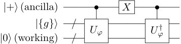 Figure 1
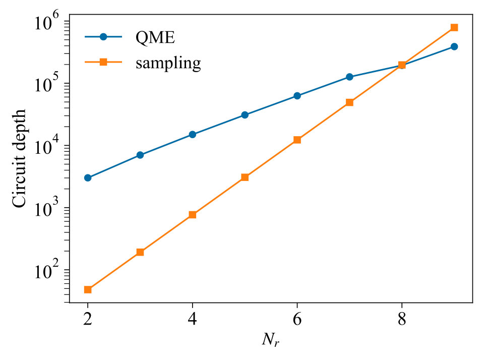 Figure 2
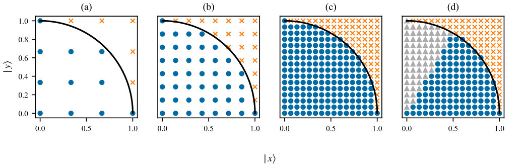 Figure 3
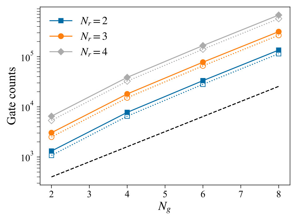 Figure 4
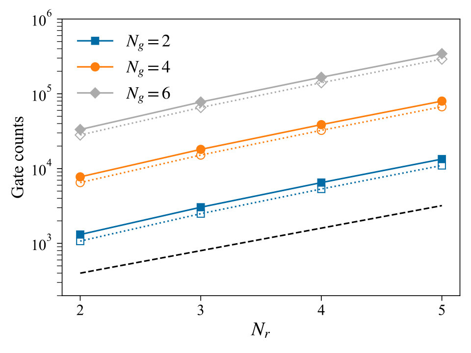 Figure 5
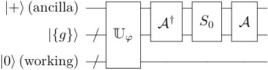 Figure 6
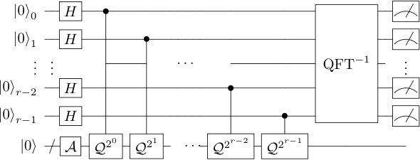 Figure 7
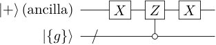 Figure 8
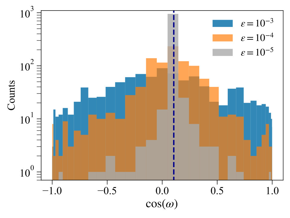 Figure 9
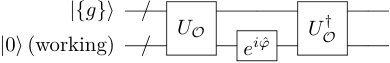 Figure 10
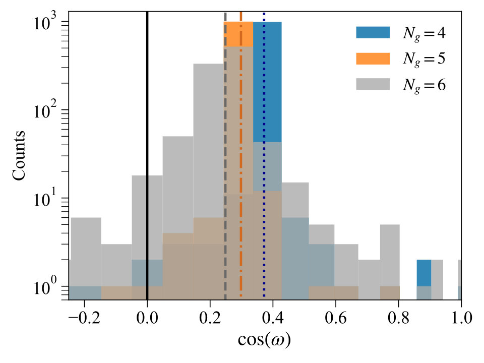 Figure 11
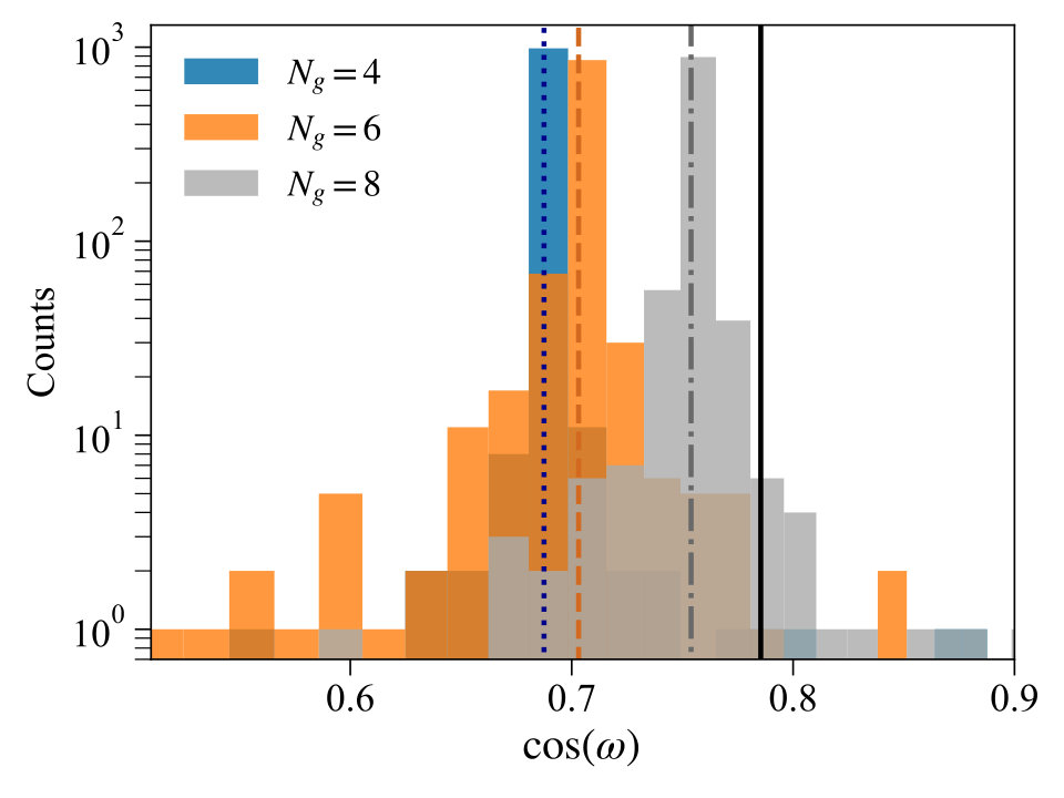 Figure 12
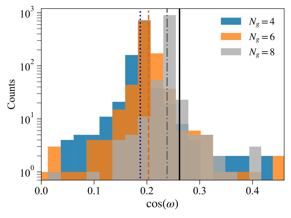 Figure 13
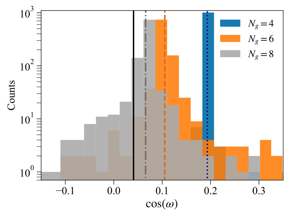 Figure 14
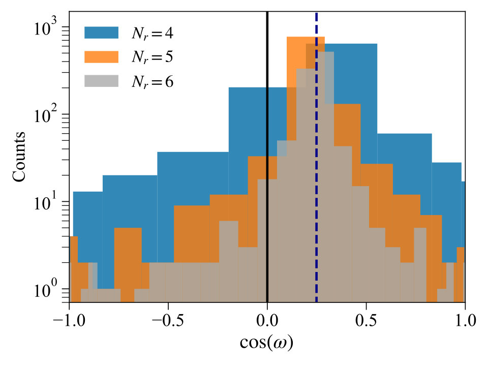 Figure 15
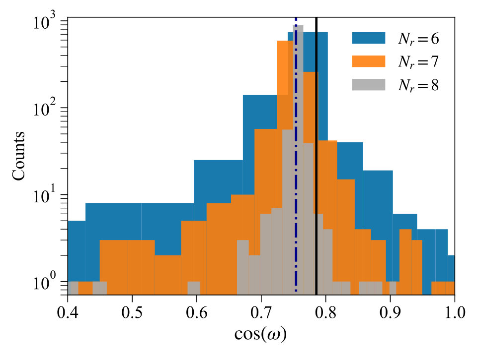 Figure 16
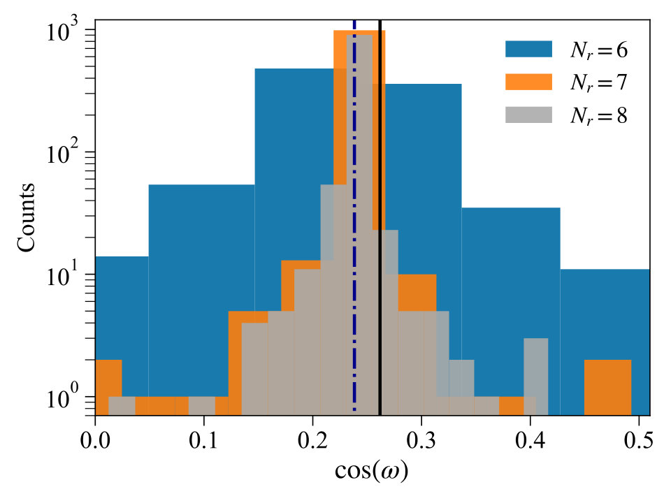 Figure 17
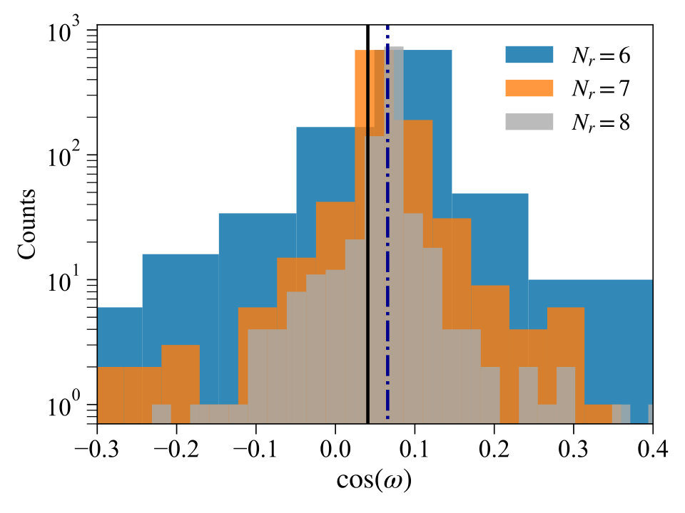 Figure 18
Peer Reviews
No public reviews on file for this paper yet. If you reviewed it on a platform where reviews are public (OpenReview, ICLR, NeurIPS, ICML), you can paste yours below so the community can read it here.
Videos
No videos yet. Explain this paper in a talk, walkthrough, or lecture? Add one.
Quantum mean estimation for lattice field theory
Erik J. Gustafson
Fermi National Accelerator Laboratory, Batavia, Illinois, 60510, USA
Henry Lamm
Fermi National Accelerator Laboratory, Batavia, Illinois, 60510, USA
Judah Unmuth-Yockey
Fermi National Accelerator Laboratory, Batavia, Illinois, 60510, USA
Abstract
We demonstrate the quantum mean estimation algorithm on Euclidean lattice field theories. This shows a quadratic advantage over Monte Carlo methods which persists even in presence of a sign problem, and is insensitive to critical slowing down. The algorithm is used to compute with and without a sign problem, a toy U(1) gauge theory model, and the Ising model. The effect of -gate synthesis errors on a future fault-tolerant quantum computer is investigated.
††preprint: FERMILAB-PUB-23-095-QIS-T
I Introduction
Computations in lattice field theory (LFT) are typically framed within the formalism of statistical mechanics [1, 2, 3]. This is possible by analytically continuing the field theory from Minkowski to Euclidean spacetime, which transforms complex phases into probability weights. This changes the quantum path integral into a classical partition function, , which is a sum over all configurations of the degrees of freedom, , weighted by the lattice action, . Quantum expectation values of observables, , then transform into statistical averages
[TABLE]
Summing over all configurations is, in general, impractical. Instead, Monte Carlo methods sample a finite number, , of them with an error, , on scaling asymptotically like . Often, only a few thousand samples yield precision predictions for complex observables like hadronic form factors [4] or QCD contributions to the muon [5].
However, there are limitations. These include situations where there is a sign problem [6, 7], and critical slowing down [8]. The sign problem crops up at finite fermion density [9] and when simulating real-time dynamics [10]. Critical slowing down is a consequence of running Monte Carlo algorithms with updates that neglect long-distance correlations. Such a situation appears as one tries to approach the continuum limit or when studying topological observables [11]. In the case of the sign problem, the required scales exponentially in model parameters, and with critical slowing down it scales as a power. These obstacles have prompted new classical algorithms that attempt to address these issues including: cluster algorithms [12, 13], dual variables approaches [14, 15], tensor networks [16, 17], complexification [10], and density of states methods [18]. Despite these successes, it is unlikely that general solutions exist cf. [19].
Through quantum computers it is possible to avoid some of these limitations. This result comes fundamentally from the abilities of quantum computers to enumerate an exponential number of states via quantum superposition, and their capacity to generate entanglement. Notable quantum algorithms which harness these properties include the quantum Fourier transform [20, 21, 22], quantum phase estimation (QPE) [23, 24, 25, 26], and Hamiltonian simulation. This last class of algorithms could further allow for tremendous advances in simulating real-time dynamics for LFT [27, 28, 29, 30, 31, 32, 33, 34, 35, 36, 37, 38, 39, 40, 41, 42, 43, 44, 45, 46, 47, 48, 49, 50, 51, 52, 53, 54, 55, 56, 57, 58, 59, 60, 61, 62, 63, 64, 65, 66, 67, 68, 69, 70, 71, 72, 73, 44, 68, 74, 75, 76, 77, 41, 78, 79, 80, 81, 82, 83]. Investigation of quantum algorithms have also lead to faster classical algorithms [84, 85].
Another quantum algorithm relevant specifically to this work is quantum mean estimation (QME) [86, 87, 88]. Quantum mean estimation is capable of quadratically reducing the asymptotic scaling of to . It achieves this using QPE, and by using superposition to incorporate a full probability distribution into calculations of . It has been developed for boolean variables, positive bounded real variables [89, 90], bounded real variables [87], and unbounded real variables [91, 86, 88].
In this article, we will demonstrate how and when QME can be used to improve classical LFT calculations that use Monte Carlo sampling. In Sec. II, we detail how to use QME on classical statistical models, and provide circuits to construct the QME algorithm. In Sec. III, we provide numerical results including circumstances with sign problems, and investigate the effects of noise. In Sec. IV, we compare traditional sampling methods to the QME algorithm. We conclude with a discussion and directions for future work in Sec. V.
II Quantum Mean Estimation
In this section, we will demonstrate how a quantum computer using QME can provide an estimate of with fixed precision and quadratically fewer resources than traditional sampling using the method of Ref. [87].
II.1 Overview of QME
Estimating on a quantum computer uses QPE as a subroutine. By encoding into the phases of states and running QPE on a judiciously chosen unitary and starting state, a phase is returned approximating the mean. Alternatively, the mean can be stored as the amplitude of some target state. This amplitude can be approximated and returned—again using QPE—using quantum amplitude estimation [92, 90, 89, 91, 88].
Following Ref. [87], for a given unitary—or phase oracle—in diagonal form,
[TABLE]
QME returns
[TABLE]
where is a generic initial state.111One can also estimate , but we focus on the real part. For appropriate s, one can calculate averages of real numbers . We provide here a method to construct through qubit arithmetic, by computing the appropriate into a register, applying a phase based on that register’s value, and then uncomputing the phase register back to . The computation of the is done by a new oracle, which for a given configuration, , places the state into a separate register. In terms of states and operators,
[TABLE]
The new “working” register stores the value of the appropriate phases to apply to each configuration. From that state, the proper phase can be applied via
[TABLE]
and the working register can be uncomputed,
[TABLE]
This entire circuit can be captured by a single unitary , as seen in Fig. 1.
Using QME corresponds to recasting Eq. (1) in the form of Eq. (II.1). The relevant identification is to see that the product . This identification in turn allows for flexibility in defining and the phases . Since we can identify in Eq. (II.1) as the probability for configuration used in the average, a natural correspondence is given by as well as , which can be used to define . However, one is allowed the freedom to reweigh parts of the observables into the weights, and vice versa, to optimize. By rescaling, this method can compute averages in any finite range.
To actually compute Eq. (II.1) requires preparing a state , and the use of QPE with . We will present two separate implementations of QME using two different . One directly prepares the Boltzmann weights, and the other shifts the difficulties of preparing such states into the computation of observables through reweighting.
II.2 Using state preparation
We can use any state-preparation method, whether it be through efficient classical methods [93], black-box methods [94, 95, 96], using the quantum singular value transform [97], or with state search [98] to construct an appropriate . Here, we prepare using arithmetical oracles such that . We will denote this state preparation method as .
To prepare a quantum state with the desired probability distribution, let be the weights of the system, and with the total number of configurations. We can prepare a maximal superposition over all configurations, along with an ancilla in the state :
[TABLE]
Next, we apply a controlled- with using the procedure from Sec. II.1,
[TABLE]
The phases used in state preparation are denoted with , and those used in encoding observables with , since both use the same phase oracle. After applying a Hadamard to the ancilla we can rewrite the whole state as,
[TABLE]
where is the desired state,
[TABLE]
and is an orthogonal state,
[TABLE]
contains the target probability distribution; however, needs to be removed. We use fixed-point oblivious amplitude amplification [99, 100, 101], which requires a lower-bound on the amplitude, to isolate the zero-ancilla state. A crude lower bound is given by assuming every comes with the smallest possible weight, then,
[TABLE]
We find that , and we can use as a lower bound for amplitude amplification. Asymptotically the algorithm will take amount of time to achieve a desired accuracy [99]. Deriving a tighter lower bound would reduce the algorithmic time; however, since the actual amplitude is , at best we can expect time. The algorithm requires no conditional measurements, or “repeat-until-success” steps, and is captured by a unitary matrix. After amplitude amplification we end with the desired state,
[TABLE]
The QME algorithm requires an ancilla in the state , so after applying a Hadamard gate, the initial state is
[TABLE]
Having prepared , we can use QPE to perform the mean estimation, but this state preparation is potentially expensive; therefore, we discuss an alternative approach.
II.3 Using reweighting
Previously, we discussed how there exists freedom in associating the product to and . The choices made determine the state preparation and the specific means computed. This reweighting [102] can be understood by introducing into Eq. (1) a second probability distribution :
[TABLE]
where and is a necessary reweighting factor. So instead of with the distribution , we can construct a different one by shuffling part of the distribution into the observable, and then computing the ratio of two means. One nice choice is the uniform distribution which can be prepared by . With two different state preparation methods described, we now discuss the role of QPE.
II.4 Quantum phase estimation
The QPE algorithm returns an estimate of a phase of an eigenvector for a unitary such that . Thus, QPE expects an input state, or a state preparation method , a unitary matrix whose eigenvalues are of interest, and a result register of qubits prepared in a maximal superposition. It then returns the best, approximate phase with a probability [20, 26].
We can see the effect of the input state not being an eigenstate of by inspecting its spectral decomposition,
[TABLE]
For a generic state ,
[TABLE]
and QPE operating on returns angle for each eigenstate into the result register in superposition with probability . The accuracy of the returned phase and how likely that phase is to be measured, is specified by . The possible phase values are restricted to the possible binary fractions expressible by qubits.
II.5 Synthesis of parts
Here we relate to to see how QME emerges from QPE. In Secs. II.2 and II.3 we discussed two methods. With those in mind, we will now construct used in QME. The unitary is given by the product with a phase oracle, , and the operator, . The form of is: , with . The circuit for can be seen in Fig. 2, and consists of applying a minus sign to the “all zeros” state. The phase oracle of Ref. [87] has two terms,
[TABLE]
and is responsible for applying the phases encoding onto the states. The oracle is described in Sec. II.1. The circuit for can be seen in Fig. 3, and with it can be completely defined. The circuit for can be seen in Fig. 4. The entire circuit for QPE—and through it QME—can be seen in Fig. 5.
With the relationship between and established the desired mean must come about from an eigenvalue of . To see this, let us revisit Eq. (II.1), and define the angle along with through,
[TABLE]
Written in this form we see that Eq. (19) computes the average value of cosine. Now, consider the initial state . While not an eigenstate of , it is a simple linear combination of eigenstates of (see Ref. [87]),
[TABLE]
with . Since is constructed from eigenvectors of , applying QPE to returns either of the two phases associated with those states, or , with equal probability. Then by taking the cosine of the output angle—which is insensitive to or —we recover the average in Eq. (19).
To summarize,
Using a qubit encoding of , construct . This can either be done by making a state with the correct probability distribution as in Sec. II.2, or by reweighting as in Sec. II.3.
- 2)
Construct :
- –
Construct . This is model- and observable-dependent but consists of qubit arithmetic. Define the phases, , as needed.
- –
Construct from and using Fig. 1.
- –
Construct from using Fig. 3.
- 3)
Construct from , , and using Fig. 4.
- 4)
Perform QPE with and as in Fig. 5. The output is an estimated angle, , where .
With the method now explained, we proceed with some examples to help solidify each step above.
III Applications
We consider several numerical examples: computing with and without negative weights, a toy U(1) gauge theory, and the two-dimensional Ising model. Then, a general QME is described for lattice gauge theories. Finally, how -gate synthesis errors affect QME is discussed. All of the numerical results in this section were performed on the IBM Qiskit QASM simulator using 1024 shots.
III.1 with and without a sign problem
In the Monte Carlo estimate of , one randomly chooses points, in the - plane—which we assume to be a grid (see Fig. 6)—such that . A quarter circle in that plane has an area of , while the square has area one. Then we expect that on average the fraction of points that fall within the boundary of the circle is . We can decide this for each - pair if , and by counting the number of points that fall inside the circle we can compute .
To compute using a quantum computer, parameterize and using qubits: , , which creates an equal superposition of all possible - pairs. The () coordinate is defined as the integer representation of the bit-string associated with () normalized by . For example, the state when normalized corresponds to . With the addition of a single ancilla qubit prepared in the state, this preparation of the - coordinates constitutes .
To construct , we need to define the phase oracle, . Let us consider a statistical mechanics average:
[TABLE]
where is the Heaviside function, , and . Going forward we will give the and dependence once, but omit it afterward. We approximate this integral using a grid of points,
[TABLE]
where , i.e. the number of points in the grid.
The phases for are then defined as , with the two cases: when , and when . Since the - coordinates are in superposition we can demonstrate the action of on a single pair without loss of generality. We will use quantum arithmetic gates [103, 104] specifically an addition gate, , and a multiplication gate, . Further we require a comparator , that returns a boolean variable [105]. First we add and into two registers,
[TABLE]
Then, we multiply the registers together,
[TABLE]
and add the products together
[TABLE]
Finally, we compare to a register,
[TABLE]
where the comparison register is either zero or one. This defines . Using this register, a phase can be applied which gives if the comparison bit is zero, or if it is one. The working registers can be uncomputed, defining the entire unitary . With defined, is defined, and with , is defined, and QPE can be performed.
Histograms showing counts of bit-strings using different and are in Figs. 7, and 8, respectively. Along with the histograms are lines for the finite-grid ratios of inner-circle points to total points, as well the exact value of . In Fig. 7, we see an increase in at fixed , leading towards , with a constant bin width at no less than an exponential rate. In practice, one could extrapolate the measured value as a function of with potentially fewer resources than a single fine grid might require. In Fig. 8, we see varying while keeping yields a most likely value at the finite-grid ratio, and the bin width diminishes as . Thus, larger improves accuracy, while larger improves precision.
We can include a sign problem by weighing locations in the quarter circle using positive and negative weights separated at which corresponds to (See Fig. 6 (d)). When , the weight is , and when , the weight is . This corresponds to the integral
[TABLE]
To estimate from Eq. (27) we must modify to also check if . We compute and as before, and using a division oracle calculate which is then compared using with . We then apply a phase based on the compare register. Therefore, with a sign problem there are two deciding qubits, and , which indicate if the point is inside the circle and , respectively. From their values a phase is imparted, with . With the working register arithmetic outlined above, , , and are defined.
Analogous histograms to the case of without a sign problem can be seen in Figs. 9 and 10. We see in Fig. 9 as is varied with fixed , the most likely value moves towards for larger values of . Likewise, in Fig. 10 as is increased we see the distribution narrows around the finite-grid ratio. For QME this problem is as computationally difficult as without a sign problem. One should note that the nonlinear transform from the measured to results in non-constant bin width. This is acutely important for sign problems and reweighting when means are often near zero, where the bins are largest. Thus rescaling the result register to optimize bin locations could be valuable for reducing costs.
III.2 U(1) gauge theory toy model
We introduce a toy model resembling the Villian [106, 107] approximation of a two-dimensional, Euclidean U(1) gauge theory, and the calculation of the Wilson loop. This has been used to investigate classical methods for ameliorating the sign problem [108]. We aim to calculate
[TABLE]
Here, controls the degree of oscillations in the integrand and can be any real number. The value of is
[TABLE]
We again approximate and by a grid and .
State preparation is given by . We will encapsulate inside the phases and define . Designing the circuit for computing the phases requires floating-point arithmetic, which we will not elaborate upon, but will assume exist. With the ability to create , we can apply to the phase register and extract the phase. After uncomputing the phase register, this procedure defines and .
Results of these circuits for are shown in Figs. 11 and 12. In Fig. 11 we see that as is increased the distribution narrows around the exact value. Figure 12 shows the drift of the most likely value of towards the exact value of as increases at fixed .
Having given circuits and explained QME for a variety of toy and demonstrative models, we now turn to an archetypal LFT, the Ising model.
III.3 The Ising model
We consider a two-dimensional Ising model on a Euclidean lattice with periodic boundary conditions and spatial and temporal extents of and . The action is
[TABLE]
where sums over nearest-neighbor pairs, is a lattice spin taking values , and is a coupling constant commonly identified as an inverse temperature. We can rewrite this as a sum over binary values, , using . Then
[TABLE]
As an observable, we will compute the square of the magnetization density
[TABLE]
which is bounded between zero and one.
On the quantum computer each qubit in the system is associated with a spin on the lattice. To prepare the system, we put every qubit into the state, . This generates all spin configurations in superposition. By appending one ancilla prepared in the state we have the state preparation circuit , but must calculate a ratio of observables (see Sec. II.3).
Just as in the example, we require a phase oracle. We will focus on a single spin configuration without loss of generality. To compute the magnetization, we must sum the bit-string. We do this by first summing every even-odd spin together in parallel. We can then add the results of the first step again in even-odd pairs. Repeating this we can compute the sum in steps. The result of these sums is . By multiplying by two, dividing by the volume, and shifting by one we arrive at the magnetization density. We can add this number to zero, and multiply the two registers to obtain .
To compute the action, we already have the term containing . To compute the nearest-neighbor interaction we can again compute the product of disjoint pairs of spins in each of the two directions in parallel, and sum the resulting collection of products. This can be done in steps, resulting in a register . Multiplying by the appropriate factors and subtracting we can form the register . Then using exponentiation, multiplication, and taking the arccosine we arrive at . This defines for the numerator. for the denominator can be calculated similarly without the factor of . Now by applying we can extract the phase, then uncompute the phase register. These steps define the unitary , and hence , in QPE.
In Figs. 13 and 14 we see histograms of when varying and respectively, for the one-dimensional, classical Ising chain at . As is increased for fixed , the mean tends towards the infinite-volume value. Likewise, with fixed and increased, estimates converge to the exact finite-volume value.
Fig. 14 demonstrates a desirable feature that results from 1) the bin-width providing a 100% confidence interval of error, and 2) the maximal bin changing location. That is that the ideal result must lie in the overlap between distributions. Therefore, the overlap between bins of different can estimate the mean more precisely than any single alone. This could be used to engineer sets of that maximize information gained. In Fig. 14 we see a sliver of overlap between the and maximal bins, which the exact answer must lie within. Fig. 11 provides another example. Having now seen QME used with simple examples, as well as the formulation and execution on a bona fide LFT, we now give the formulation of QME for a generic lattice gauge theory.
III.4 Generic lattice gauge theory
Take a dimensional lattice with and periodic boundary conditions. We consider the action
[TABLE]
where is a plaquette, is a gauge group element, and the sums are over lattice sites and the two directions and respectively .
Prepare a qubit register for each gauge link, . Let the operator prepare a maximal superposition of all possible gauge link states, analogous to the Hadamard gate,
[TABLE]
where is the size of the local state space. Then for state preparation we can apply for every link register,
[TABLE]
This creates a superposition of all field configurations with equal probability. We then append an ancilla qubit . This constructs . For we follow Sec. II.2 with . When encoding observables one sets in . With these prescriptions of the phases, the operators for QME of lattice gauge theory are defined. In the next section we will study the effects of noise on QME.
III.5 The effects of noise
On a fault-tolerant quantum computer the gates are approximated with an infidelity by interleaved and gates [109, 110, 111, 112, 113, 26, 114, 115]. While one can derive a string of and gates that approximates any gate, implementing this string and classically simulating it drastically extends the length of a quantum circuit, and becomes a computationally intensive problem. Instead, to study the effects of nonzero , we approximate each gate,
[TABLE]
The parameter approximates the infidelity in quantum computations, and drives coherent angle-dependent drift in the gates. We tested variations on Eq. (36) by sending in and found negligible effects.
For a test case we consider the model from Sec. III.2. Using we run the QME circuit for various . This calculation requires synthesizing gates. Fig. 15 shows the histogram of the average returned from QME. For a statistically clear signal for the most likely value consistent with the ideal value appears with .
In context, this indicates there is a threshold for a given set of shots below which better synthesis of provides no benefit at fixed and . Exact rotation gates are unnecessary, and imprecise rotation gates can give sufficient accuracy and precision. This is analogous to precision LFT calculations where half-precision floating point numbers are used to accelerate calculations [116, 117, 118, 119]. Heuristically, the threshold is .
IV Quantum advantage
To appreciate the advantage provided by the QME algorithm, consider . At this stage, traditional sampling methods could be applied, and measuring provides a single configuration. By iterating this procedure one collects an ensemble of configurations from which averages can be taken. We expect , but is precisely the number of times is run. In this sense we can see as the quantum mechanical analog to having access to the partition function through, say, brute-force calculation.
Now, without loss of generality, take to be a power of two, , implying . For the QME algorithm, we want the same precision of . Using QME we see this requires qubits. Looking at Fig. 5, QPE executes a total of times. Since appears in times, is similarly called times. Thus we see the number of times is needed in the QME algorithm () is quadratically less compared to the traditional sampling method (). Therefore rather than using the prepared state to sample and calculate expectation values, it is advantageous to pass the quantum state into the QME algorithm to avoid greater calls to the state preparation algorithm overall, while maintaining the same precision.
This increased efficiency in calls to is seen in Fig. 16, where QME is compared with the traditional sampling method to calculate for and varying . Both the QME and sampling circuits are decomposed under the same basis gates. We see the overhead for QME is large, however for a fixed accuracy, the scaling of QME is superior to sampling. The ratio between the sampling and QME slopes is , approaching the asymptotic quadratic value. The sampling circuit depth is computed using the circuit depth for , multiplied by the number of samples required to achieve a precision of assuming the error converges like . After , QME surpasses the traditional sampling method in efficiency.
What about in the case of a sign problem, or an exponentially small value to calculate? This is relevant in the case of . Consider the case where the degrees of freedom of the model are binary variables themselves. Now the prefactor in Sec. II.2 can be rewritten as
[TABLE]
where is the free energy density, . This same factor appears in the final ratio when computing using Sec. II.3 as well. We see that this ratio depends exponentially on the number of qubits used in the system—note that is always less than here, since the Boltzmann weights will always be less than or equal to one, and when all Boltzmann weights are one. Therefore, to compute a number as small as using QME will require qubits in the result register, which will entail calls to . Notice this is still quadratically faster than traditional sampling, since naively
[TABLE]
Therefore even in the case of a sign problem or an exponentially small signal, the QME algorithm is superior.
For many state preparation methods, QME depends exponentially on the system volume. This is paid either in the amplitude amplification step, or in the precision of calculating the mean during QPE. This dependence comes from producing the full probability distribution; however, one can instead approximate the distribution. This is relevant to the case of classical sampling algorithms. Using pseudo-random number generators, these algorithms sample from approximate probability distributions. Since classical algorithms can be ported onto a quantum computer [120, 26], these distributions can be realized by an circuit. Even still, QME calls quadratically fewer times than would be required by sampling, and so calculations of are accelerated—at least asymptotically. Moreover, should classical algorithms improve in the future, QME can take those state preparation methods and use them, along with a further advantage.
In light of this discussion, we can study the resource costs for QME. We do this for the example of computing without a sign problem. In Figs. 17 and 18 we see the total and CNOT gate counts as a function of , and , respectively. In both cases we see an exponential dependence. This can be understood as follows: an increase in exponentially increases the precision of the result in QPE. Likewise, as we increase the grid fineness increases, and the accuracy improves exponentially. The growth in gate count is therefore a reflection of the improvement in the accuracy and precision of the result with growth in both and .
V Conclusion
We have shown how QME can estimate Euclidean LFT observables. The method relies on QPE and provides a quadratic speed-up over traditional methods. The possible improved scaling in the calculation of expectation values is tantalizing. While the gate costs seem to require fault-tolerant quantum computers, further optimizations can reduce those costs. Possible directions include improving QPE [121, 25, 122] over the version used here, or advancements in encoding phases into the result register in other formats, e.g. floating point. Crucially, quantum state preparation of the probability distribution dominates the resource estimate. However when using amplitude amplification, it is still quadratically faster than classically constructing the distribution. Further reductions may occur by fitting the measured phase distribution instead of taking only the most likely value.
Quantum mean estimation also provides an alternative perspective on sampling. When calculating expectation values, the quantum system must be prepared, measured, and re-prepared. Similarly, classical sampling algorithms follow this pattern, albeit obfuscated. Quantum mean estimation instead embeds the preparation and measurement actions into the quantum algorithm itself via quantum superposition. The average is returned with high probability, meaning, the only sampling necessary is used to distinguish the correct bit-string from others. Moreover this speed-up persists even for sign problems and near criticality. This advantage is appealing for LFT practitioners, where these issues are prohibitive. Conversely, the speed-up provided by QME is only polynomial, and hence, the prefactors will dictate its utility. Applying the algorithm on real quantum hardware with simple examples will elucidate its long-term scaling and practicality.
Acknowledgements.
The authors thank Prasanth Shyamsundar for reading drafts of the manuscript, and Michael Wagman for stimulating discussions. This work is supported by the Department of Energy through the Fermilab QuantiSED program in the area of “Intersections of QIS and Theoretical Particle Physics”. Fermilab is operated by Fermi Research Alliance, LLC under contract number DE-AC02-07CH11359 with the United States Department of Energy.
The reference list from the paper itself. Each links out to its DOI / PubMed record.
- 1Montvay and Münster [1994] I. Montvay and G. Münster, Quantum Fields on a Lattice , Cambridge Monographs on Mathematical Physics (Cambridge University Press, 1994). · doi ↗
- 2Gattringer and Lang [2010] C. Gattringer and C. B. Lang, Quantum Chromodynamics on the Lattice , Lecture Notes in Physics (Springer Berlin, Heidelberg, 2010). · doi ↗
- 3Kogut [1979] J. B. Kogut, An introduction to lattice gauge theory and spin systems, Rev. Mod. Phys. 51 , 659 (1979) . · doi ↗
- 4Bazavov et al. [2022] A. Bazavov et al. (Fermilab Lattice, MILC, Fermilab Lattice, MILC), Semileptonic form factors for B → D ∗ ℓ ν → 𝐵 superscript 𝐷 ℓ 𝜈 B\rightarrow D^{*}\ell\nu at nonzero recoil from 2 + 1 2 1 2+1 -flavor lattice QCD: Fermilab Lattice and MILC Collaborations, Eur. Phys. J. C 82 , 1141 (2022) , [Erratum: Eur.Phys.J.C 83, 21 (2023)], ar Xiv:2105.14019 [hep-lat] . · doi ↗
- 5Borsanyi et al. [2021] S. Borsanyi et al. , Leading hadronic contribution to the muon magnetic moment from lattice QCD, Nature 593 , 51 (2021) , ar Xiv:2002.12347 [hep-lat] . · doi ↗
- 6de Forcrand [2009] P. de Forcrand, Simulating QCD at finite density, Po S LAT 2009 , 010 (2009) , ar Xiv:1005.0539 [hep-lat] . · doi ↗
- 7Tripolt et al. [2019] R.-A. Tripolt, P. Gubler, M. Ulybyshev, and L. Von Smekal, Numerical analytic continuation of Euclidean data, Comput. Phys. Commun. 237 , 129 (2019) , ar Xiv:1801.10348 [hep-ph] . · doi ↗
- 8Schaefer et al. [2011] S. Schaefer, R. Sommer, and F. Virotta (ALPHA), Critical slowing down and error analysis in lattice QCD simulations, Nucl. Phys. B 845 , 93 (2011) , ar Xiv:1009.5228 [hep-lat] . · doi ↗