A multivariate Riesz basis of ReLU neural networks
Cornelia Schneider, Jan Vyb\'iral

TL;DR
This paper proves that a certain system of piecewise linear functions forms a Riesz basis for multivariate $L_2$ spaces, which can be efficiently represented by neural networks and is dimension-independent.
Contribution
It provides an alternative proof of the Riesz basis property and generalizes the system to higher dimensions without tensor products, facilitating neural network representations.
Findings
The system forms a Riesz basis of $L_2([0,1])$.
The basis generalizes to higher dimensions $d>1$.
Riesz constants are independent of the dimension $d$.
Abstract
We consider the trigonometric-like system of piecewise linear functions introduced recently by Daubechies, DeVore, Foucart, Hanin, and Petrova. We provide an alternative proof that this system forms a Riesz basis of based on the Gershgorin theorem. We also generalize this system to higher dimensions by a construction, which avoids using (tensor) products. As a consequence, the functions from the new Riesz basis of can be easily represented by neural networks. Moreover, the Riesz constants of this system are independent of , making it an attractive building block regarding future multivariate analysis of neural networks.
Click any figure to enlarge with its caption.
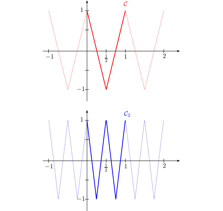 Figure 1
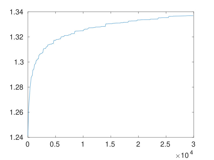 Figure 2
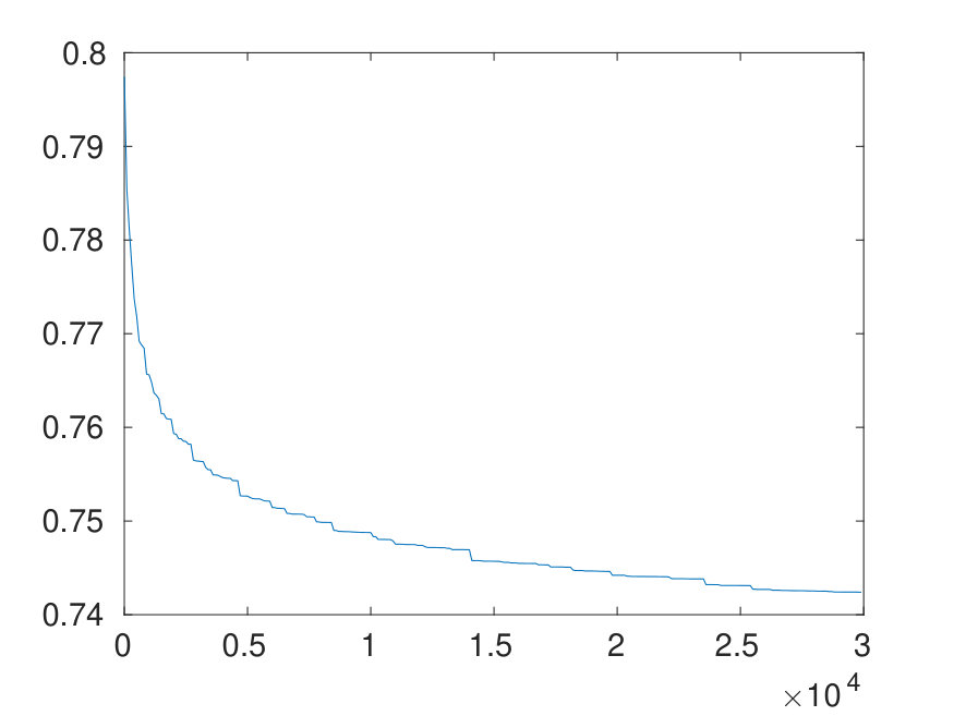 Figure 3
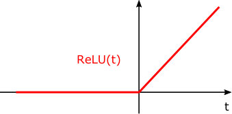 Figure 4
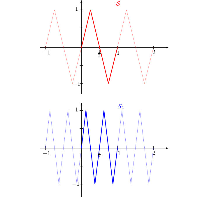 Figure 5
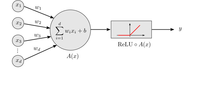 Figure 6
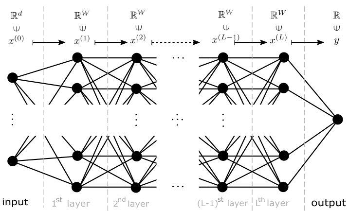 Figure 7
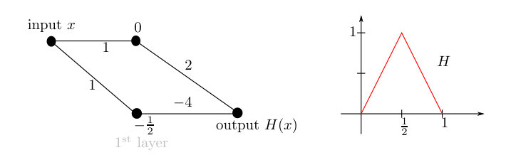 Figure 8
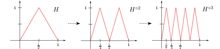 Figure 9
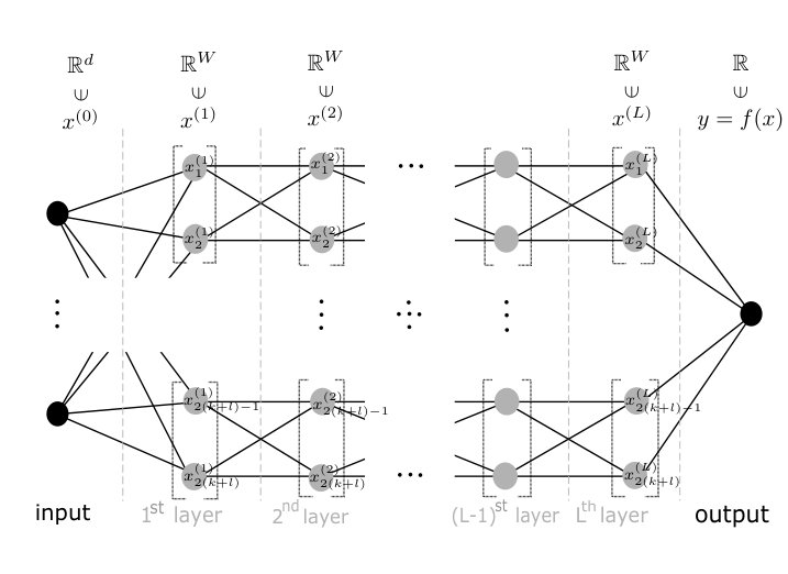 Figure 10
Peer Reviews
No public reviews on file for this paper yet. If you reviewed it on a platform where reviews are public (OpenReview, ICLR, NeurIPS, ICML), you can paste yours below so the community can read it here.
Videos
No videos yet. Explain this paper in a talk, walkthrough, or lecture? Add one.
Taxonomy
TopicsModel Reduction and Neural Networks · Computational Physics and Python Applications · Neural Networks and Applications
A multivariate Riesz basis of ReLU neural networks
Cornelia Schneider111Friedrich-Alexander Universität Erlangen, Applied Mathematics III, Cauerstr. 11, 91058 Erlangen, Germany. Email: [email protected] and Jan Vybíral222Department of Mathematics, Faculty of Nuclear Sciences and Physical Engineering, Czech Technical University, Trojanova 13, 12000 Praha, Czech Republic. Email: [email protected]. The work of this author has been supported by the grant P202/23/04720S of the Grant Agency of the Czech Republic
Abstract
We consider the trigonometric-like system of piecewise linear functions introduced recently by Daubechies, DeVore, Foucart, Hanin, and Petrova. We provide an alternative proof that this system forms a Riesz basis of based on the Gershgorin theorem. We also generalize this system to higher dimensions by a construction, which avoids using (tensor) products. As a consequence, the functions from the new Riesz basis of can be easily represented by neural networks. Moreover, the Riesz constants of this system are independent of , making it an attractive building block regarding future multivariate analysis of neural networks.
Key Words: Riesz basis, Rectified Linear Unit (ReLU), artificial neural networks, Euler product, Möbius function
MSC2020 Math Subject Classifications: 68T07, 42C15, 11A25.
1 Introduction
The last decades observed a tremendous success of artificial neural networks in many machine learning tasks, including computer vision [16], speech recognition [11], natural language processing [24], or games solutions [17, 21] to name just few. Despite their wide use, many of their properties are not fully understood and many aspects of their great practical performance lack a rigorous explanation. Without any doubt, a deeper insight into the theory of artificial neural networks could boost their applicability even further.
In the last decade, a growing number of authors investigated why the deep neural networks with a higher number of hidden layers approximate many interesting functions more efficiently than the shallow neural networks (with only one hidden layer) using the same number of parameters. We refer to [1, 7, 8, 10, 12, 18, 22, 25] for a number of mathematically rigorous results in this direction.
One of the astonishing properties of artificial neural networks is, that they can approximate extremely well also functions of many variables, which often allows to avoid the curse of dimensionality [3, 9, 19]. The aim of this work is to shed new light on the effectiveness of artificial neural networks for the approximation of multivariate functions by constructing a new system of functions, which forms a Riesz basis of for every .
To state the result, we first recall the notion of a Riesz basis (which, in turn, is a generalization of an orthonormal system and of an orthonormal basis, cf. [6]).
Definition 1.1**.**
Let be a real Hilbert space. The (finite or infinite) sequence is called a Riesz sequence if there are two constants such that
[TABLE]
for every real square summable sequence . If the closed span of is the whole space , then we call it a Riesz basis.
The system, which we study in this paper, is a trigonometric-like basis, where instead of and functions we use their piecewise linear counterparts and , which are defined as follows (cf. Figure 1).
Definition 1.2**.**
For , we define
[TABLE]
and
[TABLE] 2. 2.
For , we extend this definition periodically, i.e. and 3. 3.
If and , we put and
These functions were introduced and studied in [7], where it was shown that the system
[TABLE]
forms a Riesz basis of with the constants and Let us note that the factor in (2) is simply a normalization factor, which ensures that all the elements of have unit norm in . The proof given in [7] is implicitly inspired by the method of analysis and synthesis operators, respectively, used in the frame theory, cf. [13]. It is one of the aims of our paper (cf. Theorem 2.2) to provide an alternative proof, which first reduces (1) to the study of spectral properties of the Gram matrix of . The result then follows from the Gershgorin circle theorem and some elementary number theory (including Euler products and a certain Ramanujan’s formula).
The main advantage of (2) in contrast to the standard trigonometric system is, that its elements can be easily identified by artificial neural networks with the REctified Linear Unit (ReLU) activation function.
Let us recall, that if , then the ReLU function is defined as , cf. Figure 2. On vectors, it acts component-wise
[TABLE]
If and are integer parameters, then we denote by the real-valued functions which can be represented by a neural network of width and depth , see Definition 4.1 for a precise formulation. Then [7, Theorem 6.2] shows that and (restricted to ) lie in for an arbitrary and of the asymptotic order
The main aim of our work is to generalize the results of [7] to the multivariate case. There are two crucial issues which prevent us from simply taking the tensor products of the functions in . First, the product function can only be approximated by the neural networks and, second, the ratio of the Riesz constants and gets exponentially large when grows.
We propose a surprisingly simple and effective solution to these challenges. We show that (cf. Theorem 3.3) the multivariate analogue of
[TABLE]
forms a Riesz basis of for every with the same constants and as in the univariate case. Here, \alpha\mathrel{\makebox[7.7778pt]{\raisebox{0.3pt}{\clipbox{.30pt{} .30pt}{+}}\makebox[7.7778pt]{>}}}0 means that the first non-zero entry of is positive. Finally, we show in Section 4 that the functions from (3) can be exactly reproduced by the neural networks of width and depth in essentially the same way as in the univariate case, i.e., there is virtually no price to pay when grows.
2 Univariate case
It was observed in [7, Section 6], that the system of piecewise linear functions
[TABLE]
on one hand shares some nice properties with the trigonometric system and on the other hand can be easily reproduced by artificial neural networks with the activation function. The aim of this section is to essentially reprove Proposition 6.1 of [7], which states that this system is a Riesz basis of , the space of square integrable functions with mean zero.
Although our proof shares some technical details with [7], its main structure is different: In particular, we reduce the problem to spectral properties of the corresponding Gram matrix and then apply the Gershgorin circle theorem. Interestingly, by using some elementary number theory, we are able to completely characterize the inner products of the and/or functions. In contrast to [7], we complement (4) by adding the constant function, which is orthogonal to all functions from (4).
We denote by the greatest common divisor of and and by the standard inner product in
Lemma 2.1**.**
Let Then
; 2. 2.
* if is odd and is even (or vice versa), i.e., if the prime factorizations of and contain a different power of 2;* 3. 3.
If and are both odd, then
[TABLE]
Here, the sign of is negative if, and only if, is even. 4. 4.
In particular, we get for all .
Proof.
We transfer the proof to the Fourier side by exploiting the decomposition of and into Fourier series, cf. [7, page 166]. Let
[TABLE]
Then a standard calculation reveals that
[TABLE]
where
[TABLE]
Using (5), we immediately obtain that . Furthermore,
[TABLE]
where if and zero otherwise. To simplify (7), we have to find for fixed all such that . First, we observe that if the prime factorizations of and contain a different power of two, then also and have a different power of two in their prime factorizations and therefore they differ for all . Consequently, (7) shows that .
If the prime factorizations of and contain the same power of two, then and are both odd. We denote and note that and are coprime, i.e., that their greatest common divisor is one. We then look for all pairs , which solve the equation
[TABLE]
All the solutions are obtained in the form
[TABLE]
We insert (8) into (7) and conclude that
[TABLE]
The calculation of can be performed in a very similar way, one only needs to take care about the sign of the inner product. In particular, instead of (7) we obtain
[TABLE]
where if, and only if, is odd. Therefore, the sign is negative if, and only if, even. ∎
Next, we combine Lemma 2.1 with the Gershgorin circle theorem and provide an alternative proof of [7, Theorem 6.2], which we restate as follows.
Theorem 2.2**.**
The system is a Riesz basis of .
Before we come to the proof, several remarks seem to be in order.
Remark 2.3**.**
We will actually show, that the Riesz constants of the -normalized system can be chosen as and 2. 2.
We divide the proof of Theorem 2.2 into several steps. In the first two steps, we show that the truncated system forms a Riesz sequence (i.e., that it satisfies (1)) with and being independent of . The first step reduces this question to spectral properties of the Gram matrix of and in the second step we apply the Gershgorin theorem to bound this spectrum. The third step describes how we pass to the limit to deduce that is also a Riesz sequence. Finally, the fourth step shows that is also a basis, i.e., that its closed linear span is . 3. 3.
Our proof shows that the spectrum of the Gram matrix of (for arbitrary ) is contained in We leave it as an open problem to find out if these bounds are actually optimal. Supported by numerical evidence (see Figure 3 for details), our conjecture is that there is indeed some space for improvement.
Proof of Theorem 2.2: Step 1.
First we reformulate the definition of a (finite) Riesz sequence as an eigenvalue problem of its Gram matrix. This reformulation is rather straightforward and by no means new, see [15] or [26, Chapter 1.8]. Let be a real Hilbert space and let . Then, for every
[TABLE]
where with is the Gram matrix of . Therefore, (1) is equivalent to for every or simply to To show that this is indeed true for a given Gram matrix , we will use the Gershgorin circle theorem [14, Theorem 6.1.1], which states that
[TABLE]
Proof of Theorem 2.2: Step 2.
In this step, we show that forms a Riesz sequence for every with the Riesz constants independent on . By Lemma 2.1, its Gram matrix is a block matrix with three blocks. The first one is just a block corresponding to the constant function, the second and the third block are matrices of the inner products \big{(}3\langle\mathcal{C}_{i},\mathcal{C}_{j}\rangle\big{)}_{i,j=1}^{N} and \big{(}3\langle\mathcal{S}_{i},\mathcal{S}_{j}\rangle\big{)}_{i,j=1}^{N}, respectively, i.e.,
[TABLE]
We apply the Gershgorin theorem to . Therefore, we need to estimate the row sums of . For the first row we see that and for all .
Next we assume that is an odd number, i.e. that
[TABLE]
for some primes and integers . For the -th row (, corresponding to ) we conclude
[TABLE]
Every odd can be written as , where and is an odd integer, not divisible by any of , i.e., with . Observe that with this notation
[TABLE]
Therefore, we can use Lemma 2.1 and rewrite (9) as
[TABLE]
Next, we simplify the individual terms.
[TABLE]
and
[TABLE]
Therefore,
[TABLE]
where in the last step we used the following Euler product [23, Page 5] attributed already to Ramanujan
[TABLE]
Therefore, we get
[TABLE]
If is even it follows from Lemma 2.1, assertions 2. and 3., that the estimates above remain the same since only for ’s with the same power of in their prime factorization as , which then cancels out.
If we replace in (9) by (corresponding to the rows , of the Gram matrix), we obtain instead the estimate
[TABLE]
The term on the right hand side of (12) can be bounded by (10) as before and we again obtain
[TABLE]
By Gershgorin’s theorem, we deduce
Proof of Theorem 2.2: Step 3.
The third step of the proof of Theorem 2.2, i.e., the passage to the limit , is quite standard and straightforward (cf. [15] and [4, 5] for the so-called “projection method”) and is contained in the following lemma.
Lemma 2.4**.**
Let be a real Hilbert space and let be an infinite sequence. If is a Riesz sequence for every with Riesz constants and independent on , then is also a Riesz sequence with Riesz constants and .
Proof.
Let be a square-summable sequence. Since
[TABLE]
the partial sums of form a Cauchy sequence and therefore the series is convergent. Furthermore, by the triangle inequality
[TABLE]
Hence, we can take the limit in
[TABLE]
and the result follows. ∎
Proof of Theorem 2.2: Step 4.
As the last step, we show that is not only a Riesz sequence but also a Riesz basis, i.e., that its closed linear span is the whole space . We rely on the fact that the trigonometric system
[TABLE]
forms an orthonormal basis of . We show that every function from (14) lies in the closed linear span of and, therefore, the closed linear span of is contained in the closed linear span of
We start with the following lemma, which gives an explicit decomposition of and in . Its statement requires the notion of the Möbius function, which is defined for every positive integer as
[TABLE]
Lemma 2.5**.**
For every , let and , where is the constant from (6). Then
[TABLE]
and
[TABLE]
with the convergence being in .
Proof.
We first reformulate (5) as
[TABLE]
where and . Note, that (17) converges in .
We show that there is a unique bounded sequence , such that
[TABLE]
with the convergence in and that
[TABLE]
Using (17), we observe that (18) holds for bounded sequence if, and only if,
[TABLE]
We compare the coefficients of on both sides of (20) and observe that (20) is equivalent to the system of equations
[TABLE]
This system could be solved by using the Möbius inversion formula [23, p. 3], but one can also proceed directly. From we obtain and from we get . We show by induction that also for all . Let this be true for all integers smaller than . Then
[TABLE]
gives as well. Similarly, from we get for every prime .
Let now with odd primes . Then follows from
[TABLE]
The formula for a general , with distinct odd primes follows by induction. Observe that is divisible by all with . Hence
[TABLE]
We conclude, that for every odd square-free integer .
Finally, we show that for every positive odd integer , which is not square-free. Therefore, we assume that , where is an odd prime, is an odd integer not divisible by , and that the statement is true for all integers smaller than . We obtain
[TABLE]
If is square-free, then the first two terms in this sum have values and , respectively, and the others vanish by the induction assumption. If is not square-free, then all the terms vanish again by assumption. Finally, if the same argument applies leaving us with . We conclude that the sequence given by (19) indeed satisfies the system (21) which in turn gives (18).
Finally, (16) follows from (15) using the simple relation The factor results from the relation
[TABLE]
∎
3 Multivariate case
The main aim of this section is to generalize Theorem 2.2 to higher dimensions and to provide a Riesz basis of , which is easily expressed by artificial neural networks with activation function. The most natural approach would be to consider the tensor products of the functions from , i.e., a system of functions of the form etc. Indeed, it is quite easy to show that tensor products of elements of a Riesz sequence form again a Riesz sequence [2]. This approach is quite classical in analysis and there exist many multivariate bases and systems with a tensor product structure. Unfortunately, the Riesz constants of the tensor product system are in general given as products of the Riesz constants of the univariate Riesz sequences, cf. [2, Theorem 4.1]. Applying the tensor product construction to would therefore lead to an exponential dependence of the ratio of the Riesz constants on the dimension.
Furthermore, the tensor product approach does not fit really well to artificial neural networks. The reason is that it is surprisingly difficult to construct a neural network, which for two real inputs and outputs the product (or at least its approximation). In general, one first approximates the square function and then applies the formula We refer to [10, 20, 25] for details. Therefore, we are looking for another multivariate Riesz basis of piecewise affine functions, which can be constructed without the use of (tensor) products, but where inner products with fixed vectors in are allowed.
Before we state our results, we need some additional notation. If , we say that \alpha\mathrel{\makebox[7.7778pt]{\raisebox{0.3pt}{\clipbox{.30pt{} .30pt}{+}}\makebox[7.7778pt]{>}}}0 if the first non-zero entry of is positive. The multivariate analogue of is then defined simply as
[TABLE]
where we interpret the functions and as periodic functions on . Note that we need to restrict ourselves to indices \alpha\mathrel{\makebox[7.7778pt]{\raisebox{0.3pt}{\clipbox{.30pt{} .30pt}{+}}\makebox[7.7778pt]{>}}}0 here, since and , respectively.
Furthermore, we say that two non-zero are co-linear if there is such that Obviously, if with \alpha,\beta\mathrel{\makebox[7.7778pt]{\raisebox{0.3pt}{\clipbox{.30pt{} .30pt}{+}}\makebox[7.7778pt]{>}}}0 are co-linear, then . In the rest of this section, the inner product denotes the inner product in , the space of real square integrable functions on .
The multivariate analogue of Lemma 2.1, which characterizes the inner products of the elements of then looks as follows.
Lemma 3.1**.**
Let with \alpha,\beta\mathrel{\makebox[7.7778pt]{\raisebox{0.3pt}{\clipbox{.30pt{} .30pt}{+}}\makebox[7.7778pt]{>}}}0. Then
*. * 2. 2.
* if and are not co-linear, or if , but can not be written as a ratio of two odd positive integers.* 3. 3.
If with coprime integers and (i.e., ), then
[TABLE]
and
[TABLE]
Remark 3.2**.**
Lemma 3.1 includes Lemma 2.1 as a special case. In particular, if then and are always co-linear. Moreover, if the prime factorizations of and contain different powers of , then we have for all integers .
Proof of Lemma 3.1.
First, we recall the elementary formulas
[TABLE]
and
[TABLE]
Next, we proceed to the proof of (22). Let us fix \alpha,\beta\mathrel{\makebox[7.7778pt]{\raisebox{0.3pt}{\clipbox{.30pt{} .30pt}{+}}\makebox[7.7778pt]{>}}}0. We apply (5) followed by (24) and obtain
[TABLE]
Next, we discuss, when the last product vanishes for given . First, this happens if or for any . If and both and are non-zero, then the last product vanishes also if . And finally, the product is zero also if and .
Equivalently, (26) is not equal to zero if for every and and are different from zero if . If we denote (and similarly for ), we will therefore restrict ourselves for the rest of the proof to with
[TABLE]
If there is no pair of integers , such that (27) holds, then . Furthermore, we may consider only sets with an even number of elements, which are subsets of
If (27) holds, than the univariate integrals in (26) are equal to one for and . They are equal to two, if and . And if , then the integral is +1 if and it is equal to if .
We denote , and . Using this notation, we obtain
[TABLE]
If , we calculate
[TABLE]
where the last step follows since . Hence, if there exists with and we arrive at
[TABLE]
The last sum is empty if and are not co-linear or if we can not write , where is a ratio of two odd integers. Therefore, we assume that with and that and are coprime integers. All pairs with are then of the form
[TABLE]
This finally leads to
[TABLE]
which combined with (6) gives (22). As a byproduct, we also showed that if and are not co-linear with a real factor , which can be written as a ration of two odd positive integers.
Applying the same idea to the inner product of and , we get a double sum over with even and odd. Therefore, it is not possible to match the univariate integrands and their product always vanishes. Finally, (23) follows in the same way, the only essential difference being the factor coming from (5). And an easy observation shows that under (28), the parity of is the same as the one of ∎
We complement Lemma 3.1 by the simple observation that the constant function is orthogonal to all other elements of . The multivariate analogue of Theorem 2.2 then reads as follows.
Theorem 3.3**.**
Let . Then the system forms a Riesz basis of with the Riesz constants independent of . To be more specific, the Riesz constants of the normalized system
[TABLE]
can be chosen as and independently of .
Proof.
Step 1. Using Lemma 3.1 together with the Gershgorin circle theorem, it is surprisingly simple to prove Theorem 3.3 with slightly worse constants and , cf. Remark 3.4. To improve the Riesz constants to and , we proceed more carefully. Let us denote by the set of primes and by the set of odd primes. Then every odd can be written as with and . If , then we choose and interprete the empty product as one.
We use the following observation. To a fixed \alpha\mathrel{\makebox[7.7778pt]{\raisebox{0.3pt}{\clipbox{.30pt{} .30pt}{+}}\makebox[7.7778pt]{>}}}0 and a pair of odd coprimed integers and , there exists at most one \beta\mathrel{\makebox[7.7778pt]{\raisebox{0.3pt}{\clipbox{.30pt{} .30pt}{+}}\makebox[7.7778pt]{>}}}0 such that . Then we obtain
[TABLE]
where the last step follows from (10). Using the Gershgorin circle theorem in the same way as in the proof of Theorem 2.2 then gives the bounds , independent of .
Step 2. We show that is also a Riesz basis. The system
[TABLE]
with and is an orthonormal basis of . Therefore, all possible tensor products of the functions from (30) form an orthonormal basis of . For this system we use the following notation
[TABLE]
Now we show that every function from (31) can be found in the closed linear span of . This will imply the completeness of First, we again recall two simple formulas
[TABLE]
and, similarly,
[TABLE]
If is even, we use the elementary property and obtain
[TABLE]
where in the last step we used the Fourier decomposition from (15). If is odd, we use instead the formula , which yields
[TABLE]
We interprete these formulas as a decomposition of a basis function from (31) into , which converges in . Reasoning similarly as in the proof of Theorem 2.2, this finishes the argument. ∎
Remark 3.4**.**
We observe that Lemma 3.1 implies for fixed \alpha\mathrel{\makebox[7.7778pt]{\raisebox{0.3pt}{\clipbox{.30pt{} .30pt}{+}}\makebox[7.7778pt]{>}}}0
[TABLE]
Using Gershgorin’s theorem similarly as in the proof of Theorem 2.2, we could have obtained quite easily that (29) is a Riesz sequence with constants and
4 Neural networks
In this section we finally address the question in which classes of neural networks we can find the elements of the new Riesz basis . Therefore, we first fix some notation and recall what was shown in [7, Sect. 6] (in case ).
A function is called affine, if it can be written as , where is a matrix and The following definition formalizes the notion of neural networks with width and depth , cf. Figure 4 and 5.
Definition 4.1**.**
Let be positive integers. Then a feed-forward network with width and depth is a collection of affine mappings , where , for and . Each such a network generates a function of variables
[TABLE]
Moreover, we denote by the set of all functions, which are generated in this way by some feed-forward network with width and depth .
Every is a continuous piecewise affine function on . If the affine mappings associated to are denoted by with , then the value is computed for each input after the calculation of a series of intermediate vectors , , called vectors of activation at layer . Finally the output is produced as .
We collect some properties of the sets , which are needed in the sequel.
Proposition 4.2**.**
Let .
- (i)
Let . Then the composition of the satisfies
[TABLE]
- (ii)
Let . Then .
Proof.
The proof of (i) can be found in [7, Prop. 4.2] for . The proof for general follows virtually without any change.
For the proof of (ii), we consider the identity function for . We rewrite it as
[TABLE]
to conclude that . An easy modification of (33) also shows that for every . The result then follows by (i). ∎
An important example and building block for our constructions to follow is the hat function
[TABLE]
which was already used in connection with feed-forward neural networks with activation function by [22], cf. also [7, 20, 25]. From the representation
[TABLE]
we see, that belongs to , see Figure 6.
Furthermore, since , we deduce from Proposition 4.2(i) that the -fold composition belongs to , cf. Figure 7.
In particular, is a sawtooth function taking alternatively the values [math] and at its breakpoints , , cf. [10, Lemma III.1] or [22, Lemma 2.4]. Moreover, since the restriction of the function on each interval is a linear function passing through with slope and , we have the coincidence
[TABLE]
cf. [7, Page 147]. Therefore, since and belong to , we obtain from Proposition 4.2(i) that for . Concerning , we deduce from the identity , , which ultimately yields . Moreover, for arbitrary , we choose the smallest such that and in view of , , see that the following holds.
Lemma 4.3**.**
Let . Then, restricted to ,
[TABLE]
and all the entries of weight matrices and the bias vectors are bounded by 8.
This was already observed in the proof of [7, Theorem 6.2]. We now provide a multivariate version of Lemma 4.3.
Lemma 4.4**.**
Let and . Then, restricted to ,
[TABLE]
where . Also in this case, the weights and biases are bounded by 8.
Proof.
We first extend the functions , from to the interval by putting
[TABLE]
and deduce that . Let now , then from we get
[TABLE]
Moreover, using the fact that , we choose and obtain
[TABLE]
which implies . The result for follows by similar considerations. ∎
Remark 4.5**.**
Let us point out that we only have an implicit dependence of the length of our approximating neural network on the dimension (which is displayed by the fact that it logarithmically depends on the -norm of ).
Finally, using Lemma 4.4 we obtain a multivariate analogue of [7, Theorem 6.2], where it was shown that one can reproduce linear combinations of and via networks with a good control of the depth .
Theorem 4.6**.**
Let and let be integers with . Let . Then the function
[TABLE]
belongs to with
[TABLE]
and the weights and biases in this network are bounded by .
Proof.
By Proposition 4.2 (ii) and Lemma 4.4, and for every and if we restrict to . By Definition 4.1 we have the corresponding representations for and all admissible ’s and ’s
[TABLE]
If is a vector in and are integers, then we denote by the restriction of to the set . Furthermore, we denote and stack the networks (34) and (35) on top of each other. In this way, we obtain a series of intermediate vectors
[TABLE]
Finally, the result follows by observing that
[TABLE]
see Figure 8.
Since by Lemma 4.4, all the weights and biases used in the calculation of are bounded by 8, the weights in the last step are then bounded by and , respectively. ∎
Acknowledgment: We would like to thank the authors of [7] for their kind permission to re-use some of their figures. We also thank Dorothee Haroske (FSU Jena, Germany) for her hospitality during our stay in Jena, where part of the work took place.
The reference list from the paper itself. Each links out to its DOI / PubMed record.
- 1[1] H. Bölcskei, P. Grohs, G. Kutyniok, and P. Petersen, Optimal approximation with sparsely connected deep neural networks , SIAM J. Math. Data Sci. 1 (2019), no. 1, 8–45.
- 2[2] A. Bourouihiya, The tensor product of frames , Sampl. Theory Signal Image Process. 7 (2008), no. 1, 65–76.
- 3[3] P. Beneventano, P. Cheridito, R. Graeber, A. Jentzen, and B. Kuckuck, Deep neural network approximation theory for high-dimensional functions , available at ar Xiv:2112.14523 .
- 4[4] O. Christensen, Frames and projection method , Appl. Comput. Harmon. Anal. 1 (1993), 50–53.
- 5[5] O. Christensen, Frames containing a Riesz basis and approximation of the frame coefficients using finite dimensional methods , J. Math. Anal. Appl. 199 (1996), 256–270.
- 6[6] O. Christensen, An introduction to frames and Riesz bases, Applied and Numerical Harmonic Analysis. Birkhäuser Boston, Inc., Boston, MA, 2003.
- 7[7] I. Daubechies, R. De Vore, S. Foucart, B. Hanin, and G. Petrova, Nonlinear Approximation and (Deep) Re LU Networks , Constr. Appr. 55 (2022), 127–172.
- 8[8] R. De Vore, B. Hanin, and G. Petrova, Neural network approximation , Acta Numer. 30 (2021), 327–444.