Parameter estimation for the stochastic heat equation with multiplicative noise from local measurements
Josef Jan\'ak, Markus Rei{\ss}

TL;DR
This paper develops and compares new estimators for the diffusivity parameter in the stochastic heat equation with multiplicative noise, demonstrating improved statistical properties and robustness through theoretical analysis and simulations.
Contribution
It introduces two novel estimators that account for quadratic variation, offering smaller variance and applicability at low noise levels, with proven asymptotic properties.
Findings
New estimators have smaller (conditional) variance.
Estimates remain consistent and asymptotically normal.
Simulation results confirm theoretical advantages.
Abstract
For the stochastic heat equation with multiplicative noise we consider the problem of estimating the diffusivity parameter in front of the Laplace operator. Based on local observations in space, we first study an estimator that was derived for additive noise. A stable central limit theorem shows that this estimator is consistent and asymptotically mixed normal. By taking into account the quadratic variation, we propose two new estimators. Their limiting distributions exhibit a smaller (conditional) variance and the last estimator also works for vanishing noise levels. The proofs are based on local approximation results to overcome the intricate nonlinearities and on a stable central limit theorem for stochastic integrals with respect to cylindrical Brownian motion. Simulation results illustrate the theoretical findings.
Click any figure to enlarge with its caption.
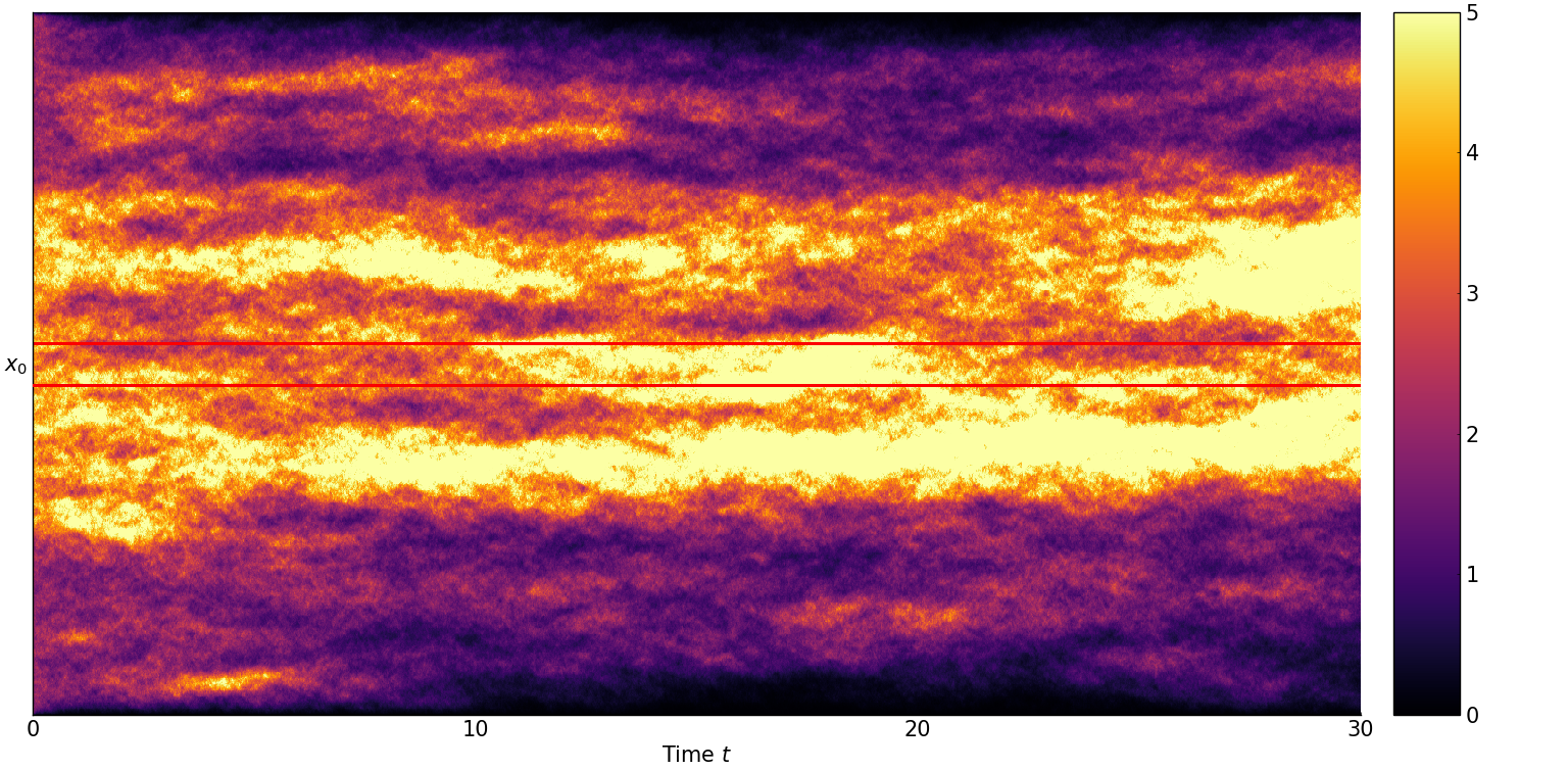 Figure 1
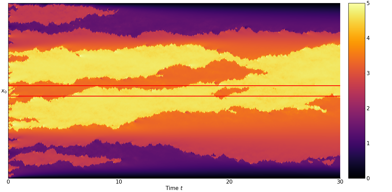 Figure 2
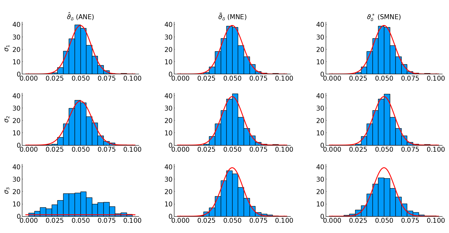 Figure 3
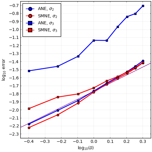 Figure 4
| Mean (SD) | ANE | MNE | SMNE |
|---|---|---|---|
| 0.050183 (0.0104) | 0.050057 (0.0104) | 0.050059 (0.0104) | |
| 0.050632 (0.0111) | 0.050163 (0.0104) | 0.050163 (0.0104) | |
| 0.052085 (0.0522) | 0.050115 (0.0115) | 0.050232 (0.0135) |
Peer Reviews
No public reviews on file for this paper yet. If you reviewed it on a platform where reviews are public (OpenReview, ICLR, NeurIPS, ICML), you can paste yours below so the community can read it here.
Videos
No videos yet. Explain this paper in a talk, walkthrough, or lecture? Add one.
Taxonomy
TopicsStochastic processes and financial applications · Financial Risk and Volatility Modeling · Statistical Methods and Inference
Parameter estimation for the stochastic heat equation with multiplicative noise from local measurements
Josef Janák Markus Reiß Karlsruher Institut für Technologie, Institut für Stochastik, Kaiserstraße 12, 76131 Karlsruhe, Germany. Email: [email protected]ät zu Berlin, Institut für Mathematik, Unter den Linden 6, 10099 Berlin, Germany. Email: [email protected].
Abstract
For the stochastic heat equation with multiplicative noise we consider the problem of estimating the diffusivity parameter in front of the Laplace operator. Based on local observations in space, we first study an estimator, derived in [3] for additive noise. A stable central limit theorem shows that this estimator is consistent and asymptotically mixed normal. By taking into account the quadratic variation, we propose two new estimators. Their limiting distributions exhibit a smaller (conditional) variance and the last estimator also works for vanishing noise levels. The proofs are based on local approximation results to overcome the intricate nonlinearities and on a stable central limit theorem for stochastic integrals with respect to cylindrical Brownian motion. Simulation results illustrate the theoretical findings.
Keywords: Local measurements, stochastic partial differential equation, multiplicative noise, drift estimation, augmented MLE, martingale representation theorem, stable limit theorem.
2020 MSC: Primary 60H15, 60F05; secondary 62G05, 35J15.
1 Introduction
We consider estimation of the diffusivity parameter in the stochastic heat equation with multiplicative noise
[TABLE]
Here, is a cylindrical Brownian motion with values in , is also referred to as space-time white noise. The function generates a multiplicative noise, see Section 2 below for precise assumptions. Multiplicative noise appears naturally in stochastic partial differential equations (SPDEs) as a scaling limit or to ensure positivity of the solution, see e.g. the examples given in [16], [17] or [4].
Diffusivity estimation has emerged as a benchmark inference problem for SPDEs. The spectral estimation approach, initiated by [10], has been shown to give reliable estimation results even for more general semi-linear equations like the stochastic Navier-Stokes equation [7], yet always assuming additive noise. In [8] a specific case of multiplicative noise has been treated which leads to geometric Brownian motions in the spectral decomposition of the Laplacian. In [5] also Bayesian estimators have been developed and analysed in this setting.
Similarly, discrete observations of the solution in time and space give rise to realised -variation estimators for quite general classes of SPDEs. Most notably, in [17] a precise convergence analysis of -variation of in space with and in time with is given, which leads to a consistent diffusivity estimator in the multiplicative noise case, while convergence rates or asymptotic normality are not considered. Estimation of the multiplicative noise function from discrete observations is treated in [6] with intriguing phenomena arising in central limit theorems for -variations.
Recently, methods for local observations in space have provided a new methodology for linear and semi-linear SPDEs with additive noise [3, 2]. This has enabled the estimation of diffusivity in a stochastic cell motility model from experimental data [1]. The underlying SPDE with additive noise describes chemical concentrations, for which, however, a multiplicative noise structure might be more natural as well as more in line with the empirical data than additive noise.
Starting point of our work is the question whether the additive noise estimator (ANE) derived in [3] for local observations of a stochastic heat equation with additive noise is robust against a multiplicative noise misspecification the same way, as it is against nonlinear reaction terms [2]. Technically, we cannot use a splitting technique to separate the nonlinear from the linear part and we must derive new tools to analyse the estimation error. This is achieved by a stepwise disentanglement and localisation of the statistics, carried out in Proposition 5.7 below. The result is that the estimator has the same rate as for additive noise, but it is asymptotically mixed normal under stable convergence with a suboptimal conditional variance for varying .
Therefore we improve the ANE by taking into account the varying quadratic variation of the martingale term in the ANE. The multiplicative noise estimator (MNE) obtained this way satisfies a central limit theorem with smaller variance provided the multiplicative noise is bounded away from zero. Since in many cases it is natural that vanishes at some boundary values, we improve the MNE to the stabilised multiplicative noise estimator (SMNE), satisfying a stable central limit theorem with small conditional variance even when vanishes sometimes.
The exact setting is introduced in Section 2. The construction of the estimators, the main asymptotic results and an application to confidence intervals are presented in Section 3. In Section 4 we discuss the implementation of the estimators and their behaviour for three fundamentally different noise specifications. The detailed proofs are delegated to Section 5. The stable convergence results require a martingale representation theorem in terms of cylindrical Brownian motion and rely on asymptotic orthogonality of martingales by spatial localisation, which might be of independent interest. This material is therefore gathered in Section 6.
2 The model
2.1 Notation
We write , and . By we mean that there exists some constant such that for all values under consideration. Here, we work with or with the convergence . Convergence in probability and convergence in distribution are denoted by and , respectively. The symbol denotes stable convergence, see e.g. [12], Chapter VIII., Section 5. We say that holds on an event if . for random variables means that is tight, that is, as . The notation stands for as .
Let be an open bounded interval in and consider the space equipped with the usual -norm and the scalar product . denotes the -Sobolev space of order on and the space of all with for . The Laplace operator is given by for , even though we consider only the one-dimensional case.
2.2 The stochastic heat equation
Let be a stochastic basis equipped with the cylindrical Brownian motion taking values in . The filtration is assumed to be generated by the cylindrical Brownian motion and augmented by –null sets. We study the stochastic heat equation (1.1) with multiplicative noise. The initial value is supposed to be deterministic and continuous on . We require throughout the following two assumptions.
Assumption (S)****.
The function is continuous and
[TABLE]
The stochastic term is therefore understood as with the multiplicative Nemytskii operators , defined by
[TABLE]
noting that holds for bounded .
Assumption (X)****.
The stochastic partial differential equation (1.1) admits a weak solution taking values in , which is continuous in both (time and space) variables, i.e., –a.s., and satisfies for any and
[TABLE]
Sufficient conditions for Assumption (X) will be discussed in Example 3.7 below. Since a weak solution is also a mild solution (see e.g. Theorem 6.5 in [9]), there is an additional representation of the solution to equation (1.1). Let be the strongly continuous semigroup on generated by . The solution satisfies the variation-of-constants formula
[TABLE]
2.3 The observation scheme
As motivated in [3, 1], we observe the solution process only locally in space around some point , which remains fixed like the observation time . More precisely, the observations are given by a spatial convolution of the solution process with a kernel , localising at as the resolution tends to zero. This kernel might for instance model the point spread function in microscopy.
For and introduce the scalings
[TABLE]
Let be a function of compact support in . The compact support ensures that is localising around as and that . The scaling with simplifies calculations due to , while the basic estimators are invariant with respect to kernel scaling.
Local measurements of (1.1) at the point with resolution level are described by the real-valued processes and given by
[TABLE]
The process satisfies and by partial integration
[TABLE]
3 Estimation methods and main results
3.1 The additive noise estimator
We study first the augmented maximum likelihood estimator from [3], derived for the stochastic heat equation with additive space-time white noise.
Definition 3.1**.**
The additive noise estimator (ANE) of the parameter is defined as
[TABLE]
According to (2.5), the numerator equals
[TABLE]
and the fundamental error decomposition is given by
[TABLE]
where
[TABLE]
The term is incorporated because it gives the quadratic variation of the martingale in time. It turns out that converges in probability to the limit as , while converges to , see Proposition 5.10 below. Since the quadratic variation does not become asymptotically deterministic, we cannot rely on a standard martingale central limit theorem to prove asymptotic normality of . Therefore we employ the concept of stable convergence, which allows to formulate mixed normal limits and to derive data-driven confidence intervals, see e.g. [12] for a general introduction. In Section 6 we prove a general martingale representation theorem and a stable limit theorem for martingales with respect to cylindrical Brownian motion filtrations. As a consequence, we obtain the following result, when specialising Corollary 6.3 to our setting involving the kernels :
Proposition 3.2**.**
Let for be -valued processes, progressively measurable with respect to the cylindrical Brownian filtration and satisfying . If
- (C1)
* as for some progressively measurable real-valued process with ,*
- (C2’)
the support inclusion holds Lebesgue-almost everywhere in for all ,
then a stable limit theorem for the stochastic integrals holds as :
[TABLE]
with an independent scalar Brownian motion (on an extension of the original filtered probability space).
The main point of this result is that the limiting Brownian motion becomes independent because the support of shrinks asymptotically to the point . Here we shall apply the proposition with . Our first main result is that the additive noise estimator satisfies a stable central limit theorem with rate .
Theorem 3.3**.**
Grant Assumptions (S) and (X). Then the ANE satisfies on the event
[TABLE]
as , where is independent of .
Proof.
The detailed proof is deferred to Section 5.4. ∎
This result establishes a very desirable robustness property of the ANE : Even though it was designed for estimation in the stochastic heat equation with additive noise, the ANE still converges with the same rate to the true parameter under multiplicative noise.
3.2 The multiplicative noise estimator
We aim at improving the ANE by adjusting the estimator in such a way that the denominator contains already the quadratic variation of the martingale part in the numerator. To that end, we need to incorporate the term that is not observed directly, but is still attainable from the data. The quadratic variation of the observed semi-martingale equals
[TABLE]
So we have access to by differentiation of the realized quadratic variation. For discrete time data, sampled at high-frequency, standard spot volatility estimators can be used to access this term, see Section 4 below. This way we obtain a second estimator, taking into account the multiplicative noise in the stochastic heat equation.
Definition 3.4**.**
The multiplicative noise estimator (MNE) of the parameter is defined as
[TABLE]
Let us remark that the MNE can also be derived like the ANE in [3], maximising a corresponding pseudo-likelihood in the multiplicative noise case. Since this is done under the correct model specification, we expect better estimation properties.
Using the representation of from (2.5), we obtain
[TABLE]
Since appears in the denominators, we require a lower bound on in the following theorem.
Theorem 3.5**.**
Grant Assumptions (S), (X) and assume . Then as
[TABLE]
Proof.
The proof is deferred to Section 5.4. ∎
3.3 The stabilised multiplicative noise estimator
The lower bound on required for the MNE can be restrictive. For instance, when the random field shall not take negative values, models usually require that . To cover this case as well, we stabilise the denominators by adding a number which tends to zero slowly as .
Definition 3.6**.**
Let be a real function satisfying for any
[TABLE]
as . Then the stabilised multiplicative noise estimator (SMNE) of the parameter is defined as
[TABLE]
Condition (3.8) says that tends to zero more slowly than any polynomial. It is satisfied for . To analyse the asymptotic properties of the SMNE , we need to strengthen Assumptions (S) and (X) slightly.
Assumption (S’)****.
Assumption (S) is satisfied and is –Hölder continuous, i.e., for some there exists a constant such that
[TABLE]
Assumption (X’)****.
Assumption (X) is satisfied and moreover the solution is in quadratic mean –Hölder continuous in the space variable and –Hölder continuous in the time variable, i.e., for some there is a constant with
[TABLE]
Example 3.7**.**
If is Lipschitz continuous, then standard contraction arguments for the stochastic convolution and the regularity of the Green function for the heat equation yield Assumption (X’) with and , provided the initial condition is –Hölder continuous. Assumption (X) holds already for a continuous initial condition and Lipschitz continuous . In fact, standard proofs for pathwise Hölder regularity go via the Kolmogorov-Chentsov theorem and thus establish (3.10), compare Theorem 2.1 in [17] or Corollary 3.4 in [19] for a slightly more involved case on an unbounded domain.
The intriguing questions of weak existence, regularity and pathwise uniqueness for the stochastic heat equation with -Hölder continuous multiplicative noise have so far only found partial answers. We refer to Theorem 1.3 in [16], which yields our Assumption (X) in case in case of an unbounded domain. For their continuity result the authors assert that the results in [18], formulated for coloured noise in space, work analogously for the space-time white noise case. Equations (10) and (19) in [18] then establish Hölder regularity of in the sense of Assumption (X’).
We turn to the analysis of the stabilised multiplicative noise estimator. The error decomposition for the SMNE follows from (3.9) and (2.5):
[TABLE]
with
[TABLE]
The term is the quadratic variation of the martingale part . The limits of and for involve an (in general random) time length during which does not vanish, see Proposition 5.10 below. So, we use again the stable limit theorem of Proposition 3.2 and derive a central limit theorem for the SMNE with rate , without assuming a lower bound on .
Theorem 3.8**.**
Grant Assumptions (S’) and (X’) with (3.8). Introduce
[TABLE]
Then as on the event
[TABLE]
where is independent of .
Proof.
The proof is deferred to Section 5.4. ∎
Remark 3.9**.**
From the series of inequalities
[TABLE]
we infer that the (conditional) asymptotic variance of the SMNE lies between those of the ANE and the MNE. Remember, however, that the asymptotics for the MNE were derived under the condition , implying . The extreme case leads to the deterministic heat equation, which for the initial condition remains zero all the time and does not allow for inference on . This type of degeneracy is excluded for the SMNE by the condition .
3.4 Data-driven confidence intervals
The asymptotic (mixed) normality of the three estimators allows us to prescribe asymptotic confidence intervals for the parameter . The asymptotic conditional variances depend on quantities unknown to the statistician. Yet, in all three error decompositions (3.2), (3.6) and (3.11) it is shown in the proofs that the martingale term divided by the square root of its quadratic variation is asymptotically standard Gaussian. Dividing each error decomposition by the respective second factor on the right-hand side directly gives an asymptotic confidence statement.
Corollary 3.10**.**
Let . Based on the three estimators , and the confidence intervals for
[TABLE]
with the standard Gaussian -quantile have each asymptotic coverage as under the assumptions of Theorems 3.3, 3.5 and 3.8, respectively.
Note that the confidence intervals only rely on the observation processes , and the quadratic variation of the latter. Even the kernel and the resolution level need not be known. In the next section we shall see how the estimation methods can be implemented when only data is available that is discretely sampled in time.
4 Implementation and simulation results
We illustrate the main results in a setting similar to the experimental setup in [1], where the diffusivity parameter was estimated in a concrete stochastic model for cell repolarisation.
Consider the stochastic heat equation (1.1) with for , , . The initial condition is a smooth approximation of the function . We present the results for three different functions :
[TABLE]
We have chosen to have Hölder regularity 0.8 in line with Example 3.7 and not to vanish completely at zero so that all three estimators are applicable. generates strong noise level fluctuations so that the quality of the estimators should differ significantly.
An approximate solution is computed on a regular time-space grid with and by the Euler-Maruyama scheme. For the drift part, we use the finite difference approximation of that is applied implicitly, while in the stochastic term is applied to the current state of the solution explicitly, compare Algorithm 10.8 in [15]. The mesh sizes fulfill , ensuring the Courant-Friedrichs-Lewy (CFL) condition for stable simulations [15]. Heat maps for typical realisations with multiplicative noise and are displayed in Figure 1. Under we see that fluctuations are larger for higher temperature levels, while at the boundary it cools down to zero almost deterministically. Under excitations by strong noise at the interface values 2 and 4 are counteracted by the diffusion, which leads to almost noiseless inner regions with strong fluctuations of the interfaces in time. The spatial gradient at the interfaces is very large, which is no numerical artefact, but due to expulsion by noise.
As in [1] we employ the smooth compactly supported kernel
[TABLE]
and we localise around the central point with . Based on these local measurements, the estimators (ANE), (MNE) and (SMNE) are computed.
The term is accessed by the following procedure. In view of (3.4), presents the spot volatility of at time , which we estimate by
[TABLE]
i.e., by taking the average disintegrated realised quadratic variation over the past values ( time units). The averaging acts as a smoothing, which is a standard approach for spot volatility estimation [11].
Finally, we choose the stabilising value such that it satisfies condition (3.8) and lies within the range of typical values of . The possible issue could be that if the term is much smaller than , the SMNE would practically become the MNE. On the other hand, if the term dominated , then the SMNE would practically coincide with the ANE. So, in practice we recommend to estimate the spot volatility first and then to adjust accordingly.
Figure 2 displays simulation results for the estimators of the parameter obtained after Monte Carlo runs for each of the functions , and . The red lines in the histograms indicate the asymptotic distribution, obtained as a mixture of Gaussian densities that (individually, for each run) follow the theoretical results established in Theorems 3.3, 3.5 and 3.8. Monte Carlo mean and standard deviation for every case are stated in Table 1.
In the additive noise case all three estimators perform similarly well. In this case we have equalities in (3.13) and the resulting asymptotic distributions coincide. In the “Hölder” multiplicative noise case , the estimator ANE performs slightly worse than the two alternatives. Since , we have and the estimators MNE and SMNE deliver similar results.
For the histogram of the ANE in Figure 2(bottom, left) is much more spread out, but has not yet entered the asymptotic regime with a very flat asymptotic density. There are, however, quite a few outliers (12.6 %) outside the interval , which are not shown and which are caught pretty well by the tails of the asymptotic density. Note also that the corresponding empirical standard deviation in Table 1 is very high with about half the length of the interval . The estimators MNE and SMNE give a significant improvement here with an error distribution that is almost unchanged with respect to the cases and . It is worth noting that the assumption from Theorem 3.5 for the MNE is violated by and we also had , but with a minor difference only. In the discrete numerical setting we use the threshold to determine whether is zero or not.
Further unreported simulations show that the performance of the estimators is not influenced by the location of the central observation point , unless is located very close to the boundary. In fact, if several local measurements (localised around points ) are available, it is possible to combine local estimators, see [1], where such an approach is explained and used. Also, simulation results for varying confirm the convergence rate as . Note, however, that the spatial discretisation for reliable simulations must always be much finer than . In our setup with and , the localised kernel was evaluated discretely on grid points.
In conclusion, the two newly proposed estimators MNE and SMNE performed as well as the ANE or even better than the ANE and their asymptotic distribution matches the results obtained in Section 3. The ANE provides good estimation accuracy also under multiplicative noise, but its accuracy suffers under strongly varying .
5 Proofs
5.1 Fundamental asymptotics
We need some properties of the rescaled operators and semigroups. Let be the strongly continuous semigroup generated by with Dirichlet boundary conditions on and note that both semigroups and , are self-adjoint. We cite Lemma 3.1 from [3]:
Lemma 5.1**.**
For the following holds:
- (i)
If , then .
- (ii)
If , then , .
The deterministic flow of the initial condition will become negligible due to the next result.
Lemma 5.2**.**
For an initial condition we have
[TABLE]
Proof.
Lemma A.7(ii) in [3] shows for , , that
[TABLE]
Because of we may choose and obtain the result. ∎
Lemma 5.3**.**
Grant Assumptions (S) and (X). For any ,
[TABLE]
holds as . The limit holds true for any , i.e., surely.
Proof.
For any , we have by the continuity of and , provided by Assumptions (S) and (X),
[TABLE]
Here dominated convergence is applied with integrable majorant . ∎
We will need an inequality for the rescaled semigroup . It encapsulates essentially the hypercontractivity of the heat semigroup.
Lemma 5.4**.**
For , and we have
[TABLE]
Proof.
For we apply Lemma A.6(ii) from [3] with , and . The constant involved only depends on and , which are fixed here.
For we combine Proposition 3.5(i) in [3] and the second inequality from Lemma A.2(iii) in [3] such that
[TABLE]
with , using that has compact support and is fixed throughout.
For we use the Hölder inequality with weight function and to obtain
[TABLE]
where we used the first two parts of the proof. ∎
We need a uniform bound on the second and fourth centered moment of in the sequel.
Lemma 5.5**.**
For we have
[TABLE]
in particular we have uniformly over .
Proof.
[TABLE]
The Burkholder-Davis-Gundy inequality yields with a constant
[TABLE]
Setting and , we obtain
[TABLE]
Note that inequality (5.2) holds uniformly over and gives the result. The second part follows via Jensen’s inequality. ∎
5.2 Approximation of quadratic variations and related terms
We are ready to study the asymptotic behaviour of the terms , , , and . We will analyse them simultaneously, using a generalisation .
First, let be a continuous (and possibly non-linear) functional of the state, satisfying one of the following:
- (F1)
There exists such that for any ,
[TABLE]
- (F2)
There exists such that for any ,
[TABLE]
where is satisfying (3.8).
Lemma 5.6**.**
- (i)
Functionals satisfy condition (F1), provided in the last case.
- (ii)
Functionals satisfy condition (F2).
Proof.
(i). For the statement is trivial.
For we have a uniform upper bound . Moreover, for any and we have
[TABLE]
where we used together with the upper bound in the first inequality and then we followed up with the reverse triangle inequality.
For , there is a uniform upper bound . Moreover, for any and we have
[TABLE]
Therefore the proof is finished as in the previous case.
(ii). For the upper bound is smaller than . To prove the second part, we use , the upper bound and the reverse triangle inequality to obtain
[TABLE]
For , the upper bound applies. Moreover, algebraic calculations and the technique above yield
[TABLE]
Therefore, the proof is finished as in the previous case. ∎
Introduce
[TABLE]
In the following proposition we present different expressions that are equal to up to terms that are of lower order than . This is the major ingredient for the proofs of the main results, noting that the techniques developed in [3] cannot be used here due to the multiplicative noise structure.
Proposition 5.7**.**
Grant Assumptions (S), (X) with satisfying condition (F1) or grant Assumptions (S’), (X’) with (3.8) and satisfying condition (F2). Then from (5.3) equals up to additive terms of order for :
- (i)
**
- (ii)
**
- (iii)
,
- (iv)
,
- (v)
,
- (vi)
.
- (vii)
.
Remark 5.8**.**
The overall idea is to achieve the representation via slight consecutive alterations. In point (i) we shorten the outer integral to the interval , in (ii), we present a slight time shift of the solution in the functional, i.e., . In point (iii) the function is fixed in the space-point , in (iv) the stochastic integral is shortened, in (v) the function is fixed at the time-point . In (vi) the expectation of the squared stochastic integral is implemented via conditional independence. Finally, in (vii) the expectation is approximated and the integral extended again.
Proof.
We present the proof with Assumptions (S’) and (X’) and satisfying condition (F2) with (3.8) in mind. The other case is analogous and much simpler, mostly because it does not use the function at all. The proof of (ii) is shown for both cases. The order for is used frequently as the first step of the proof.
(i). Compute
[TABLE]
using Lemma 5.5. Therefore, the remainder term is of order due to by (3.8).
(ii). By the Cauchy-Schwarz inequality, we have
[TABLE]
Lemma 5.5 gives so that the second factor is of order . Hence, it suffices to establish .
When we consider Assumptions (S’), (X’) and satisfying condition (F2), we obtain
[TABLE]
by the Hölder continuity of and and by . This upper bound converges to zero by (3.8).
When we consider Assumptions (S), (X) and satisfying condition (F1), we have
[TABLE]
The integrand in (5.6) converges to zero by the continuity of and (i.e., Assumptions (X) and (S)). The integrable majorant serves for the –integral in (5.6) as well as for the –integral in (5.5). The proof that the second factor converges almost surely to zero is accomplished by the dominated convergence theorem.
(iii). By the upper bound on , we have
[TABLE]
Denoting
[TABLE]
using and the Cauchy-Schwarz inequality, we may follow up (5.7) with
[TABLE]
We start with the first factor after . Itô’s isometry yields
[TABLE]
and this is of order , compare (5.2). The second factor is given by
[TABLE]
Using Assumptions (S’) and (X’), we have
[TABLE]
and consequently for the integrand in (5.10)
[TABLE]
Without loss of generality assume and (otherwise decrease or slightly). Using Lemma 5.4, we obtain from (5.11)
[TABLE]
Since the bound applies uniformly to all , we deduce from (5.10)
[TABLE]
in view of (3.8), which remained to be proved.
(iv). We obtain, using the Cauchy-Schwarz inequality,
[TABLE]
In the analysis of , we use Itô’s isometry, the scaling properties from Lemma 5.1 and Lemma 5.4 with . We obtain
[TABLE]
due to (3.8). Given the result for , term is also of order because the squared second factor is of order :
[TABLE]
using Itô isometry and arguing as in (5.2).
(v). Denoting
[TABLE]
we compute
[TABLE]
Itô’s isometry yields
[TABLE]
Hence, follows from the boundedness of and the argument in (5.2).
For the term with we have from Assumptions (S’) and (X’) that uniformly over and . The same argument thus gives here . Insertion into (5.13) and noting condition (3.8) yields the overall rate .
(vi). Introduce for
[TABLE]
and compute
[TABLE]
We analyse the integral on two sets: (a) and (b) .
(a) . We condition on and obtain
[TABLE]
using that is independent of with and that the other factors are -measurable.
(b) . In this case, we use the upper bounds for and and bound (5.14) (up to a positive constant) by
[TABLE]
where the last step involves the Cauchy-Schwarz inequality. The analogous calculations to (5.2) yield
[TABLE]
uniformly over . We conclude , implying due to (3.8).
(vii). By translating the integrand in and by Itô’s isometry we have
[TABLE]
By the uniforms bounds on and the last term is of order .
Next, we compute by the scaling properties in Lemma 5.1 and by partial integration
[TABLE]
Now, bounding the scalar product by the Cauchy-Schwarz inequality and Lemma 5.4 with , we see that it is of order . Using the upper bounds for and again, we thus obtain
[TABLE]
by (3.8). ∎
5.3 Asymptotics of quadratic variations and related terms
We shall include the initial condition and consider the terms
[TABLE]
where is not centered. Having achieved the representation , we are now ready to determine the limit of as .
Corollary 5.9**.**
Grant Assumptions (S), (X) with satisfying condition (F1) or grant Assumptions (S’), (X’) with (3.8) and satisfying condition (F2). Suppose as
[TABLE]
for some random variable . Then from (5.16) satisfies for
[TABLE]
Proof.
The corresponding convergence for the centered version follows directly from the representation (vii) in Proposition 5.7.
For note that
[TABLE]
We apply the upper bound to from condition (F1) (respectively (F2)) to the first term and obtain its convergence to zero by Lemma 5.2 using due to (3.8) in the second case. The second term converges to zero in probability using the Cauchy-Schwarz inequality and from above. This gives the result for . ∎
Proposition 5.10**.**
The following holds as :
- (i)
under Assumptions (S) and (X):
[TABLE]
- (ii)
under Assumptions (S) and (X):
[TABLE]
- (iii)
under Assumptions (S) and (X) and assuming :
[TABLE]
- (iv)
under Assumptions (S’) and (X’) with (3.8):
[TABLE]
- (v)
under Assumptions (S’) and (X’) with (3.8):
[TABLE]
Proof.
We apply Proposition 5.9 to the functionals proposed in Lemma 5.6.
(i). We use so that and the result follows.
(ii). We use . Since by Lemma 5.3, the limit follows by dominated convergence because is an integrable majorant.
(iii). We use . Since , we obtain the limit . The integrable majorant for the –integral over can be taken as (up to a multiplicative constant).
(iv). We use . Since we have only an upper bound to in this case, obtaining an integrable majorant to is not so straightforward. We use , the upper bound and Assumptions (S’) and (X’) to obtain
[TABLE]
This gives the uniform majorant in and
[TABLE]
for sufficiently small due to (3.8). Next, we determine the pointwise limit of the -distance. In view of (5.18) and due to (3.8) it suffices to note for all
[TABLE]
We conclude that the integral converges in and thus in probability to
[TABLE]
(v). We use . An integrable majorant in is given by and the limit is determined as in the previous case. ∎
5.4 Proof of the main theorems
Proof of Theorem 3.3.
Consider the error decomposition (3.2). The asymptotic properties of and are established in Proposition 5.10(i),(ii), therefore the second factor converges in probability to the random variable
[TABLE]
For the first factor, let and check the two conditions of Proposition 3.2. Since
[TABLE]
by Proposition 5.10(ii), condition (C1) is satisfied with . The support condition (C2’) follows directly from the definition of as a multiple of . Proposition 3.2 thus shows as with an independent scalar Brownian motion . On the event we infer where is independent of the –algebra . We conclude by applying Slutsky’s lemma. ∎
Proof of Theorem 3.5.
The decomposition of the error follows from (3.6):
[TABLE]
A standard continuous martingale central limit theorem (e.g., [14], Theorem 1.19) provides the convergence of the first factor to in distribution.
Proposition 5.10(iii) yields the convergence
[TABLE]
The result follows by applying Slutsky’s lemma. ∎
Proof of Theorem 3.8.
Consider the error decomposition (3.11). The asymptotic properties of and are established in Proposition 5.10(iv),(v). Therefore the second factor converges in probability to the random variable
[TABLE]
For the first factor, let and check the two conditions of Proposition 3.2. Since
[TABLE]
by Proposition 5.10(v), condition (C1) is satisfied with . The support condition (C2’) follows again directly by definition of .
Proposition 3.2 thus yields with an independent scalar Brownian motion . Hence, holds on with independent of the –algebra . The proof is concluded by applying Slutsky’s lemma. ∎
6 A stable limit theorem for cylindrical Brownian martingales
Let be a separable Hilbert space and a complete orthonormal system in . Let be a sequence of independent real-valued standard Brownian motions. Then is an -valued cylindrical Brownian motion (e.g., Proposition 4.11 in [9]). Consider the filtered probability space , on which are defined and where the Brownian filtration is the filtration generated by and augmented by –null sets.
We start with a Hilbert space-valued Brownian martingale representation theorem, which follows by approximation from the finite-dimensional version, but does not seem readily available in the literature.
Proposition 6.1**.**
Let be a square-integrable real-valued martingale with respect to and with càdlàg paths, . Then there exist progressively measurable processes satisfying for all and –a.s. (with -convergence)
[TABLE]
where .
Proof.
Define the subfiltrations generated by and consider
[TABLE]
By the tower property for , we have
[TABLE]
and another application of the tower property yields
[TABLE]
We conclude that forms an -martingale with respect to the -dimensional Brownian filtration . By standard martingale theory (e.g., Theorem 1.3.13 in [13]) we may choose a càdlàg version of , which we shall do henceforth.
Theorem 3.4.15 in [13] therefore shows that there are satisfying for all and –a.s.
[TABLE]
The uniqueness result of that theorem also shows that for each the , , can be chosen to not depend on because by independence of from , , we have
[TABLE]
Since is generated by , the -martingale convergence theorem gives in -convergence for every . Hence, also converges in for . By Itô’s isometry this shows that the -norms converge: . The limit is then well defined as an element of . Moreover, it equals the limit of whence
[TABLE]
holds –a.s. for each fixed . Using the càdlàg path versions on each side, this entails equality for all with probability one. ∎
Theorem 6.2**.**
Let for be progressively measurable -valued processes on with and all (or ). Assume for all :
- (C1)
* as for some progressively measurable real-valued process with ,*
- (C2)
* as for all progressively measurable -valued processes .*
Then the following stable limit theorem for stochastic integrals holds:
[TABLE]
with an independent scalar Brownian motion (on an extension of the original filtered probability space).
Proof.
Since is a continuous martingale with quadratic variation , we can apply Theorem IX.7.3(b) in [12] with the trivial processes , (in that Theorem), so that it remains to check for all :
- (i)
, 2. (ii)
for all bounded càdlàg-martingales on with .
Condition (i) is satisfied by assumption (C1). For condition (ii) we use the Brownian martingale representation from Proposition 6.1 to represent with progressively measurable coordinates and for all . Then holds and condition (ii) follows from Assumption (C2). ∎
Corollary 6.3**.**
Theorem 6.2 holds for if condition (C2) is replaced by the following support condition:
- (C2’)
There exist deterministic Borel sets with Lebesgue-almost everywhere for all and as , where denotes Lebesgue measure on .
Proof.
Set for in condition (C2) of Theorem 6.2. Then by and dominated convergence, holds in for each . Clearly, for each the support property gives
[TABLE]
By the triangle and the Cauchy-Schwarz inequality and using condition (C1), we obtain
[TABLE]
with convergence in probability. ∎
Acknowledgment
We are grateful to Randolf Altmeyer for very helpful discussions, in particular bringing up the ideas for Proposition 5.7. Insightful comments and questions by Gregor Pasemann, Eric Ziebell and Pavel Kříž have lead to several improvements. This research has been funded by Deutsche Forschungsgemeinschaft (DFG) - SFB1294/1 - 318763901.
The reference list from the paper itself. Each links out to its DOI / PubMed record.
- 1[1] R. Altmeyer, T. Bretschneider, J. Janák, M. Reiß (2022) Parameter estimation in an SPDE model for cell repolarisation, SIAM/ASA J. Uncert. Quantif. 10 , 179–199.
- 2[2] R. Altmeyer, I. Cialenco, G. Pasemann (2020) Parameter estimation for semilinear SPD Es from local measurements, Preprint , ar Xiv:2004.14728.
- 3[3] R. Altmeyer, M. Reiß (2021) Nonparametric estimation for linear SPD Es from local measurements, Ann. Appl. Probab. 31 , 1–38.
- 4[4] J. Blath, M. Hammer, F. Nie (2022) The stochastic Fisher-KPP equation with seed bank and on/off branching coalescing Brownian motion, Stoch. PDE: Anal. Comp. , 1–46.
- 5[5] Z. Cheng, I. Cialenco, R. Gong (2020) Bayesian estimations for diagonalizable bilinear SPD Es, Stoch. Proc. Appl. 130 , 845–877.
- 6[6] C. Chong (2019) High-frequency analysis of parabolic stochastic PD Es with multiplicative noise: Part I, Preprint , ar Xiv:1908.04145.
- 7[7] I. Cialenco, N. Glatt-Holtz (2011) Parameter estimation for the stochastically perturbed Navier-Stokes equations, Stoch. Proc. Appl. 121 , 701–724.
- 8[8] I. Cialenco, S. Lototsky (2009) Parameter estimation in diagonalizable bilinear stochastic parabolic equations, Stat. Infer. Stoch. Proc. 12 , 203–219.