Learning time-scales in two-layers neural networks
Rapha\"el Berthier, Andrea Montanari, Kangjie Zhou

TL;DR
This paper investigates the multi-scale and intermittent learning dynamics of two-layer neural networks in high-dimensional settings, revealing how different phases of training occur on distinct time scales.
Contribution
It provides a new theoretical framework for understanding the separation of time scales and intermittency in neural network training dynamics.
Findings
Identification of multiple learning time scales.
Demonstration of intermittency in gradient flow.
Validation through numerical simulations.
Abstract
Gradient-based learning in multi-layer neural networks displays a number of striking features. In particular, the decrease rate of empirical risk is non-monotone even after averaging over large batches. Long plateaus in which one observes barely any progress alternate with intervals of rapid decrease. These successive phases of learning often take place on very different time scales. Finally, models learnt in an early phase are typically `simpler' or `easier to learn' although in a way that is difficult to formalize. Although theoretical explanations of these phenomena have been put forward, each of them captures at best certain specific regimes. In this paper, we study the gradient flow dynamics of a wide two-layer neural network in high-dimension, when data are distributed according to a single-index model (i.e., the target function depends on a one-dimensional projection of the…
Click any figure to enlarge with its caption.
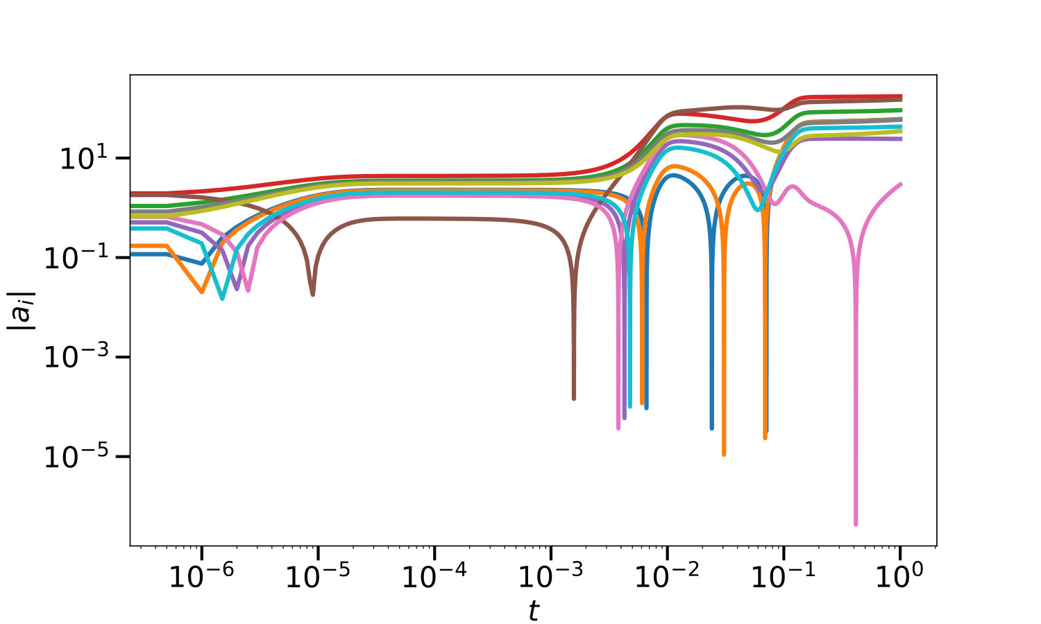 Figure 1
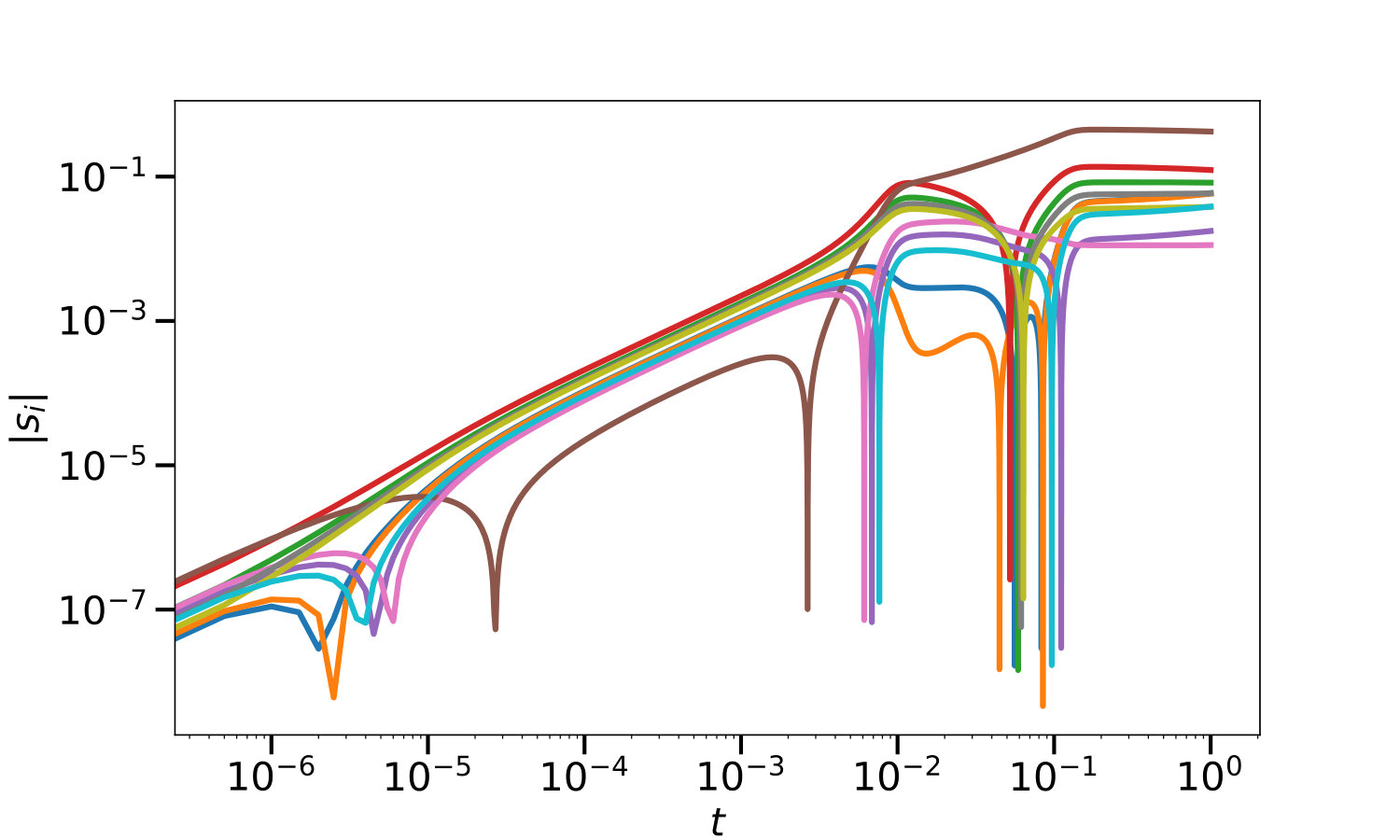 Figure 2
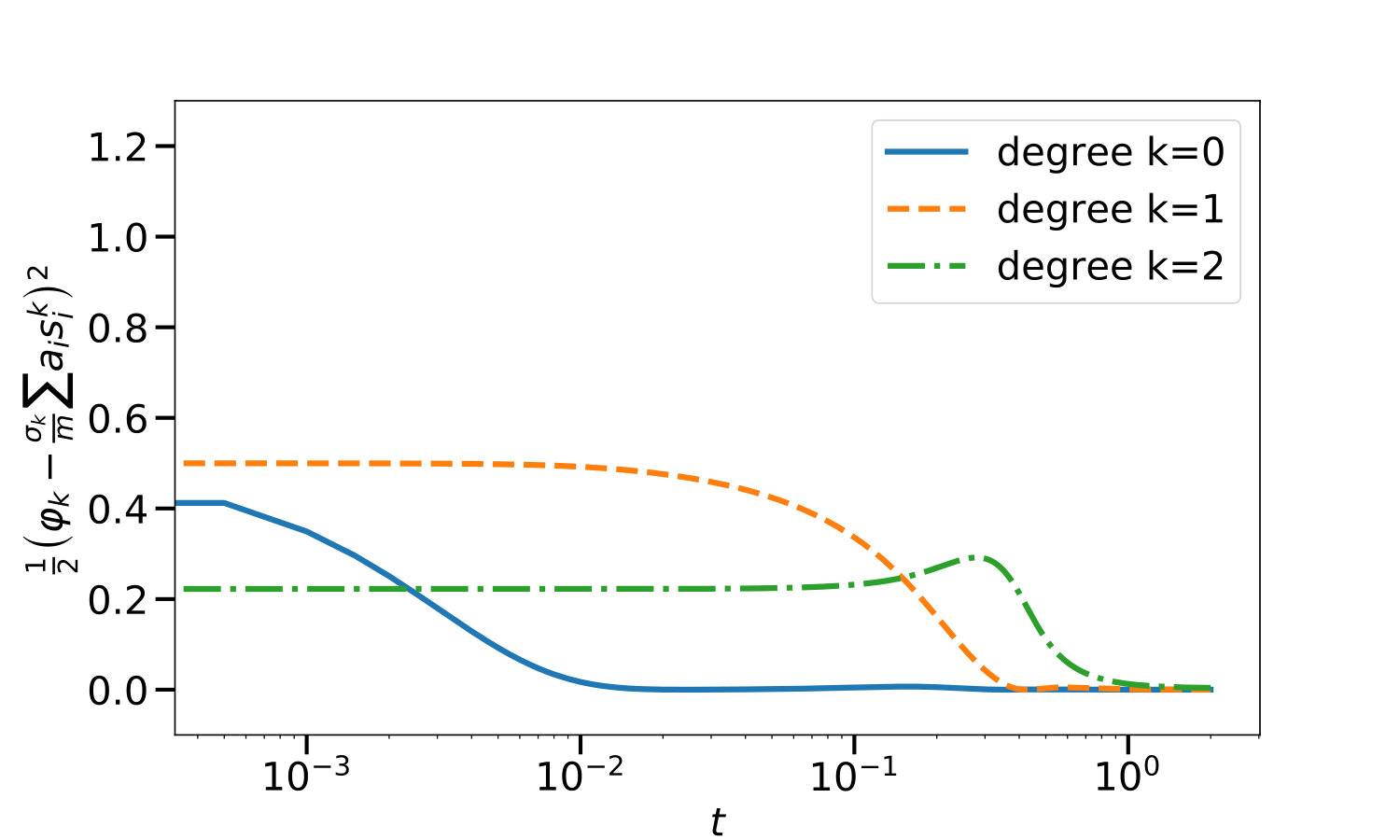 Figure 3
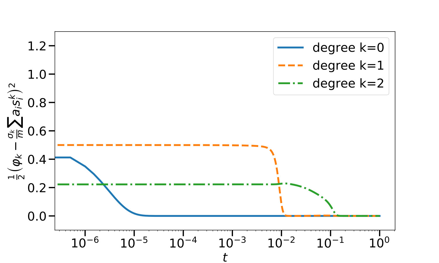 Figure 4
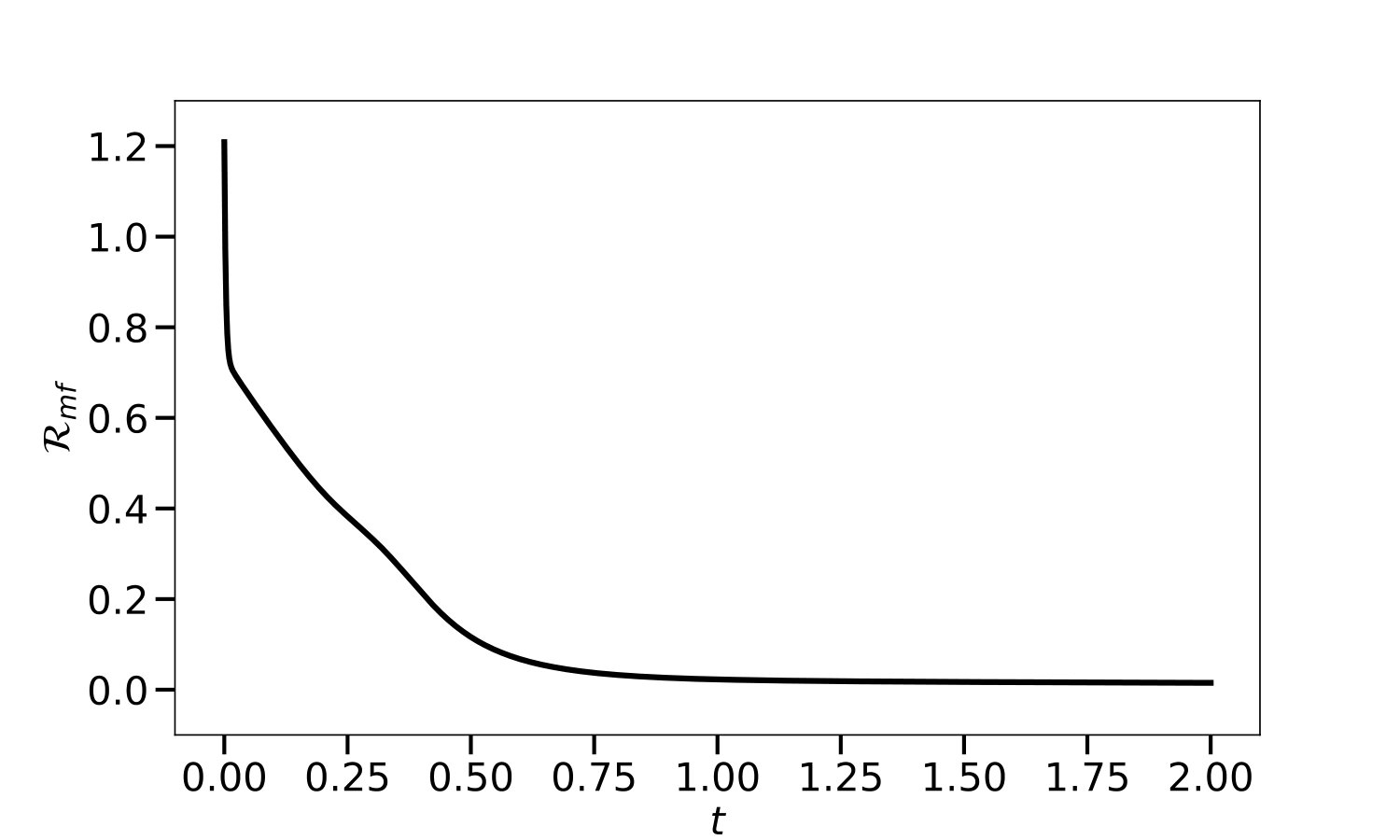 Figure 5
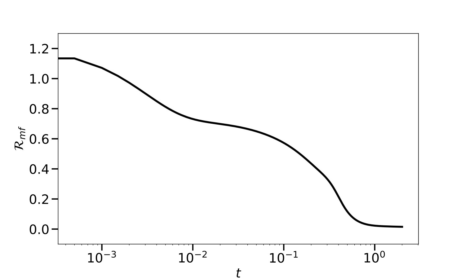 Figure 6
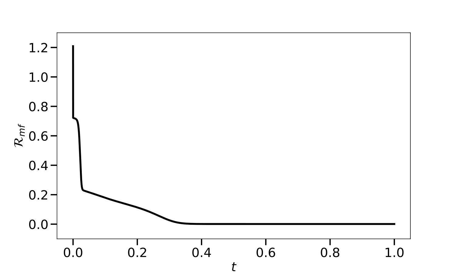 Figure 7
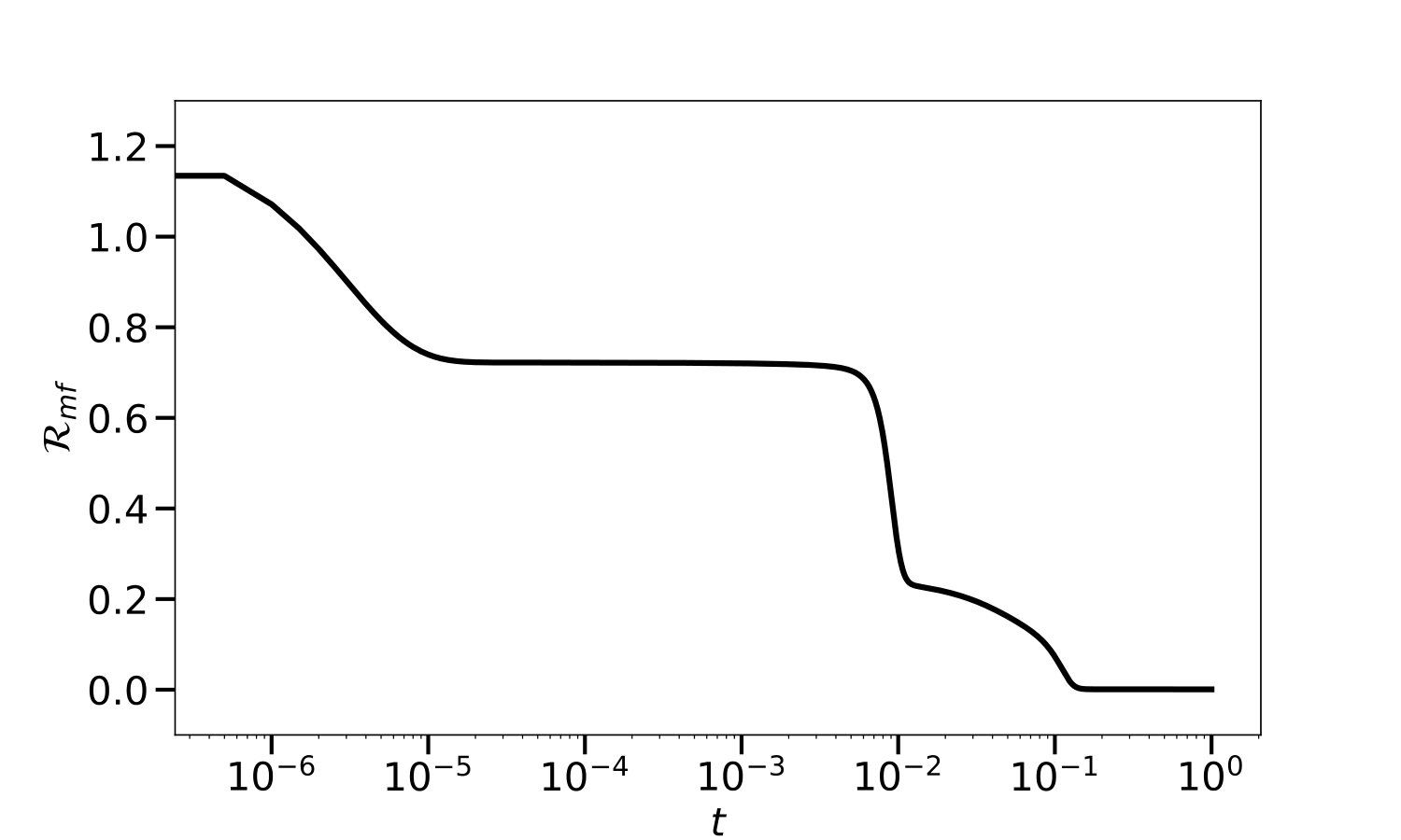 Figure 8
Peer Reviews
No public reviews on file for this paper yet. If you reviewed it on a platform where reviews are public (OpenReview, ICLR, NeurIPS, ICML), you can paste yours below so the community can read it here.
Videos
No videos yet. Explain this paper in a talk, walkthrough, or lecture? Add one.
Taxonomy
TopicsNeural Networks and Applications · Model Reduction and Neural Networks · Stochastic Gradient Optimization Techniques
Learning time-scales in two-layers neural networks
Raphaël Berthier, Andrea Montanari, Kangjie Zhou EPFLDepartment of Electrical Engineering and Department of Statistics, Stanford UniversityDepartment of Statistics, Stanford University
Abstract
Gradient-based learning in multi-layer neural networks displays a number of striking features. In particular, the decrease rate of empirical risk is non-monotone even after averaging over large batches. Long plateaus in which one observes barely any progress alternate with intervals of rapid decrease. These successive phases of learning often take place on very different time scales. Finally, models learnt in an early phase are typically ‘simpler’ or ‘easier to learn’ although in a way that is difficult to formalize.
Although theoretical explanations of these phenomena have been put forward, each of them captures at best certain specific regimes. In this paper, we study the gradient flow dynamics of a wide two-layer neural network in high-dimension, when data are distributed according to a single-index model (i.e., the target function depends on a one-dimensional projection of the covariates). Based on a mixture of new rigorous results, non-rigorous mathematical derivations, and numerical simulations, we propose a scenario for the learning dynamics in this setting. In particular, the proposed evolution exhibits separation of timescales and intermittency. These behaviors arise naturally because the population gradient flow can be recast as a singularly perturbed dynamical system.
Contents
1 Introduction
It is a recurring empirical observation that the training dynamics of neural networks exhibits a whole range of surprising behaviors:
Plateaus. Plotting the training and test error as a function of SGD steps, using either small stepsize or large batches to average out stochasticity, reveals striking patterns. These error curves display long plateaus where barely anything seems to be happening, which are followed by rapid drops (Saad and Solla, 1995; Yoshida and Okada, 2019; Power et al., 2022). 2. 2.
Time-scales separation. The time window for this rapid descent is much shorter than the time spent in the plateaus. Additionally, subsequent phases of learning take increasingly longer times (Ghorbani et al., 2020a; Barak et al., 2022). 3. 3.
Incremental learning. Models learnt in the first phases of learning appear to be simpler than in later phases. Among others, Arpit et al. (2017) demonstrated that easier examples in a dataset are learned earlier; Kalimeris et al. (2019) showed that models learnt in the first phase of training correlate well with linear models; Gissin et al. (2019) showed that, in many simplified models, the dynamics of gradient descent explores the solution space in an incremental order of complexity; Power et al. (2022) demonstrated that, in certain settings, a function that approximates well the target is only learnt past the point of overfitting.
Understanding these phenomena is not a matter of intellectual curiosity. In particular, incremental learning plays a key role in our understanding of generalization in deep learning. Indeed, in this scenario, stopping the learning at a certain time amounts to controlling the complexity of the model learnt. The notion of complexity corresponds to the order in which the space of models is explored.
While a number of groups have developed models to explain these phenomena, it is fair to say that a complete picture is still lacking. An exhaustive overview of these works is out of place here. We will outline three possible explanations that have been developed in the past, and provide more pointers in Section 3.
Theory : Dynamics near singular points.
Several early works (Saad and Solla, 1995; Fukumizu and Amari, 2000; Wei et al., 2008) pointed out that the parametrization of multi-layer neural networks presents symmetries and degeneracies. For instance, the function represented by a multilayer perceptron is invariant under permutations of the neurons in the same layer. As a consequence, the population risk has multiple local minima connected through saddles or other singular sub-manifolds. Dynamics near these sub-manifolds naturally exhibits plateaus. Further, random or agnostic initializations typically place the network close to such submanifolds.
Theory : Linear networks.
Following the pioneering work of Baldi and Hornik (1989), a number of authors, most notably Saxe et al. (2013); Li et al. (2020), studied the behavior of deep neural networks with linear activations. While such networks can only represent linear functions, the training dynamics is highly non-linear. As demonstrated in Saxe et al. (2013), learning happens through stages that correspond to the singular value decomposition of the input-output covariance. Time scales are determined by the singular values.
Theory : Kernel regime.
Following an initial insight of Jacot et al. (2018), a number of groups proved that, for certain initializations, the training dynamics and model learnt by overparametrized neural networks is well approximated by certain linearly parametrized models. In the limit of very wide networks, the training dynamics of these models converges in turn to the training dynamics of kernel ridge(less) regression (KRR) with respect to a deterministic kernel (independent of the random initialization.) We refer to Bartlett et al. (2021) for an overview and pointers to this literature. Recently Ghosh et al. (2021) show that, in high dimension, the learning dynamics of KRR also exhibits plateaus and waterfalls, and learns functions of increasing complexity over a diverging sequence of timescales.
While each of these theories offers useful insights, it is important to realize that they do not agree on the basic mechanism that explains plateaus, time-scales separation, and incremental learning. In theory , plateaus are associated to singular manifolds and high-dimensional saddles, while in theories and they are related to a hierarchy of singular values of a certain matrix. In , the relevant singular values are the ones of the input-output covariance, and the fact that these singular values are well separated is postulated to be a property of the data distribution. In contrast, in the relevant singular values are the eigenvalues of the kernel operator, and hence completely independent of the output (the target function). In this case, eigenvalues which are very different are proved to exist under natural high-dimensional distributions.
Not only these theories propose different explanations, but they are also motivated by very different simplified models. Theory has been developed only for networks with a small number of hidden units. Theory only applies to networks with multiple output units, because otherwise the input-output covariance is a matrix and hence has only one non-trivial singular value. Finally, theory applies under the conditions of the linear (a.k.a. lazy) regime, namely large overparametrization and suitable initialization (see, e.g., Bartlett et al. (2021)).
In order to better understand the origin of plateaus, time-scales separation, and incremental learning, we attempt a detailed analysis of gradient flow for two-layer neural networks. We consider a simple data-generation model, and propose a precise scenario for the behavior of learning dynamics. We do not assume any of the simplifying features of the theories described above: activations are non-linear; the number of hidden neurons is large; we place ourselves outside the linear (lazy) regime.
Our analysis is based on methods from dynamical systems theory: singular perturbation theory and matched asymptotic expansions. Unfortunately, we fall short of providing a general rigorous proof of the proposed scenario, but we can nevertheless prove it in several special cases and provide a heuristic argument supporting its generality.
The rest of the paper is organized as follows. Section 2 describes our data distribution, learning model, and the proposed scenario for the learning dynamics. We review further related work in Section 3. Section 4 describes the reduction of the gradient flow to a ‘mean field’ dynamics that will be the starting point of our analysis. Section 5 presents numerical evidence of the proposed learning scenario. Finally, Sections 6 to 7 present our analysis of the learning dynamics.
Notations.
In this paper, we use the classical asymptotic notations. The notations or as both denote that in the limit . The notations or both denote that the ratio remains upper bounded in the limit. The notation or denote that and both hold. Finally, denotes that in the limit.
2 Setting and standard learning scenario
We are given pairs , where is a feature vector and is a response variable. We are interested in cases in which the feature vector is high-dimensional but does not contain strong structure, but the response depends on a low-dimensional projection of the data. We assume the simplest model of this type, the so-called single-index model:
[TABLE]
where is a link function, denotes the standard multivariate Gaussian distribution in dimension , and . We study the ability to learn model (1) using a two-layers neural network with hidden neurons:
[TABLE]
where collectively denotes all the model’s parameter. The factor in the definition is relevant for the initialization and learning rate. We anticipate that we will initialize the ’s to be of order one, which results in second layer coefficients . This is often referred to as the ‘mean-field initialization’ and is known to drive learning process out of the linear or kernel regime, see e.g. (Mei et al., 2018b; Chizat and Bach, 2018; Ghorbani et al., 2020b; Yang and Hu, 2020; Abbe et al., 2022).
The bulk of our work will be devoted to the analysis of projected gradient flow in on the population risk
[TABLE]
In Section 7, we will bound the distance between stochastic gradient descent (SGD) and gradient flow in population risk. As a consequence, we will establish finite sample generalization guarantees for SGD learning.
Projected gradient flow with respect to the risk is defined by the following ordinary differential equations (ODEs):
[TABLE]
It is useful to make a few remarks about the definition of gradient flow:
- •
The projection ensures that remains on the unit sphere .
- •
The overall scaling of time is arbitrary, and the matching to SGD steps will be carried out in Section 7. The factors on the right-hand side are introduced for mathematical convenience, since the partial derivatives are of order .
- •
The factor introduced in the flow of the ’s reflects the fact that usually SGD is run with respect to the overall second-layer weights . This would correspond to taking . However, we will keep as a free parameter independent of , and study the evolution for small .
We assume the initialization to be random with i.i.d. components :
[TABLE]
where is a probability measure on . The unique solution of the gradient flow ODEs with this initialization will be denoted by . We will be interested in the case of large networks () in high dimension (). As shown below, the two limits commute (over fixed time horizons).
Our main finding is that, in a number of cases, is learnt incrementally. Namely, the function evolves over time according to a sequence of polynomial approximations of . These polynomial approximations are given by the decomposition of in , where is the standard normal density: . (For notational simplicity, we will use the shorthand instead of in the sequel.)
In order to describe the polynomial approximations learnt during the training more explicitly, we decompose and into normalized Hermite polynomials:
[TABLE]
Here, denotes the -th Hermite polynomial, normalized so that .
As we will see, the incremental learning behavior arises for small . By the law of large numbers (see below), the following almost sure limit exists (provided is square integrable)
[TABLE]
We are now in position to describe the scenario that we will study in the rest of the paper.
Definition 1**.**
We say that the standard learning scenario holds up to level for a certain target function , activation , and distribution , if the followings hold:
The limit below exists:
[TABLE] 2. 2.
There exist constants such that the following asymptotic holds as , :
[TABLE]
Figure 1 provides a cartoon illustration of the standard learning scenario.
A specific realization of our general setup is determined by the triple , In the rest of the paper, we will provide evidence showing that the standard learning scenario holds in a number of cases. Nevertheless, we can also construct examples in which it does not hold:
- •
If one or more of the Hermite coefficients of the activation vanish, then the standard scenario does not hold for general . Specifically, if , then for any the function remains orthogonal to . In particular, if then the risk remains bounded away from zero for every . We refer to Appendix D.1 for a formal statement.
- •
If the first Hermite coefficients of vanish, , , then the standard scenario does not hold. (See Appendix D.2 for the proof.)
- •
In fact, we expect the standard scenario might fail every time one or more of the coefficients vanish, for . Appendix D.3 provides some heuristic justification for this failure.
Remark 2.1**.**
We can compare the standard learning scenario described here to the ones in earlier literature and described as theory , , in the introduction. There appears points of contact, but also important differences with both theory and :
- •
As in theory , the plateaus and separation of time scales arise because the trajectory of gradient flow is approximated by a sequence of motions along submanifolds in the space of parameters . Along the -th such submanifold is well-approximated by a degree- polynomial. Escaping each submanifold takes an increasingly longer time.
This is reminding of the motion between saddles investigated in earlier work (Saad and Solla, 1995; Fukumizu and Amari, 2000; Wei et al., 2008). However, unlike in earlier work, we will see that this applies to networks with a large (possibly diverging) number of hidden neurons. Also, we identify the subsequent phases of learning with the polynomial decomposition of Eq. (7).
- •
As in theory , subsequent phases of learning correspond to increasingly accurate polynomial approximations of the target function . However, the underlying mechanism and time scales are completely different. In the linear regime, the different time scales emerge because of increasingly small eigenvalues of the neural tangent kernel. In that case, the time required to learn degree- polynomials is of order (Ghosh et al., 2021).
In contrast, in the standard learning scenario, polynomials of degree are learnt on a time scale of order one in (and only depending on the learning rate ). This of course has important implications when approximating gradient flow by SGD. Within the linear regime, the sample size required to learn polynomial of order scales like (Ghosh et al., 2021), while in the standard scenario, it is only of order (see Section 7).
3 Further related work
As we mentioned in the introduction, plateaus and time scales in the learning dynamics of kernel models were analyzed by Ghosh et al. (2021). A sharp analysis for the related random features model was developed by Bodin and Macris (2021).
Our analysis builds upon the mean-field description of learning in two-layer neural networks, which was developed in a sequence of works, see, e.g., (Mei et al., 2018b; Rotskoff and Vanden-Eijnden, 2018; Chizat and Bach, 2018; Mei et al., 2019). In particular, we leverage the fact that, for the data distribution (1), the population risk function is invariant under rotations around the axis , and this allows for a dimensionality reduction in the mean field description. Similar symmetry argument were used by Mei et al. (2018b) and, more recently, by Abbe et al. (2022).
The single-index model can be learnt using simpler methods than large two-layer networks. Limiting ourselves to the case of gradient descent algorithms, Mei et al. (2018a) proved that gradient descent with respect to the non-convex empirical risk converges to a near global optimum, provided is strictly increasing. Ben Arous et al. (2021) considered online SGD under more challenging learning scenarios and characterized the time (sample size) for to become significantly larger than for a random unit vector .
Learning in overparametrized two-layer networks under model (1) (or its variations) has been studied recently by several groups. In particular, Ba et al. (2022) considers a training procedure which runs a single step gradient descent followed by freezing the first layer and performing ridge regression with respect to the second layer. This scheme is amenable to a precise characterization of the generalization error. Bietti et al. (2022) consider a similar scheme in which a first phase of gradient descent is run to achieve positive correlation with the unknown direction . Damian et al. (2022) also consider a two-phases scheme, and prove consistency and excess risk bounds for a more general class of target functions whereby the first equation in (1) is replaced by
[TABLE]
with . In particular, near optimal error bounds are obtained under a non-degeneracy condition on .
Abbe et al. (2022) consider a similar model whereby , and where , and (i.e., contains the coordinates of indexed by entries of ). Under a structural assumption on (the ‘merged staircase property’), and for fixed, they prove the two stages algorithm learns the target function with sample complexity of order . This paper is technically related to ours in that it uses mean-field theory to obtain a characterization of learning in terms of a PDE in a reduced -dimensional space.
A similar model was studied by Barak et al. (2022) that bounds the sample complexity by for learning parities on bits using gradient descent with large batches (if , Barak et al. (2022) require steps with batch size ).
Let us emphasize that our objective is quite different from these works. We do not allow ourselves deviations from standard SGD and try to derive a precise picture of the successive phases of learning (in particular, we do not consider two-stage schemes or layer-by-layer learning). On the other hand, we focus on a relatively simple model.
To clarify the difference, it is perhaps useful to rephrase our claims in terms of sample complexity. While previous works show that the target function can be learnt with samples, we claim that it is learnt by online SGD with test error from about samples and characterize the dependence of on for small . (Falling short of a proof in the general case.)
After posting an initial version of this paper, we became aware that Arnaboldi et al. (2023) independently derived equations similar to (14)-(18), (25), (119). There are technical differences, and hence we cannot apply their results directly. However, Section 4.1 and Appendix A.4 are analogous to their work.
4 The large-network, high-dimensional limit
The first step of our analysis is a reduction of the system of ODEs (4), (5), with dimension to a system of ODEs in dimensions. We will achieve this reduction in two steps:
First we reduce to a system in dimensions for the variables , , . This reduction is exact and is quite standard.
We then show that the products can be eliminated, with an error . As further discussed below, the resulting dynamics could also be derived from the mean field theory of Mei et al. (2018b); Rotskoff and Vanden-Eijnden (2018); Chizat and Bach (2018); Mei et al. (2019) (with the required modifications for the constraints ).
In order to define formally the reduced system, we define the functions via:
[TABLE]
Note that the above identities follow from (O’Donnell, 2014, Proposition 11.31). Throughout this section, we will make the following assumptions.
A1.
The distribution of weights at initialization, is supported on .
A2.
The activation function is bounded: . Additionally, the functions and are bounded and of class , with uniformly bounded first and second derivatives over . A sufficient condition for this is
[TABLE]
A3.
Responses are bounded, i.e., .
Remark 4.1**.**
We hereby briefly explain the sufficiency of -boundedness of derivatives of and as claimed in Assumption A2. Suppose for example that and , then we have
[TABLE]
where follows from Gaussian integration by parts and follows from Cauchy-Schwarz inequality.
Our first statement establishes reduction mentioned above. The proof of this fact is presented in Appendix A.1.
Proposition 1** (Reduction to -independent flow).**
Define , for . Then, letting , we have
[TABLE]
If solve the gradient flow ODEs (4)-(5) then are the unique solution of the following set of ODEs (note that identically)
[TABLE]
The input dimension does not appear in the reduced ODEs, Eqs. (15) to (18), and only plays a role in the initialization of the ’s and the ’s. Namely, since , we can represent with . By concentration of , this implies that, for , , are approximately .
This discussion immediately yields the following consequence.
Corollary 1**.**
Let be the solution of the gradient flow ODEs (4), (5) with initialization (6), and let be the unique solution of Eqs. (15) to (18), with initialization , , for . Then, for any fixed (possibly dependent on but not on ), the followings holds with probability at least over the i.i.d. initialization :
[TABLE]
Here are absolute constants and only depends on the ’s in Assumptions A1-A3.
The proof of Corollary 1 is deferred to Appendix A.2. From now on, we will assume the initialization , for , but drop the superscript [math] for notational simplicity. We notice in passing that the right-hand sides of Eqs. (19) to (21) are independent of : this approximation step holds uniformly over . (Note that the left hand sides are normalized by as to yield the root mean square error per entry.)
In order to state the reduction outlined above, we define the mean field risk as
[TABLE]
Further, we denote by the solution to the following ODEs:
[TABLE]
Note that (23) would be identical to (15)-(16) if we had . A priori, this is not the case. However, the two systems of equations are close to each other for large as made precise by our next proposition, which formalizes reduction .
Proposition 2** (Reduction to flow in ).**
Let be the unique solution of the ODEs (15)-(18) with initialization , for all . Let be the unique solution of the ODEs (23) with initialization , for all .
If assumptions A1-A3 hold, then for any there exists a constant
[TABLE]
(with depending on the constants appearing in Assumptions A1-A3 only) such that:
[TABLE]
Consequently,
[TABLE]
The proof of this proposition is deferred to Appendix A.3. Now, combining the propositions and corollaries in this section, we deduce that with high probability over the i.i.d. initialization,
[TABLE]
4.1 Connection with mean field theory
Consider the empirical distributions of the neurons:
[TABLE]
with , as in the statement of Proposition 2, i.e., solving (respectively) Eqs. (15)-(18) and Eq. (23) with initial conditions as given there.
Then, it is immediate to show that solves (in weak sense) the following continuity partial differential equation (PDE) (we refer to Ambrosio et al. (2005); Santambrogio (2015) for the definition of weak solutions and basic properties, and Appendix A.4 for a short derivation.)
[TABLE]
where is given by
[TABLE]
This equation can be extended to a flow in the whole space (all probability measures on equipped with the second Wasserstein distance), and interpreted as gradient flow with respect to this metric in the following risk:
[TABLE]
which is the obvious extension of of Eq. (22) to general probability distributions. Proposition 2 implies that for any , and under the above initial conditions,
[TABLE]
If we further denote by the empirical distribution of , , when , , a further application of Corollary 1 yields
[TABLE]
Starting with Mei et al. (2018b); Chizat and Bach (2018); Rotskoff and Vanden-Eijnden (2018), several authors used continuity PDEs of the form (28) to study the learning dynamics of two-layer neural networks. Following the physics tradition, this is referred to as the ‘mean-field theory’ of two-layer neural networks. Appendix A.5 sketches an alternative approach to prove bounds of the form (25), (34) using the results of Mei et al. (2018b, 2019). The present derivation has the advantages of yielding a sharper bound and of being self-contained.
4.2 A general formulation
As mentioned above, the system of ODEs in Eq. (23) is a special case of the Wasserstein gradient flow of Eq. (28) whereby we set . In order to study the solutions of Eq. (28) (hence Eq. (23)) we adopt the following framework. Let denote a probability space. Let and (, ) be two measurable functions satisfying (dropping dependencies in below)
[TABLE]
If endowed with the uniform measure, we obtain the equations (23). In general, the push-forward of the measure through the map satisfies the mean-field equation (28). As a consequence, the dynamics (35) can be viewed as a gradient flow on the risk
[TABLE]
5 Numerical solution
In Figure 2, we present the result of an Euler discretization of Eqs. (23) where is a degree- polynomial and is the ReLU activation: ,
[TABLE]
These plots clearly display two of the features emphasized in the introduction: plateaus separated by periods of rapid improvement of the risk; increasingly long timescales (notice the logarithmic time axis in the second and third row).
In order to examine the incremental learning structure, we rewrite the risk of Eq. (22) by decomposing and in the basis of Hermite polynomials
[TABLE]
We observe that, for small , the Hermite coefficients of are learned sequentially, in the order of their degree. When is sufficiently small (right plots), this incremental learning happens in well separated phases. The plateaus and waterfalls in the plots of correspond to the network learning increasingly higher degree polynomials.
In Figure 3 we plot the evolution of the values of the and , for . We observe that the order of magnitude of the ’s and the ’s increases when passing through the different phases of the incremental learning process.
Altogether, the results of Figures 2 and 3 are consistent with the standard learning scenario up to level as per Definition 1. While we conjecture that incremental learning also occurs for higher-order polynomials, we found this hard to observe in numerical simulations.
First, as predicted in Definition 1, the times at which the components are learned are closer on a logarithmic scale as the degree increases. It is therefore increasingly difficult to observe time scales corresponding to higher degrees.
Second, we expect there to be a choice of the initialization , activation and target function, for which not all the components of are actually learnt. We observed empirically that this happens easily for small .
6 Timescales hierarchy in the gradient flow dynamics
We are interested in the behavior of the solution of the ODEs (35), initialized from for all (as per Proposition 2). The standard learning scenario of Definition 1 concerns the behavior of solutions for . This type of questions can be addressed within the theory of dynamical systems using singular perturbation theory (Holmes, 2013) (‘singular’ refers to the fact that multiplies one of the highest-order derivatives).
As a side remark, we note that the system (35) can be seen as a slow-fast dynamical system, where the ’s are the fast variables and the ’s are the slow variables (Berglund, 2001). Formally, the time derivative of the ’s is multiplied by a factor . From a dynamical systems perspective, the present case is made complicated because of a bifurcation when the ’s become non-zero.
The standard learning scenario provides a detailed description of this bifurcation. We will motivate this scenario using a classical, but non-rigorous, technique of singular perturbation theory, called the matched asymptotic expansion (Holmes, 2013, Chapter 2). This technique decomposes the approximation of the solution in several time scales on which a regular approximation holds. These time scales are traditionally called layers in the literature; however, we avoid this terminology due to the potential confusion with the layers of the neural network.
We will work mainly using the Hermite representation of the dynamical ODEs (35), which we write down for the reader’s convenience:
[TABLE]
Sections 6.1-6.3 respectively describe the first three time scales of the matched asymptotic expansion of (39). This gives, for each time scale, an approximation of the , . In Appendix B.2, we detail how these sections induce an evolution of the risk alternating plateaus and rapid decreases, and support the standing learning scenario of Definition 1. Finally, in Section 6.4, we conjecture the behavior on longer time scales.
Notations.
We denote the constant function . Denote the dot product on and the associated norm. For , we denote the orthogonal projection of on the hyperplane of of functions orthogonal to :
[TABLE]
We denote and thus is the orthogonal projection of on .
6.1 First time scale: constant component
We define a “fast” time variable and replace it in Eq. (39). We expand the solutions and in powers of :
[TABLE]
where are implicitly functions of . They are initialized at
[TABLE]
to be consistent with the initial condition and .
We substitute the expansion in (39):
[TABLE]
The basic assumption of matched asymptotic expansions is that terms of the same order in can be identified (with some limitations that we develop below). For now, let us identify terms of order :
[TABLE]
From (51) and (43), we have : time is too short for the to be of order .
Substituting in (50), we obtain
[TABLE]
Recall that is the dot product on , denotes the constant function and is the orthogonal projection of on . Equation (52) can be rewritten as
[TABLE]
which gives after integration (using (42)):
[TABLE]
At this point, we have determined and , and thus and up to a precision, which is sufficient to obtain a -approximation of the risk (see Section B.2). However, note that we could obtain more precise estimates by identifying higher-order terms in (44)-(49). For instance, identifying the terms in (47)-(49), we obtain . This shows that the become non-zero, though only of order on the time scale ; the inner-layer weights develop an infinitesimal correlation with the true direction thanks to the linear component of and .
The approximation constructed above should be considered as valid on the time scale . The approximation breaks down when we reach a new time scale, at which the are large enough for the to be affected (at leading order) by the linear part of the functions. We detail the new time scale and its resolution in the next section.
6.2 Second time scale: linear component I
In this section, we seek a second, slower time scale, for which the behavior of the asymptotic expansion is different.
Identification of the scale.
Consider , where is to be determined. We rewrite the system (39) using , and expand the solutions and :
[TABLE]
(Since within the previous time scale we obtained , it is natural to assume .)
Let us pause to comment on our method.
Similarly to what has been done in the previous time scale, we will substitute the expansions (54)-(55) in the equations (39) in order to compute the different terms in the expansion. However, this step also allows us to compute the exponents and , that give respectively the new time scale and the size of the ’s.
Note that we should have proceeded similarly for the first time scale, by introducing a first time variable , expanding in powers , and determining and a posteriori. This would have led, indeed, to and . However, for simplicity, we preferred to fix these values that are natural a priori.
Finally, note that the expansions (40)-(41) and (54)-(55) are different, because they are valid on different time scales. In fact, the only coherence conditions that we require below is that the expansions match in a joint asymptotic where and . We thus build different approximations for each one of the time scales, with some matching conditions; this justifies the name of matched asymptotic expansion.
We now return to our computations and substitute (54)-(55) in (39):
[TABLE]
and thus
[TABLE]
For the first time scale, we chose , so that the terms of order were negligible compared to in (56). This means that the linear components of the functions had no effect on the at leading order. We are now interested in a new time scale where and are of the same order, i.e., ; then the linear components play a role in the dynamics.
Further, for to be non-zero, we need both sides of (58) to be of the same order, thus . Putting together, this gives .
Derivation of the ODEs for this time scale.
Let us summarize equations. For and
[TABLE]
[TABLE]
First, we identify the terms of order :
[TABLE]
This means that the trajectory remains in the affine hyperplane such that ; intuitively, that the constant part of remains learned in this second time scale.
Second, we identify the terms of order in (59)-(61):
[TABLE]
In (63), the first term of the right hand side depends on the unknown higher-order terms ; in fact, this is best interpreted as the Lagrange multiplier associated to the constraint (62). To eliminate this Lagrange multiplier, we use again the compact notations:
[TABLE]
and thus
[TABLE]
Matching.
The initialization of the ODEs (65)-(66) for the second time scale is determined by a classical procedure that matches with the previous time scale. In this paragraph, we denote the approximation obtained in the first time scale (Section 6.1), and the approximation in the second time scale, described above.
Consider an intermediate time scale , , and assume so that
[TABLE]
In this intermediate regime, we want the approximations provided on the first and the second time scales to match: and (resp. and ) should match to leading order.
From the first time scale approximation,
[TABLE]
From the second time scale approximation,
[TABLE]
By matching, Equations (73) and (75) should be coherent. Thus the ODE for the second time scale should be initialized from .
Similarly, the matching procedure gives that the ODE for the second time scale should be initialized from .
Solution.
As we are done with the matching procedure, we now consider the solution in the second time scale only, that we denote again by , as in (65), (66). The matching procedure motivates us to consider the solution of (67)-(68) initialized at , . This gives
[TABLE]
To conclude, we note that is constrained by (62). Further, from (64),
[TABLE]
thus .
Putting together, these equations give:
[TABLE]
We observe that and diverge as . This implies that our approximation on the second time scale must break down at a certain point. Indeed, we analyzed this time scale under the assumption that both and are of order . However, since and diverge exponentially as , as per Eq. (76), this assumption breaks down when .
More precisely, in (59) (resp. (61)), the term includes a term of the form
[TABLE]
When and become of order , this term becomes of order , which is then of the same order as the term in (59) (resp. the term in (61)). At this point, these terms can not be neglected anymore. From (76), we have
[TABLE]
Therefore, and become of order at the time , at which the approximation on the second time scale breaks down. We thus introduce a new time scale centered at this critical point.
6.3 Third time scale: linear component II
We now introduce the time . As is only a translation from , the ODEs in terms of are the same as the ones in term of . However, in this time scale, and have diverged. In coherence with the discussion above, we seek expansions of the form
[TABLE]
Similarly to the second time scale, we substitute (77)-(78) in (39) and obtain
[TABLE]
First, we identify the terms of order :
[TABLE]
This means that has no component diverging in in the direction of .
Second, we identify the terms of order :
[TABLE]
Put together with (79), this equation ensures that the constant component of remains learned on this third time scale.
Third, we identify the terms of order :
[TABLE]
Again, the term is best interpreted as the Lagrange multiplier associated to the constraints (79), (80). Using the compact notations,
[TABLE]
where in the last equality we use (79). Thus we can rewrite (81) as
[TABLE]
and thus
[TABLE]
In Appendix B.1, we solve this system of ODEs and determine the initial condition by matching with the previous layer. The result is that
[TABLE]
where is the function
[TABLE]
This solution finishes to describe how the linear part of the function is learned.
6.4 Conjectured behavior for larger time scales
The analysis of the previous sections naturally suggests the existence of a sequence of cutoffs. At each time scale, a new polynomial component of is learned within a window that is much shorter than the time elapsed before that phase started. Along this sequence, we expect and to grow to increasingly larger scales in (but remains while diverges).
More precisely, we assume that during the -th phase, the network learns the degree- component , and various quantities satisfy the following scaling behavior:
[TABLE]
where is an increasing sequence and are decreasing sequences. Further, while learning of this component takes place when , the actual evolution of the risk (and of the neural network) take place on much shorter scales, namely:
[TABLE]
where is also decreasing, with . The goal of this section is to provide heuristic arguments to conjecture the values of , , and . We will base this conjecture on a rigorous analysis of a simplified model.
The simplified model is motivated by the expectation (supported by the heuristics and simulations in the previous sections) that learning each component happens independently from the details of the evolution on previous time scales. In the simplified model, the activation function is proportional to the -th Hermite polynomial, namely . This is the component of that we expect to be relevant on the -th time scale. The gradient flow equations (39) then read:
[TABLE]
with corresponding risk component
[TABLE]
We capture the effect of learning dynamics on the previous time scales by the overall magnitude of the ’s and ’s at initialization. Namely, we choose the scale of initialization of the simplified model to be given by the end of the -th time scale, i.e., and . Further, in order for the -th component to be learned, namely
[TABLE]
we require so that . Analogously, we assume .
Based on this consideration, we introduce the rescaled variables
[TABLE]
Rewriting Eq. (88) in terms of ’s and ’s, and using , we get that
[TABLE]
In order for the ’s and ’s to be learned simultaneously, we need , which implies . Making a further change of the time variable , where , it follows that
[TABLE]
Moreover, rewriting the risk in terms of the rescaled variables , satisfies the ODE:
[TABLE]
Note that with our choice of and , we have . This means that the ’s and ’s are initialized at the same scale, namely
[TABLE]
The theorem below describes quantitatively the dynamics of the simplified model for small , and determines the value of (recall that ):
Theorem 1** (Evolution of the simplified gradient flow).**
Assume and let be the unique solution of the ODE system (91), initialized as per Eq. (93) (note in particular that ). Then the followings hold:
Let us denote
[TABLE]
and assume . For , define
[TABLE]
Then, for any fixed we have as . Further, if is a discrete probability measure, then there exists and, for any a constant independent of such that
[TABLE]
namely the -th component is learnt in an time window around .
Similarly, we denote
[TABLE]
If , then the same claims as in hold.
If neither of the conditions at points , holds, and
[TABLE]
for almost every . Then, for such and each , there exists a constant such that
[TABLE]
meaning that converges to [math] eventually.
We further note that with , and with .
The proof of Theorem 1 is deferred to Appendix B.3.
Remark 6.1**.**
Under the conditions of cases and , we see that the degree- component of the target function is learnt within an time window around , which is consistent with the timescales conjectured in Definition 1.
Remark 6.2**.**
Case corresponds to becoming close to [math] in time , and staying at [math]. In other words, the neurons become orthogonal to the target direction and play no role in learning higher-degree components any longer.
Informally, case couples the learning of different polynomial components. It can happen that the learning phase induces an effective initialization within the domain of case .
We expect this not to be the case for suitable choices of initialization (or equivalently ), , and . Establishing this would amount to establishing that the standard learning scenario holds.
7 Stochastic gradient descent and finite sample size
So far we focused on analyzing the projected gradient flow (GF) dynamics with respect to the population risk, as defined in Eqs. (4)-(5). In this section, we extract the implications of our analysis of GF on online projected stochastic gradient descent, which is a projected version of the SGD dynamics (151).
For simplicity of notation, we denote by a datapoint and by the parameters of neuron . For and , we define
[TABLE]
The projected SGD dynamics is specified as follows:
[TABLE]
where for and compact , , and . Note that the ’s here are different from the ’s in Section 6.
We prove that, for small , the projected SGD of Eq. (101) is close to the gradient flow of Eqs. (4)-(5). Throughout this section, we make the following assumptions similar to those assumed in Section 4:
A1.
is supported on . Hence, for all .
A2.
The activation function is bounded: . Additionally, define for :
[TABLE]
We then require the functions and to be bounded and differentiable, with uniformly bounded and Lipschitz continuous gradients for all :
[TABLE]
Similar to Remark 4.1, we can show that a sufficient condition for Eq.s (104) and (105) is
[TABLE]
where the constant depends uniquely on .
A3.
Assume , then we require that almost surely. Moreover, we assume that for all , both and are -sub-Gaussian.
The following theorem upper bounds the distance between gradient flow and projected stochastic gradient descent dynamics.
Theorem 2** (Difference between GF and Projected SGD).**
Let be the solution of the GF ordinary differential equations (4)-(5). There exists a constant that only depends on the ’s from Assumptions A1-A3, such that for any and
[TABLE]
the following holds with probability at least :
[TABLE]
The proof is presented in Appendix C and follows the same scheme as in that of Theorem 1 part (B) in (Mei et al., 2019). The main difference with respect to that theorem is here we are interested in projected SGD (and GF) instead of plain SGD (and GF), hence an additional step of approximation is required, and the ’s and ’s need to be treated separately. We next draw implications of the last result on learning by online SGD within the standard learning scenario.
Theorem 3**.**
Fix any . Assume and the initialization be such that the standard learning scenario of Definition 1 holds up to level for some , and that
[TABLE]
Then, there exist constants , , and that depend on (together with and ) such that the following happens. Assume and are such that , , and the step size and number of samples (equivalently, number of steps) satisfy
[TABLE]
Then, with probability at least , the projected gradient descent algorithm of Eq. (101) achieves population risk smaller than :
[TABLE]
The proof of Theorem 3 is deferred to Appendix C.4.
Remark 7.1**.**
Within the lazy or neural tangent regime, learning the projection of the target function onto polynomials of degree requires samples, and neurons (Ghorbani et al., 2021; Mei et al., 2022; Montanari and Zhong, 2022).
In contrast, Theorem 3 shows that, within the standard learning scenario, samples and neurons are sufficient. Further as per Theorem 2, the learning dynamics is accurately described by the GF analyzed in the previous sections.
Acknowledgments
This work was supported by the NSF through award DMS-2031883, the Simons Foundation through Award 814639 for the Collaboration on the Theoretical Foundations of Deep Learning, the NSF grant CCF-2006489 and the ONR grant N00014-18-1-2729, and a grant from Eric and Wendy Schmidt at the Institute for Advanced Studies. Part of this work was carried out while Andrea Montanari was on partial leave from Stanford and a Chief Scientist at Ndata Inc dba Project N. The present research is unrelated to AM’s activity while on leave.
Appendix A Appendix to Section 4
A.1 Proof of Proposition 1
When and , . Thus
[TABLE]
This proves (14). Equation (15) follows directly:
[TABLE]
To obtain equations (16)-(18), we now take gradients in (113):
[TABLE]
Thus
[TABLE]
This gives (16). Finally, we perform a similar computation to compute . We compute only the first term, as the second term can be obtained by inverting and :
[TABLE]
Adding the symmetric term , we obtain (17)-(18).
A.2 Proof of Corollary 1
First, note that in the proof of Lemma 1, we obtain the following a priori estimate on the magnitude of the ’s:
[TABLE]
where only depends on the ’s in Assumptions A1-A3. Using a similar argument as that in the proof of Proposition 2, we obtain that for any and ,
[TABLE]
and for ,
[TABLE]
Therefore, we deduce that
[TABLE]
Defining
[TABLE]
then we know that . Applying Grönwall’s inequality yields
[TABLE]
Since and for any , . Using standard concentration inequalities, we know that
[TABLE]
with probability at least , where and are both absolute constants. Therefore,
[TABLE]
Next we upper bound the risk difference, by direct calculation,
[TABLE]
with probability at least , where the constant only depends on the ’s from Assumptions A1-A3. The conclusion now follows from taking the supremum over all . This completes the proof of Corollary 1.
A.3 Proof of Proposition 2
We consider , the dot product between and that is out of the relevant subspace spanned by . We show that these variables satisfy the ODEs
[TABLE]
By definition of , we readily see that
[TABLE]
Plugging in Eq.s (16) to (18) gives that
[TABLE]
This proves Eq. (119).
Lemma 1**.**
If Assumptions A1-A3 hold, then we have for any fixed :
[TABLE]
Proof.
To begin with, using Eq. (119), we obtain that
[TABLE]
Using the ODEs for the ’s, we obtain that
[TABLE]
where follows from our assumptions and the fact that , since by gradient flow equations. Moreover, the constant only depends on the ’s. Since for all , we know that for all , thus leading to the following estimate:
[TABLE]
where the constant only depends on the ’s in our assumptions. At initialization, we know that . Applying Grönwall’s inequality yields that
[TABLE]
which further implies that
[TABLE]
This completes the proof. ∎
We show that
[TABLE]
To this end, we define . By our assumption, . Moreover, using the same technique as in the proof of Lemma 1, we know that for all . According to Eq.s (15)-(18) and Eq. (23), we deduce that
[TABLE]
thus leading to the following estimate:
[TABLE]
where in we use the Cauchy-Schwarz inequality and the inequality of arithmetic and geometric means, and follows from the conclusion of Lemma 1. Similarly, we obtain that
[TABLE]
which further implies that
[TABLE]
Combining the above estimates, we finally deduce that
[TABLE]
Applying Grönwall’s inequality immediately implies
[TABLE]
which further leads to Eq. (120) and concludes the proof of Proposition 2. The “consequently” part can be shown via direct calculation, but we include it here for the sake of completeness. By definition, for any we have
[TABLE]
Therefore,
[TABLE]
as desired.
A.4 Derivation of the mean field dynamics (28)
For any bounded continuous , we have
[TABLE]
where follows from the ODE satisfied by the ’s, and in we use integration by parts. We thus obtain that
[TABLE]
which recovers Eq. (28).
A.5 Details of the alternative mean field approach
Let
[TABLE]
where is the solution of (4)–(5). is a measure on solving the continuity PDE
[TABLE]
where is given by
[TABLE]
A remarkable property of the equation (124) is that it preserves invariance to rotations orthogonal to . Indeed, assume that is invariant to rotations orthogonal to . In this case, we show that and depend only on and . Let (resp. ) denote the component of (resp. ) orthogonal to . Let denote a random uniform rotation orthogonal to . By the rotation invariance of ,
[TABLE]
The random variable is a one dimensional projection of a random variable uniform on the unit sphere of the hyperplane orthogonal to ; thus it has the density (see, e.g., [Frye and Efthimiou, 2012, Lemma 4.17]). Denote
[TABLE]
then we have
[TABLE]
Further, we compute
[TABLE]
In the equation above, we have and as a.s., we have
[TABLE]
Thus we obtain
[TABLE]
Note that
[TABLE]
and thus we have
[TABLE]
Of course, a discrete measure of the form (123) can not be invariant to rotations orthogonal to . However, if the are initialized uniformly on the unit sphere, then the measure converges to a measure with the rotation invariance as . One can then apply the results of Mei et al. [2019] to control the deviations from this limit. Let us thus assume that satisfies the rotation invariance. Define the map . Then, from (125), (126), the push-forward of through the map satisfies the continuity equation
[TABLE]
where is given by
[TABLE]
When , converges weakly to the Dirac mass . As a consequence,
[TABLE]
As a consequence, in the limit , we recover the equations (28)–(31). Moreover, if , then converges weakly to as .
Appendix B Calculations for the analysis of mean-field gradient flow
B.1 Solution of Eq. (83)
In order to solve the system (83), we start from an associated one-dimensional ODE.
Lemma 2**.**
The solution of the ODE
[TABLE]
with initial condition is
[TABLE]
Proof.
For simplicity, denote , and . Then
[TABLE]
This is Bernoulli differential equation (see, e.g., Encyclopedia of Mathematics ). In this situation, the classical trick is to reduce the problem to a linear inhomogeneous first-order equation by considering
[TABLE]
Solving this linear inhomogeneous first-order equation gives
[TABLE]
and thus
[TABLE]
which is the claimed result. ∎
Let be a solution of (127) and consider
[TABLE]
Then are solutions of the constrained ODE system (79), (82). Indeed,
[TABLE]
thus the constraint (79) is satisfied. Further
[TABLE]
A similar computation shows that the differential equation for is also satisfied. This concludes that (129) is a valid candidate to solve the third time scale.
Matching.
To determine the value of the initialization we perform a matching procedure with the previous time scale. In this paragraph, we denote the approximation obtained in the second time scale (Section 6.2), and the approximation in the third time scale (Section 6.3 and above).
Consider an intermediate time scale with . Assume . Then
[TABLE]
From the approximation (76) on the second time scale,
[TABLE]
From the approximation on the third time scale,
[TABLE]
Note that as , from (128),
[TABLE]
Thus
[TABLE]
By matching, Equations (130) and (131) should be coherent. This gives
[TABLE]
and thus
[TABLE]
One could check similarly that also satisfies the matching conditions under the same constraint, and thus that (129) are indeed the solutions of the third time scale.
B.2 Induced approximation of the risk
In this section, we show that the behavior of and derived in Sections 6.1–6.3 leads to an evolution of the risk alternating plateaus and rapid decreases, in agreement with the standard scenario of Definition 1. For the convenience of the reader, we recall the expression (36) of the risk
[TABLE]
First time scale (Section 6.1).
On this time scale, we have and . Thus for all , whence .
Further, using (53),
[TABLE]
Thus as ,
[TABLE]
This describes, in a more detailed form, the first transition in Definition 1.
Second time scale (Section 6.2).
On this time scale, we have and . Thus for all , .
Further, using (62),
[TABLE]
Thus as ,
[TABLE]
This second time scale does not induce any transition of the risk (but was necessary to understand the divergence of and ).
Third time scale (Section 6.3).
On this time scale, we have and . Thus for all , .
[TABLE]
[TABLE]
where in we used (84) and in (85). Thus as ,
[TABLE]
This describes, in a more detailed form, the second transition in Definition 1.
B.3 Proof of Theorem 1
Throughout the proof, we will use the shorthand to represent . First, note that according to the ODE satisfied by (Eq. (92)), we know that must be non-increasing, thus for small enough ,
[TABLE]
Hence, we obtain the estimates:
[TABLE]
According to the comparison theorem for system of ODEs, we know that , for all where
[TABLE]
and
[TABLE]
The above system of ODEs can be solved analytically via integration. First, we note that
[TABLE]
which implies that (further note )
[TABLE]
The ODE system then reduces to , which admits the solution
[TABLE]
Since , we know that until , which means that until . As a consequence,
[TABLE]
until . This means that the learning of the -th component will not begin until , namely for any fixed . Note that the above argument applies to all of the settings in the theorem statement.
Next, we show that for any fixed , , which means that the -th component can be learnt in time. To prove our claim by contradiction, assume that there exists and a sequence , such that
[TABLE]
By definition of , we know that ,
[TABLE]
Now, assume the condition of setting (a) holds and denote
[TABLE]
Then by definition and our assumption that is of the same order as , we know that . Since , there exists such that . Note that here we can choose and to be arbitrarily small since the set is non-increasing in and . For and , we have
[TABLE]
Moreover, we know that at initialization, . Using the ODE comparison theorem and a similar argument as that in proving , we deduce that for sufficiently large such that , there exist constants that does not depend on satisfying the following: For all and ,
[TABLE]
This further implies that at time ,
[TABLE]
According to Eq. (92), we know that will decrease to [math] exponentially fast in an time window after , which contradicts our assumption (136). This proves that under setting (a). Next, we show that setting (b) can be reduced to setting (a). Under setting (b), let us denote
[TABLE]
Then similar to the previous argument, there exists such that , and further we can choose and to be arbitrarily small. For , we have
[TABLE]
Hence, both and will decrease at initialization. Moreover, Eq. (91) implies that
[TABLE]
Integrating both sides of the above equation, we obtain that
[TABLE]
which is close to as long as . To be accurate, let us define
[TABLE]
then we know that and under the assumption (136), where the latter claim can be proved through making the change of variable and . Note that after the time point , the sign of changes. Hence, , and and will begin to increase for . Similarly, we can show that in time after , both and become of order , and we still have . This reduces our case to case .
We have proven that under settings (a) and (b), for any fixed . This means that some of the neurons become of order and the -th component of the target function is learnt at a timescale of order . Next, we show that if the probability measure is discrete, then the evolution of actually happens in an time window. It suffices to prove that, for any a small constant (),
[TABLE]
as . Note that by continuity and monotonicity of , we have
[TABLE]
By definition of , we know that ,
[TABLE]
Denote by the realizations of under the discrete measure , and by the point masses of . Then, we know that
[TABLE]
which implies that , s.t. . Applying Lemma 3 yields
[TABLE]
It then follows from Eq. (92) that will decrease to [math] exponentially fast, and Eq. (140) holds consequently. This completes the proof for settings (a) and (b).
We then focus on the case (c). By our assumption, for almost every there exists (may depend on ) such that
[TABLE]
for sufficiently small . Therefore, and will keep decreasing until one of them reaches [math], which means that
[TABLE]
According to Eq. (139) and the inequality , will not reach [math] until reaches [math]. Furthermore, for any ,
[TABLE]
thus leading to
[TABLE]
Using again the comparison theorem for ODE, we get that
[TABLE]
Since , it follows immediately that for any , there exists a constant such that
[TABLE]
This completes the discussion for case (c), thus concluding the proof of Theorem 1.
Lemma 3**.**
Let be a constant that does not depend on . Then there exists a constant that only depends on and such that the following holds: For any , satisfying and , we have
[TABLE]
Proof.
If , then we immediately get
[TABLE]
Otherwise, , and consequently
[TABLE]
where the last line follows from the AM-GM inequality. This completes the proof. ∎
Appendix C Proofs of Theorem 2 and 3: learning with projected SGD
We will prove Theorem 2 which bounds the distance between GF and projected SGD in sub-Sections C.1 through C.3, with sub-Section C.4 devoted to the proof of Theorem 3. Throughout this section, we use to refer to any constant that only depends on the ’s from Assumptions A1-A3, whereas the value of can change from line to line. We start with an elementary lemma that establishes the Lipschitz continuity of the gradient flow trajectory:
Lemma 4** (A priori estimate).**
There exists a constant that only depends on the ’s, such that for all , is supported on , namely for all . Moreover, for any , we have
[TABLE]
Proof.
First, notice that along the trajectory of gradient flow, the risk must be non-increasing. In fact, we have
[TABLE]
Therefore, we obtain that
[TABLE]
where the last line follows from our assumption. Since , we know that , and . Moreover, according to Eq. (5), we have
[TABLE]
thus leading to
[TABLE]
This completes the proof. ∎
In what follows we define two discretized versions of Eq.s (4) and (5), namely the gradient descent (GD) and stochastic gradient descent (SGD) dynamics. They will serve as important intermediate objects for our proof.
- •
Gradient descent: Let be the step size, and let the initialization be the same as gradient flow: for all . We have for ,
[TABLE]
where we recall from Eq.s (102) and (103):
[TABLE]
By convention, we have and for .
- •
One-pass stochastic gradient descent: Under the same choice of the step size and initialization, and let be i.i.d. samples from , where
[TABLE]
The iteration equations for one-pass SGD read:
[TABLE]
Note that Eq. (151) can also be written as:
[TABLE]
C.1 Difference between GF and GD
For notational simplicity, we denote for and , and
[TABLE]
Similarly, , and
[TABLE]
Moreover, for and , we define the following two functionals:
[TABLE]
and . Then, Eq.s (4) and (5) and Eq. (150) can be rewritten as
[TABLE]
respectively. The lemma below will be used several times in the proof.
Lemma 5**.**
Denoting and . If and for all ( is any fixed absolute constant, for example, here we can take ), then we have
[TABLE]
where the constant only depends on the ’s. As a consequence, we obtain that
[TABLE]
Proof.
First, by triangle inequality, we have
[TABLE]
Second, using again triangle inequality, we deduce that
[TABLE]
where follows from the inequality , which is a result of the following direct calculation:
[TABLE]
This completes the proof of Lemma 5, since the “as a consequence” part follows naturally from the upper bounds obtained earlier. ∎
Lemma 6**.**
Following the notation and assumption of Lemma 5, we have
[TABLE]
Proof.
By definition of the risk function and triangle inequality, we deduce that
[TABLE]
This concludes the proof. ∎
First, let us define the error function
[TABLE]
and the stopping time . For and , we have the following estimate:
[TABLE]
For any , by Lemma 4 and 5 we have (denote , and notice that we can take since )
[TABLE]
Using again Lemma 4 and 5, we obtain that
[TABLE]
thus leading to
[TABLE]
For , we have . Hence,
[TABLE]
Applying Grönwall’s inequality yields
[TABLE]
Therefore, for all and , we have
[TABLE]
This proves , and consequently
[TABLE]
which immediately implies that
[TABLE]
Finally, with the aid of Lemma 6, we get the following upper bound on the difference between the risk of gradient flow and gradient descent:
[TABLE]
To summarize, we have the following:
Theorem 4** (Difference between GF and GD).**
There exists a constant that only depends on the ’s, such that for any and
[TABLE]
the following holds for all :
[TABLE]
C.2 Difference between GD and SGD
The proof for this section is almost identical to Appendix C.5 in [Mei et al., 2019]. The only difference is that, here we need to verify that is an -sub-Gaussian random vector. This follows from the identity and Assumption A3. We thus obtain the following interpolation bound between GD and SGD:
Theorem 5** (Difference between GD and SGD).**
There exists a constant that only depends on the ’s, such that for any and
[TABLE]
the following happens with probability at least : For all , we have
[TABLE]
C.3 Difference between SGD and projected SGD
The aim of this section is to prove a coupling bound between the trajectory of SGD and that of projected SGD, thus finally leading to an upper bound on the difference between the risk of projected gradient flow and projected SGD. To begin with, let us fix and choose
[TABLE]
as in Theorem 2, where is a large enough constant (to be determined later). Define
[TABLE]
then for and , we have (note that here )
[TABLE]
Denoting , we know from Assumption A3 that, conditioning on , is an -sub-Gaussian random vector. By well-known results on Euclidean norm of sub-Gaussian random vectors (see, e.g., Jin et al. [2019]), we know that there exists a constant satisfying
[TABLE]
Choosing and applying a union bound gives
[TABLE]
Therefore, with probability at least , for all and , we have
[TABLE]
The above bound also holds for the trajectory of SGD, namely after replacing with . Now, let us define the approximation error for and , then we get the following decomposition:
[TABLE]
where has zero mean. With our choice of , one can verify that as long as , Lemma 7 is applicable to
[TABLE]
Hence, we deduce from the definition of that
[TABLE]
thus leading to the following estimate:
[TABLE]
where is due to the fact that , and . According to the definition of , we obtain that
[TABLE]
thus leading to (using the same argument as in the proof of Lemma 5)
[TABLE]
and
[TABLE]
Moreover, by (conditional) sub-Gaussianity of the ’s, we know that
[TABLE]
Combining the above estimates, it then follows that
[TABLE]
Using the same proof technique as in Appendix C.5 of Mei et al. [2019], we conclude that
[TABLE]
Similarly as in the proof of Theorem 4, we define
[TABLE]
Then, for , we have
[TABLE]
Proceeding with the same argument, it follows that
[TABLE]
Therefore, we finally conclude that
[TABLE]
Applying Grönwall’s inequality (discrete version) yields that
[TABLE]
as long as with . Note that the above inequality holds for all with probability at least , which further implies that , and consequently
[TABLE]
Applying again Lemma 6, we deduce that
[TABLE]
Combining the above estimates gives the following:
Theorem 6** (Difference between SGD and projected SGD).**
There exists a constant that only depends on the ’s, such that for any and
[TABLE]
the following happens with probability at least : For all , we have
[TABLE]
Theorem 2 then follows as a result of combining Theorem 4, Theorem 5, and Theorem 6.
Lemma 7**.**
Let , , where and . Then we have
[TABLE]
Proof.
Using Taylor expansion, we know that
[TABLE]
which implies
[TABLE]
The proof is completed by noting that
[TABLE]
∎
C.4 Proof of Theorem 3
By our assumption, we know that the standard learning scenario holds up to level , and that
[TABLE]
Then, according to Definition 1, there exists , such that for all and , one has
[TABLE]
Moreover, from Section 4 we know that with probability at least over the i.i.d. initialization,
[TABLE]
where only depends on . Now we choose and . It then follows that
[TABLE]
According to Theorem 2, we know that with probability at least ,
[TABLE]
with . We now take
[TABLE]
Then, by our choice of and , we know that . Further, taking
[TABLE]
we obtain that
[TABLE]
The above happens with probability . Hence, our conclusion follows naturally from the assumption .
Appendix D Counterexamples to the standard learning scenario
D.1 Case 1: for some
For any fixed , we have
[TABLE]
Moreover, the risk is always lower bounded by
[TABLE]
where follows from orthogonality between and .
D.2 Case 2: for some
We consider the reduced mean-field equations (23):
[TABLE]
Note that if , then for some continuous function . Denoting and , the above equation regarding the evolution of the ’s can be written as
[TABLE]
where is a matrix-valued function satisfying
[TABLE]
Using the similar a priori estimate as in the proof of Lemma 1, we can show that
[TABLE]
for any finite time , which immediately implies that for . Therefore, we won’t be able to learn any component of with degree .
D.3 Case 3: for some
We may assume , and analyze the simplified ODE system (91), which reduces to
[TABLE]
We thus obtain the following equations:
[TABLE]
which means that for any ,
[TABLE]
Therefore, most of the neurons cannot evolve to the magnitude of in the process of learning the -th component, and therefore fails to provide an effective initialization for learning the next component .
The reference list from the paper itself. Each links out to its DOI / PubMed record.
- 1Abbe et al. [2022] Emmanuel Abbe, Enric Boix Adsera, and Theodor Misiakiewicz. The merged-staircase property: a necessary and nearly sufficient condition for sgd learning of sparse functions on two-layer neural networks. In Conference on Learning Theory , pages 4782–4887. PMLR, 2022.
- 2Ambrosio et al. [2005] Luigi Ambrosio, Nicola Gigli, and Giuseppe Savaré. Gradient flows: in metric spaces and in the space of probability measures . Springer Science & Business Media, 2005.
- 3Arnaboldi et al. [2023] Luca Arnaboldi, Ludovic Stephan, Florent Krzakala, and Bruno Loureiro. From high-dimensional & mean-field dynamics to dimensionless odes: A unifying approach to sgd in two-layers networks. ar Xiv preprint ar Xiv:2302.05882 , 2023.
- 4Arpit et al. [2017] Devansh Arpit, Stanisław Jastrzębski, Nicolas Ballas, David Krueger, Emmanuel Bengio, Maxinder S Kanwal, Tegan Maharaj, Asja Fischer, Aaron Courville, Yoshua Bengio, et al. A closer look at memorization in deep networks. In International conference on machine learning , pages 233–242. PMLR, 2017.
- 5Ba et al. [2022] Jimmy Ba, Murat A Erdogdu, Taiji Suzuki, Zhichao Wang, Denny Wu, and Greg Yang. High-dimensional asymptotics of feature learning: How one gradient step improves the representation. In Advances in Neural Information Processing Systems , 2022.
- 6Baldi and Hornik [1989] Pierre Baldi and Kurt Hornik. Neural networks and principal component analysis: Learning from examples without local minima. Neural networks , 2(1):53–58, 1989.
- 7Barak et al. [2022] Boaz Barak, Benjamin L Edelman, Surbhi Goel, Sham Kakade, Eran Malach, and Cyril Zhang. Hidden progress in deep learning: Sgd learns parities near the computational limit. ar Xiv:2207.08799 , 2022.
- 8Bartlett et al. [2021] Peter L Bartlett, Andrea Montanari, and Alexander Rakhlin. Deep learning: a statistical viewpoint. Acta numerica , 30:87–201, 2021.