Heteroclinic Solutions in Singularly Perturbed Discontinuous Differential Equations
Flaviano Battelli, Michal Fe\v{c}kan, JinRong Wang

TL;DR
This paper extends Melnikov theory to discontinuous differential equations, providing conditions for the persistence of heteroclinic solutions under perturbations in such systems.
Contribution
It introduces Melnikov type conditions specifically for discontinuous differential equations, expanding the applicability of heteroclinic solution analysis.
Findings
Derived Melnikov conditions for discontinuous systems
Extended continuous system results to discontinuous cases
Provided criteria for heteroclinic solution persistence
Abstract
We derive Melnikov type conditions for the persistence of heteroclinic solutions in perturbed slowly varying discontinuous differential equations extending to these equations similar results for continuous differential equations.
Click any figure to enlarge with its caption.
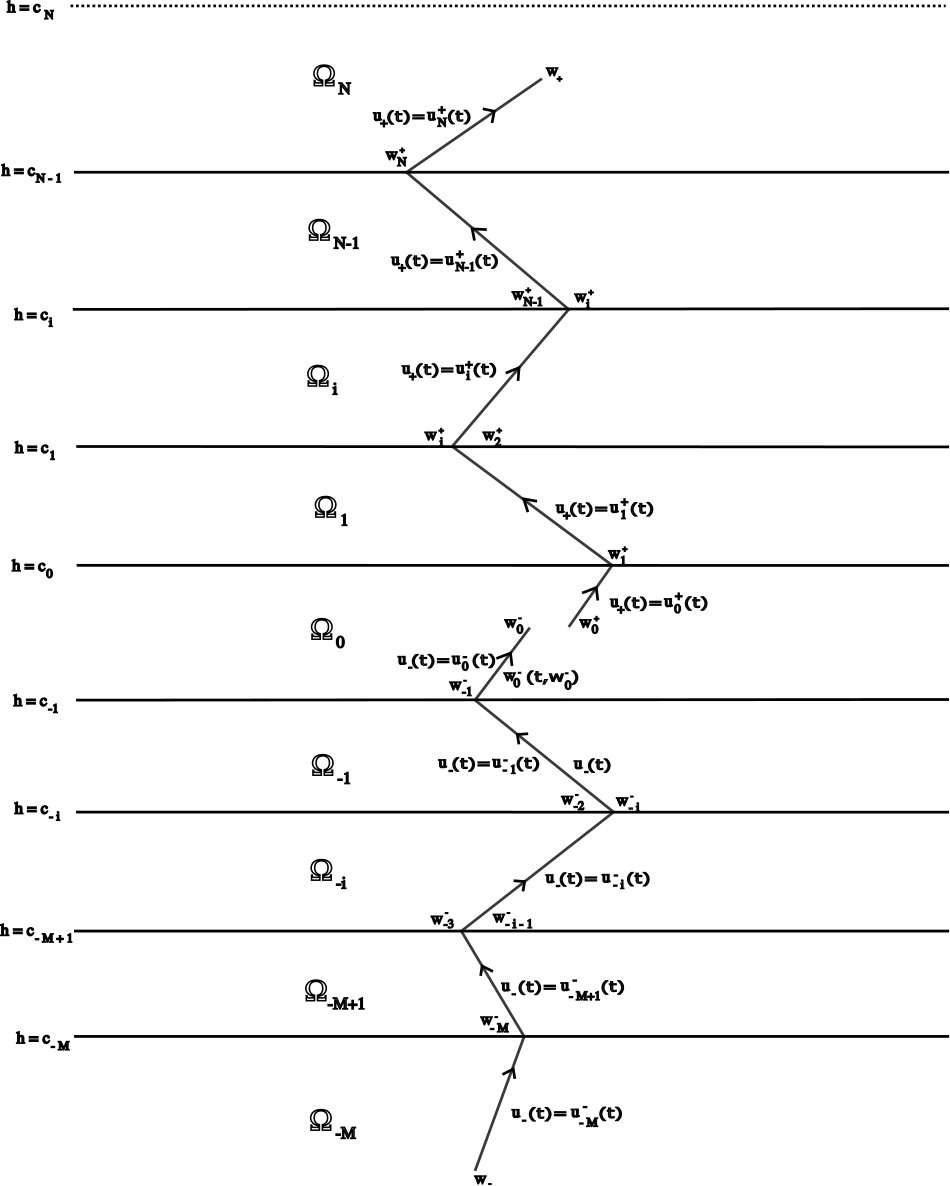 Figure 1
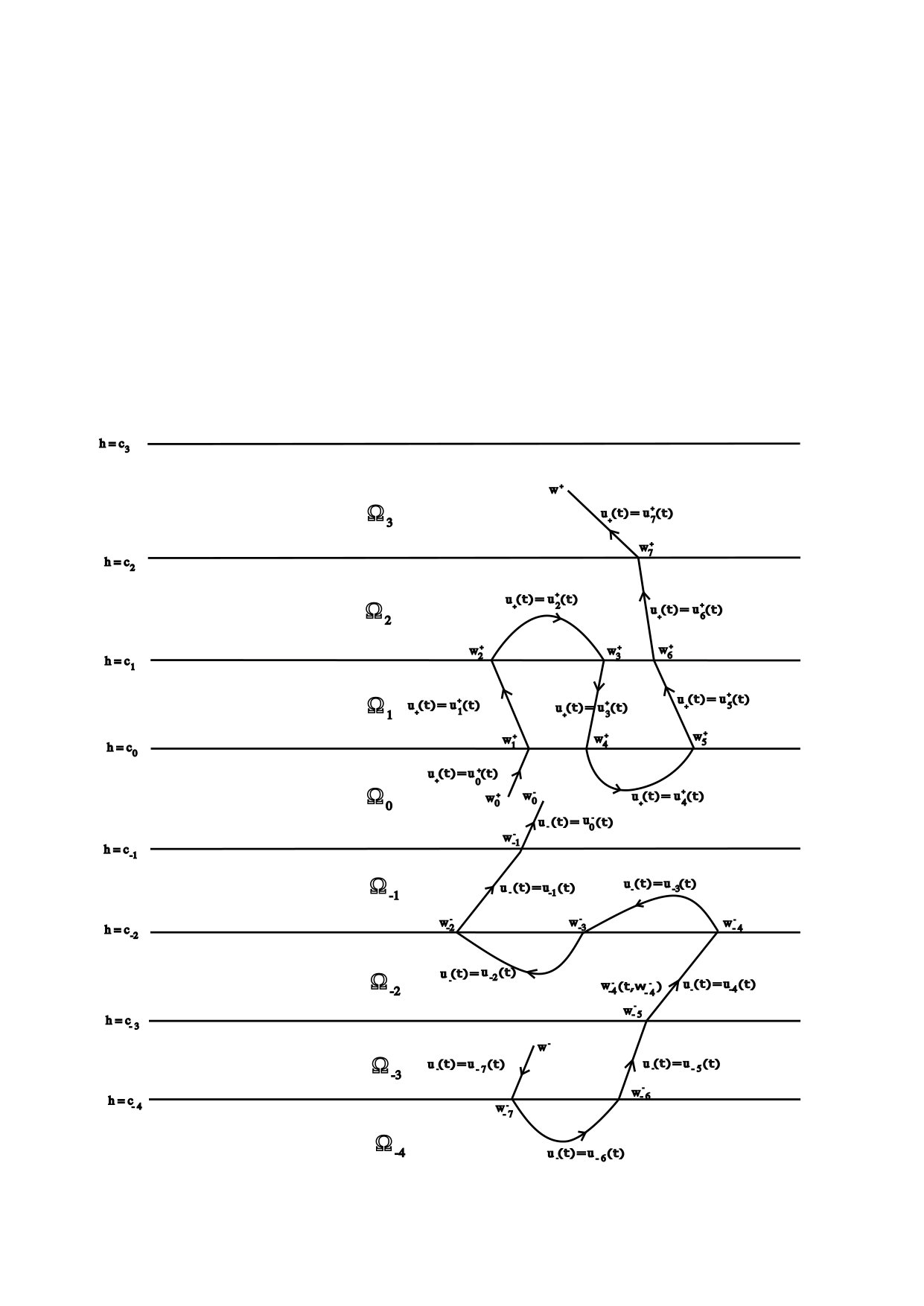 Figure 2
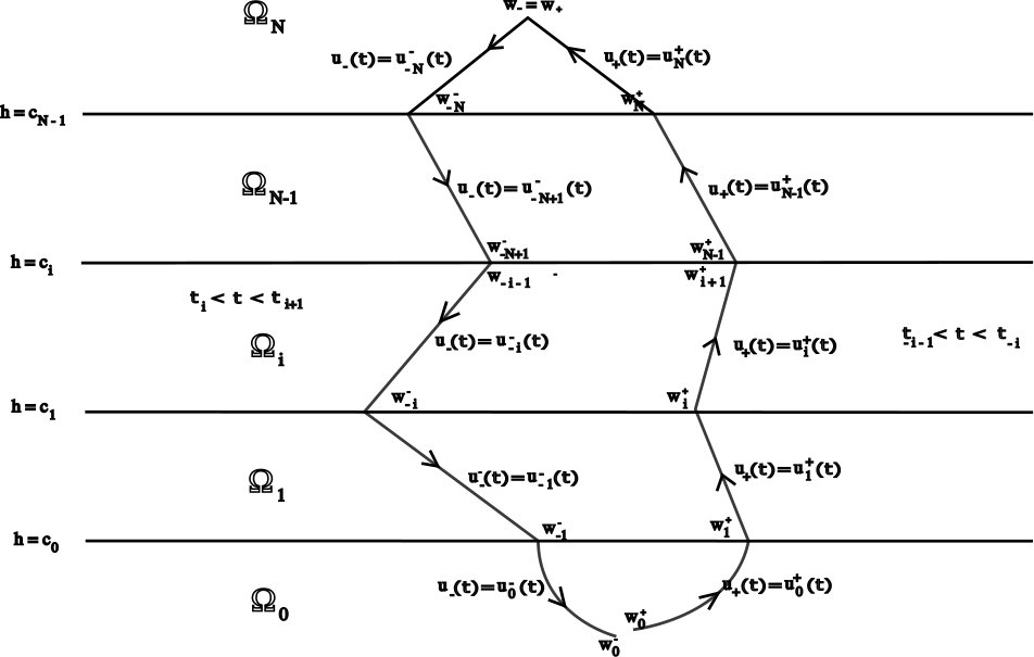 Figure 3
Peer Reviews
No public reviews on file for this paper yet. If you reviewed it on a platform where reviews are public (OpenReview, ICLR, NeurIPS, ICML), you can paste yours below so the community can read it here.
Videos
No videos yet. Explain this paper in a talk, walkthrough, or lecture? Add one.
Taxonomy
TopicsDifferential Equations and Numerical Methods · Nonlinear Differential Equations Analysis · Mathematical and Theoretical Epidemiology and Ecology Models
Heteroclinic Solutions in Singularly Perturbed Discontinuous Differential Equations
Flaviano Battelli
Department of Industrial Engineering and Mathematics
Marche Polytecnic University
Ancona - Italy
Michal Fečkan
Department of Mathematical Analysis and Numerical Analysis
Comenius University in Bratislava
Mlynská dolina, 842 48 Bratislava – Slovakia
and Institute of Mathematics, Slovak Academy of Sciences
Štefánikova 49, 814 73 Bratislava – Slovakia Partially supported by the National Natural Science Foundation of China (12161015), the Slovak Research and Development Agency under the contract No. APVV-18-0308 and by the Slovak Grant Agency VEGA No. 1/0084/23 and No. 2/0127/20
JinRong Wang
Department of Mathematics
Guizhou University, Guiyang
Guizhou 550025 – China
Abstract
We derive Melnikov type conditions for the persistence of heteroclinic solutions in perturbed slowly varying discontinuous differential equations extending to these equations similar results for continuous differential equations.
Key Words: discontinuous differential equations; heteroclinic solutions; Melnikov conditions; persistence.
1 Introduction
In recent years there has been a great deal in the study of singularly perturbed equations such as
[TABLE]
where and are sufficiently smooth functions. To the best of our knowledge this study started with remarkable papers by Tichonov [24], Vasil’eva et al. [25, 26]. All these results concern the behaviour of the solutions of (1.1) on a finite time scale. Later, Hoppensteadt [15, 16] extended the result on an infinite time scale. Then Fenichel [12] developed his geometric singularly perturbed theory that has been widely used by other authors as, for example, Szmolyan [23]. These last results essentially prove that the component of the solution is asymptotic to invariant manifolds, sometimes called centre manifolds, described by equations like (the case is allowed). In [18] a combination of the Melnikov method and geometric singular perturbation theory is presented. This approach has been then extended in [14] to investigate a mechanism of chaos near resonances both in the dissipative and the Hamiltonian context of differential equations.
The basic starting point for this kind of results is that, for all the frozen equation
[TABLE]
has hyperbolic fixed points, say , that are bounded functions of together with their derivatives, and solutions , defined for and , resp., such that
[TABLE]
uniformly with respect to and there exists such that . Hence, for the frozen equation (1.2) has a heteroclinic orbit connecting to . Note that in [6, 7, 20] it is also assumed that are bounded together with their derivatives. However, in Lemma 4.2, we prove that this condition is automatically satisfied when are bounded together with their derivatives and (1.3) holds. The proof of this result is rather technical and may be skipped at a first reading of this paper.
Other relevant results concerning (1.1) appeared in [6, 7, 8, 17, 20]. In [17], the second order equation with slowly varying coefficients
[TABLE]
is studied, where is a , -periodic function, such that . When and , (1.4) has the heteroclinic solution
[TABLE]
However this heteroclinic solution is broken when . In [17] it has been proved that if has a transversal intersection with at , i.e. and , then equation (1.4) has a heteroclinic solution. Writing
[TABLE]
equation (1.4) reads:
[TABLE]
where
[TABLE]
and . This solution is a part of a family of solutions such that
[TABLE]
and it can be proved that the transversality condition on corresponds to the fact that the real-valued function
[TABLE]
where is a suitable vector, has a simple zero at .
In Theorem 6.2, we extend these results, as far as the asymptotic behaviour of the -component of the solution is concerned, to discontinuous differential equations that is a differential equation which is described in different ways according to the region the solutions belong to. The first difference with the continuous case is that the way how passes from one domain into another is important. In this paper we assume that intersects transversally the boundary of the domain when they pass from the domain into another (see assumption in Section 2).
Problems like the above where is, instead, a family of periodic solutions depending on some further parameters and , have been studied in [27, 4, 5]. Note that, in [27], is replaced by and it is assumed that system
[TABLE]
has a one-parameter family of periodic solutions with period being in and it is because of the -dependence of the perturbed equation that the extra variable has been introduced. Then a vector valued function is constructed, that they called subharmonic Melnikov function, which is a measure of the difference between the starting value and the value of the solution at the time in a direction transverse to the unperturbed vector field at the starting point and proved that periodic solutions of the perturbed vector field arise near the simple zeros of . In [5] this result concerning the existence of periodic solutions has been extended to discontinuous systems of differential equations as the one we consider here.
Now, let us be more precise and give the definition of the discontinuous differential equation we are studying in this paper.
Let be a function, , with bounded derivatives, , , be -functions, bounded on together with their derivatives, and be real numbers. By discontinuous differential equation we mean an equation like
[TABLE]
where , , , and
[TABLE]
It is assumed that the equation
[TABLE]
has a hyperbolic fixed point [resp. ] together with continuous, piecewise solutions, , , , , such that
[TABLE]
uniformly with respect to , and
[TABLE]
for any , .
Here we used the shorthand for , when , and , when . We will use such a shorthand throughout the whole paper.
Note that (1.10) implies that intersects transversally the set
[TABLE]
at . Then we look for solutions of (1.7) such that
[TABLE]
Note that, from (1.10) it follows that, for any , the set , , , is an hypersurface in a ball around whose radius does not depend on . We emphasize that (1.10) is all that we need on for our analysis.
To prove the existence of solutions of (1.7) satisfying (1.11) we use Lyapunov-Schimtd method, together with a combination of singularly perturbed analysis and a technique for discontinuous dynamical systems, to construct a bifurcation function whose zeros are associated to solutions of the perturbed equation whose -component satisfies (1.11). This is the content of Theorem 6.2 where we prove that if a certain generic condition is satisfied then there is a manifold of such solutions.
According to (see Section 2) are normally hyperbolic invariant manifolds for the unperturbed system , . From [1, 22] these manifolds perturb to invariant manifolds such that
[TABLE]
From Remark 6.3 it follows that is asymptotic to the manifold as and to as . Hence, behaves as a heteroclinic solution of equation (1.7) connecting the invariant manifold to .
The problem studied in this paper has been motivated by [28], where existence and bifurcation theorems are derived for homoclinic orbits in three-dimensional flows that are perturbations of families of planar Hamiltonian system. In this paper we study the problem of persistence of bounded solutions in the discontinuous case (1.7) where , , all functions considered are sufficiently smooth and is a small parameter, assuming the existence of such an orbit in the unperturbed equation (1.9).
Then in Section 7 we apply Theorem 6.2 to extend [17, Theorem 1] to the discontinuous equation (1.7). Following [6] we derive a bifurcation function characterizing the persistence of homoclinic solutions of (1.7) from a generic homoclinic solution of the unperturbed system (1.6). It can be easily checked that the results of this paper easily extend if we replace with (with the same ). In this case the unperturbed system will be
[TABLE]
The next step is the study of a degenerate case where, for any the unperturbed discontinuous equation (1.6) has a piecewise solution heteroclinic to the hyperbolic fixed points . We plan to perform this study in a forthcoming paper as it is necessary to go into a deeper analysis of the bifurcation function.
We now briefly sketch the content of this paper. In Section 2 we provide basic assumptions and define the piecewise smooth heteroclinic solution of the unperturbed system. In Section 3 we recall the definition of exponential dichotomy and extend this notion to discontinuous, piecewise linear, systems with a jump at some points. We also extend to these systems some results concerning existence of bounded solutions on either and . In our opinion, these results are theirselves interesting as they give the form of the projection of the dichotomy of a linear discontinuous system. Although this is an important point in the proof of Theorem 6.2, we think that the proofs in this section can be skipped at a first reading.
Next, in Section 4, we construct families of bounded solutions and describe them in terms of some parameters. These solutions are continuous and piecewise smooth and give the bounded solutions we look for, when they assume the same value at . Then, after having defined the variational equation in Section 5, in Section 6 we study the joining condition at which is the bifurcation condition and give a Melnikov-type condition assuring that the bifurcation equation has a manifold of solutions. Finally, in Section 7 we first state some general facts concerning two-dimensional discontinuous equations depending on a slowly varying parameter and give an example of application of the main result of this paper. In Section 8 we give a hint on a possible extension of the example.
In the whole paper we will use the following notation. Given a vector or a matrix with , (resp. ) we denote the transpose of (resp. ).
2 Notation and basic assumptions
Let be a bounded domain,
[TABLE]
be real numbers and be a -functions, , with bounded derivatives. For , we set
[TABLE]
where we set for simplicity, and let be -function, bounded together with their derivatives in . We are looking for solutions of equation
[TABLE]
which are contained in a compact subset of . Hence it is not restrictive to assume that . So, from now on, we suppose .
First we give the definition of solutions of equation (2.1) we are considering in this paper
Definition 2.1**.**
A continuous, piecewise smooth function is a solution of equation (2.1) on intersecting transversally the sets , , if there exist and such that the following conditions hold for (note that we set )
* for and for ;*
;
, for and , for .
Similarly, a continuous, piecewise smooth function is a solution of equation (2.1) on intersecting transversally the sets , , if there exist and such that the following conditions hold for any :
* for and for ;*
;
, for and , for .
In this paper we assume that continuous, piecewise smooth solution and of equation (2.1) exist, for , resp. , such that the following conditions also hold.
and their derivatives are bounded functions and belong to an open and bounded subset such that .
There exist smooth and bounded functions and , such that
[TABLE]
for any and
[TABLE]
uniformly with respect to .
For any , and have eigenvalues with negative real parts and eigenvalues with positive real parts, counted with multiplicities and there exists such that all these eigenvalues satisfy
[TABLE]
There exists such that .
Remark 2.2*.*
From it follows that is a continuous, piecewice solution of such that
[TABLE]
Moreover, from it follows that, for :
[TABLE]
that is
[TABLE]
Similarly we see that
[TABLE]
So are a kind of transversality assumption on the solutions .
ii) All results in this paper can be generalised to the case where the solutions exit transversally and enter into either or transversally in the sense that (1.10) holds at the intersection points of the solution with the boundary of . More precisely suppose, to fix ideas, . Then we assume the following (see Fig. 2). There exists such that given then is either or and for we have
[TABLE]
Moreover
[TABLE]
for any .
A similar generalization can be made for and all other assumptions are changed accordingly.
Another possible generalization is the homoclinic case. This is the case, for example, where and assumptions are changed to the following where we write instead of (see Fig. 3):
for and for ;
and ;
, and , for .
where, we set for simplicity, .
We have the following
Lemma 2.3**.**
For , , let , . Then and are -functions bounded together with their derivatives.
Proof.
We know that is and bounded together with its derivatives. Now,
[TABLE]
Hence is and bounded since so are , and . Next, from
[TABLE]
and the fact that is bounded, we see that exists such that . Then, differentiating we see that
[TABLE]
is bounded. More arguments of similar nature show that all derivatives of are bounded.
Suppose now that is bounded with its derivative. Then, since
[TABLE]
we see that is a bounded function and a similar argument as before shows that the derivatives of are also bounded. The proof that is a function bounded with its derivatives for any is similar. ∎
Let . For , let be the solution of such that . Similarly, for let be the solution of such that . Then
[TABLE]
where, for simplicity, we set and
[TABLE]
and similarly,
[TABLE]
Here we emphasize a convention that we will use throughout the whole paper. When we use the index , such as in or , we always mean , (sometimes also ) while, when we use the index , as in or , we always mean (sometimes also ).
3 Exponential dichotomy for piecewise discontinuous systems
A basic tool in this paper is the notion of exponential dichotomy, whose definition we recall here. Let be either , or and , , be a continuous matrix. We say that the linear system
[TABLE]
has an exponential dichotomy on if there exist a projection and constants and such that the fundamental matrix of (3.1) satisfying , when , or when , satisfies
[TABLE]
In this section we extend the definition of exponential dichotomy to systems with discontinuities. To allow more generality we consent the solutions to have jump discontinuities at the discontinuity points of the coefficient matrix.
So, let be real numbers, be invertible matrices and , be a piecewise continuous matrix with possible discontinuity jumps at , that is
[TABLE]
where are continuous matrices. Note that is continuous for , , and right-continuous at , with possible jumps at given by the matrix . For we consider the linear, discontinuous, system
[TABLE]
Similarly, if and
[TABLE]
where are continuous matrices, we consider, for , the linear, discontinuous, system
[TABLE]
Note that is continuous for , , left-continuous at , with possible jumps at , given by the matrix .
Remark 3.1*.*
i) As a matter of facts, for , we will consider
[TABLE]
and similarly for . This may cause a duplicate definition of at , however it will be always clear which among will be taken into account at that point.
ii) The results of this section will be applied to the linear system where is given by
[TABLE]
Note that, being continuous for , is continuous for , with jump discontinuities at . More precisely
[TABLE]
Without loss of generality we may assume that , so in the remaining part of this section we will take .
Let be the fundamental matrix of the linear systems
[TABLE]
on , that is , , and . The fundamental matrix of (3.3), where , is given by the (discontinuous) invertible matrix
[TABLE]
that is
[TABLE]
Similarly, the fundamental matrix of (3.3), where , is given by the (discontinuous) invertible matrix
[TABLE]
Note that is continuous for and right-continuous at and is continuous for and left-continuous at .
It is clear that , for , , , for , , , the identity matrix, and
[TABLE]
Actually we can write
[TABLE]
since is right-continuous and is left-continuous. Then, from (3.7) and (3.8) we see that
[TABLE]
and, similarly,
[TABLE]
Remark 3.2*.*
i) Let be a fixed number. For , is the right-continuous solution of
[TABLE]
Indeed, it is obvious that for , and that , since . Moreover , since is right-continuous at any .
Similarly, for and any fixed , is the left-continuous solution of
[TABLE]
ii) As is right-continuous at it is also clear that satisfies
[TABLE]
and, similarly, satisfies
[TABLE]
We have the following
Lemma 3.3**.**
Suppose that the linear system
[TABLE]
has an exponential dichotomy on (resp. ) with constant , exponent and projection (resp. ). Then, the linear system (3.3) (resp. (3.5)) with as in (3.2) (resp. (3.4)) has an exponential dichotomy on , (resp. ) with the same exponent , constant and projection
[TABLE]
Proof.
As is right continuous at , for we have
[TABLE]
since is the fundamental matrix of on . Similarly we see that
[TABLE]
for . Being compact and piecewise continuous with right and left limits at the discontinuity points, there exists such that
[TABLE]
for . Finally, for , we have, using right-continuity of :
[TABLE]
proving the result for with . A similar argument works when . The Lemma is proved. ∎
The following result characterises , resp. , in terms of bounded solutions of system (3.3), resp. (3.5), extending to the discontinuous case a simular result for continuous equations.
Lemma 3.4**.**
Let be either as in (3.2) or (3.4). Suppose that the condition of Lemma 3.3 hold and let be as in (3.15). Then if and only if the solution of the discontinuous system (3.3) such that is bounded for . Similarly, if and only if the solution of the discontinuous system (3.3) such that is bounded for .
Proof.
If we have
[TABLE]
that is the solution of (3.3) starting from is bounded. Vice versa, suppose that is a solution of (3.3) bounded on . We have
[TABLE]
as . Then and hence . By a similar argument we prove the thesis when is concerned. ∎
We conclude this section with the following
Lemma 3.5**.**
Let , , be invertile matrices and be a bounded integrable function for , (resp. ). Suppose the condition of Lemma 3.3 hold and set
[TABLE]
where is as in (3.15) and is a fixed number. Then, for any (resp. ) the linear inhomogeneous system
[TABLE]
with , [resp.
[TABLE]
when ] has the unique right-continuous, [resp. left-continuous when ] bounded solution
[TABLE]
[resp.
[TABLE]
if ]. Moreover such a solution satisfies
[TABLE]
if [resp.
[TABLE]
if ].
Proof.
We only give the proof for , the proof for being similar. We prove uniqueness, first. Suppose that are two solutions of (3.16), right-continuous and bounded for . Then is a right-continuous, bounded solution of
[TABLE]
Then, as we have observed in Remark 3.2-i), , so:
[TABLE]
from which we get
[TABLE]
as , since is bounded. This proves that and then . Hence we have uniqueness. To show the existence we observe that the function given in (3.17) is right-continuous, bounded for (and hence also for ) and satisfies (3.16). Finally, from (3.17) we get:
[TABLE]
from which (3.19) easily follows. ∎
4 Bounded solutions on the half lines
In this section we prove the existence of continuous solutions , with , of the perturbed linear system (1.7) such that
[TABLE]
where is a sufficiently small positive real number. By a similar argument we can also prove the existence of continuous solutions of (1.7), with , such that
[TABLE]
From it follows that the number of the eigenvalues of , with negative (and then also positive) real parts, counted with multiplicities, is independent of . Moreover it also follows that all eigenvalues are bounded functions of . Indeed, since is bounded, the matrix is invertible for , sufficiently large and independent of . Hence all eigenvalues have to satisfy . The same arguments work as far as the eigenvalues of are concerned.
As in , let be the number of eigenvalues with negative real parts, counted with multiplicities, of the matrix and be any positive number strictly less than , where are the eigenvalues of . According to [11] the system has an exponential dichotomy on with exponent and (spectral) projection
[TABLE]
where is the residual of the meromorphic function at and is a closed curve that contains in its interior all eigenvalues of with negative real parts, but none of those with positive real parts. Hence , for some . Similarly we see that has an exponential dichotomy on with exponent and projection such that , for some .
Now, from we know that
[TABLE]
uniformly with respect to .
Let , and take . From the roughness of exponential dichotomies (cfr. [11, Proposition 2, p. 34]) the linear systems
[TABLE]
and
[TABLE]
have an exponential dichotomy on , resp., uniform with respect to , with projections , resp. , of rank , constant and exponent . Moreover, according to [20, Proposition 2.3], it can be assumed that, for sufficiently small it results: , and in this case the projections are smooth with respect to . Note that, and are equivalent to
[TABLE]
For , , let , [resp. ] be the fundamental matrix of
[TABLE]
in resp., that is
[TABLE]
resp.
[TABLE]
We have the following
Lemma 4.1**.**
For any the linear system
[TABLE]
resp.
[TABLE]
has an exponential dichotomy on , resp. , with exponent , constant independent on and projections
[TABLE]
In particular, if , resp. , then , resp. , and .
Proof.
As is the fundamental matrix of (4.4) in , the fundamental matrix of (4.1) on is
[TABLE]
while the fundamental matrix of (4.4) on is
[TABLE]
Then
[TABLE]
So we get, for :
[TABLE]
and similarly
[TABLE]
Hence (4.4) has an exponential dichotomy on with projection , constant and exponent . If the proof is finished. Moreover if we have
[TABLE]
If , for let
[TABLE]
Then satisfies
[TABLE]
with . Hence
[TABLE]
So, using :
[TABLE]
where is an upper bound for . Setting we get
[TABLE]
Integrating on we get, since , . Hence
[TABLE]
and then
[TABLE]
where
[TABLE]
Note that is independent of . Finally, for we have
[TABLE]
By a similar argument we prove that
[TABLE]
for .
The proof that (4.5) has an exponential dichotomy on , with projection , exponent and a constant independent of is similar. ∎
From the proof of the parametric stable (resp. unstable) Theorem (see [19, p. 18]) it follows that, all solutions of such that (resp. ) can be obtained as fixed points of a uniform contraction, with respect to , on the space of bounded functions. It follows, then, that these solutions are bounded together with their derivatives.
The following Lemma states that the bounds for , and their derivatives with respect to can be taken independent of . Due to its technical character the proof of Lemma 4.2 is postponed in the Appendix.
Lemma 4.2**.**
Assume . Then and its derivatives with respect to are bounded uniformly with respect to , on . Similarly, and its derivatives with respect to are bounded, uniformly with respect to , on .
From [6, Theorem 2] we get the following
Theorem 4.3**.**
Suppose that hold and let be such that . Then there exist , and such that for and , with , , and , system
[TABLE]
has a unique solution , such that
[TABLE]
Moreover,
[TABLE]
as , uniformly with respect to . Similarly for and such that , system
[TABLE]
has a unique solution , such that
[TABLE]
Moreover
[TABLE]
as , uniformly with respect to . Moreover, for any , the function
[TABLE]
is of class and, for , the -th order derivatives are bounded above in absolute value by , where is a suitable constant. Similarly, for , the map
[TABLE]
is of class and the -th order derivatives are bounded above in absolute value by , where is a suitable constant.
Proof.
In [6] the equations are considered for or and instead of it is considered . To obtain the result as in Theorem 4.3 for , (resp. ) we take (resp. ) and apply [6, Theorem 1] with , resp. , instead of . Suppose, to fix ideas, that . We know that (4.1) has an exponential dichotomy on with projection and, from Lemma 4.2 that and its derivatives with respect to are bounded uniformly with respect to . From [6, Theorem 1] we obtain then a unique solution
[TABLE]
of (1.7) such that
[TABLE]
and
[TABLE]
as , uniformly with respect to . Setting
[TABLE]
we see that satisfies
[TABLE]
and
[TABLE]
since . A similar argument works for . Finally, we observe that, although in [6] it is not explicitly stated that (4.7), (4.9) hold uniformly with respect to , this fact easily follow from [6, (20)-(23)] and . ∎
Remark 4.4*.*
According to assumption , are normally hyperbolic manifolds for the system
[TABLE]
These manifolds perturb to normally hyperbolic invariant manifolds for the system
[TABLE]
(see, for example, [1, 22]). Let be the solution of such that .
It follows from [9, Theorem 1] that, for and sufficiently small, with and , there exists a unique solution of
[TABLE]
such that
[TABLE]
and .
As and uniformly with respect to we conclude that
[TABLE]
where is sufficiently large. From continuous dependence we see that the above estimate holds with instead of , provided is sufficiently small, and then
[TABLE]
for some and . As a consequence the solutions given in Theorem 4.3 satisfy
[TABLE]
Similarly we see that
[TABLE]
In the remaining part of this section we extend the solutions obtained in Theorem 4.3 to continuous, piecewise solutions of (1.7) in resp. . We have the following
Theorem 4.5**.**
There exist , bounded -functions
[TABLE]
and continuous, piecewise solutions of (1.7)
[TABLE]
defined for and resp., such that
[TABLE]
(, ) uniformly with respect to and
[TABLE]
where . Moreover
[TABLE]
and
[TABLE]
uniformly with respect to .
Proof.
Suppose . Since , from (4.7) we see that
[TABLE]
as (uniformly with respect to ). Hence , provided is sufficiently small and uniformly with respect to . Then can be extended to a solution of
[TABLE]
which is defined for and such that
[TABLE]
as , uniformly with respect to . Note that
[TABLE]
as , uniformly with respect to , since and uniformly with respect to . Now, from and the implicit function theorem it follows that there exists a -function , bounded together with its derivatives, such that
[TABLE]
provided is sufficiently small, uniformly with respect to . Next, from the continuous dependence on the data, we see that the system
[TABLE]
has a unique solution , defined for , such that
[TABLE]
(where ) for sufficiently small and the following holds
[TABLE]
as , uniformly with respect to . Now, as
[TABLE]
from the implicit function theorem we see that a -function , bounded together with its derivatives, exists such that
[TABLE]
uniformly with respect to and the following holds:
[TABLE]
Proceeding this way we construct the solution with the properties stated in the Theorem. A similar argument works for . The proof is complete ∎
Remark 4.6*.*
According to Theorem 4.5 we have
[TABLE]
Differentiating the above equalities with respect to , , at we obtain a formula for the derivatives
[TABLE]
However we have to distinguish when or (resp. or ). For example if , is the solution of and then, differentiating (4.12) with respect to , we get, with :
[TABLE]
Vice versa, when , is the solution of and then
[TABLE]
Similarly we get
[TABLE]
and
[TABLE]
We will use this remark in the next section.
5 The variational equation
Let . For fixed we define linear operators as follows:
[TABLE]
Note that (recall that , ):
[TABLE]
We have the following:
Proposition 5.1**.**
For any and , are invertible linear maps. Moreover is a solution of
[TABLE]
which is for , bounded for and can be assumed to be right-continuous at . Similarly is a solution of
[TABLE]
which is for ,bounded for and can be assumed to be left-continuous at .
Proof.
First we prove that is invertible. If , there is nothing to prove since . So, suppose that and . Then
[TABLE]
where . Hence:
[TABLE]
But then since
[TABLE]
Next, is a continuous, piecewise , solution of the differential equation
[TABLE]
Hence, for , when , or when , we have
[TABLE]
Differentiating with respect to we get, for the same values of :
[TABLE]
and then,
[TABLE]
where we write for simplicity
[TABLE]
Now, from Remark 4.6 we see that
[TABLE]
Hence
[TABLE]
where
[TABLE]
Taking , we see that is a solution, for of (5.2) where is as in (5.1).
Following a similar argument we see that is a solution, for of (5.3) where is as in (5.1).
Finally we prove that is bounded for . It is enough to prove this for . From Theorem 4.3 we know that is a solution of
[TABLE]
such that
[TABLE]
So, is a bounded solution of the linear system
[TABLE]
whose fundamental matrix on is . According to Lemma 4.1 (5.7) has an exponential dichotomy on with projection and exponent . Then we have . But then is bounded for because is the space of initial conditions of solutions of that are bounded for . A similar argument shows that is bounded for . The proof is complete. ∎
In the next proposition we show that is a nontrivial bounded solution of (5.2) for (resp. (5.3) for ).
Proposition 5.2**.**
For , resp. , the function
[TABLE]
resp.
[TABLE]
is a solution of (5.2) (resp. (5.3)) bounded on (resp, ) where is as in (5.1).
Proof.
We already know that satisfies (5.2), for and (5.3) for , . We prove that . We have
[TABLE]
The proof is complete. ∎
6 The Melnikov condition
First we recall that is the projections of the exponential dichotomy on , of the linear system (4.1) with constant and exponent . Then, from Lemma 4.1, we see that (4.4) has an exponential dichotomy on with exponent and projection
[TABLE]
the equality following from (3.9) and .
Similarly, the linear system (4.5) has an exponential dichotomy on with exponent and projection
[TABLE]
where
[TABLE]
and
[TABLE]
are the fundamental matrix of , where is as in (3.6).
From Lemma 3.3–3.4 and (6.1)-(6.2) we obtain the following
Proposition 6.1**.**
For any , the discontinuous linear system (5.2) (resp. (5.3)) has an exponential dichotomy on , (resp. ) with projections , resp. , given by
[TABLE]
Moreover (resp. ) is the space of initial conditions of solutions of (5.2), resp. (5.3), right-continuous, when (resp. left-continuous, when ) and bounded on , (resp, on ).
For simplicity we write .
We assume the following condition holds:
.
From Proposition 5.2 we see that so
[TABLE]
Next, from we know that and , hence .
Let be such that . Without loss of generality we assume that is an orthonormal set.
The purpose of this section is the to prove the following
Theorem 6.2**.**
Suppose that hold. Suppose further that the matrix has rank . Then there exists and such that for system (1.7) has a -dimensional manifold of continuous, piecewise solutions such that
[TABLE]
as .
Proof.
First, we apply Lemma 3.5 to obtain another expression of (resp. ). We know that, for ,
[TABLE]
is a bounded and continuous solution of the differential equation
[TABLE]
that we write:
[TABLE]
where has been defined in (3.6) and
[TABLE]
Note that
[TABLE]
and, according to ,
[TABLE]
Hence, for sufficiently small there exist -functions such that
[TABLE]
for any and uniformly with respect to . Then
[TABLE]
and
[TABLE]
According to Lemma 3.5, with , we see that
[TABLE]
where
[TABLE]
Note that
[TABLE]
as , uniformly with respect to . We prove the following
Claim: For sufficiently small, the map , with from into is linearly invertible.
Indeed, for the above map reduces to
[TABLE]
where
[TABLE]
Hence
[TABLE]
Now, from Proposition 5.1 we know that, for any ,
[TABLE]
is a right-continuous solution, bounded on , of
[TABLE]
the last relation following differentiating the equality
[TABLE]
with respect to at (see Theorem (4.3)). In particular we have for any (see Remark 3.2). From Lemma 4.1 it follows that the linear system (4.4), with , has an exponential dichotomy on with projection (see also (3.9))
[TABLE]
as . Hence
[TABLE]
As a consequence
[TABLE]
So, is a right-continuous solution, bounded on
[TABLE]
for any . Now, with reference to Lemmas 3.3, 3.5 with , we have
[TABLE]
Hence is a bounded solution of
[TABLE]
From Lemma 3.5, equation (3.17), we get then, for any , using again the right-continuity of :
[TABLE]
So,
[TABLE]
Hence is an isomorphism from into and the Claim is proved.
Similarly we see that
[TABLE]
where
[TABLE]
and
[TABLE]
Again we see that
[TABLE]
as , uniformly with respect to and the map from into is linearly invertible.
From (6.4)-(6.5) we get, for sufficiently small
[TABLE]
Hence the system
[TABLE]
is equivalent to
[TABLE]
Let
[TABLE]
Differentiating with respect to at , and using , , we see that, for , we have
[TABLE]
and for :
[TABLE]
Then
[TABLE]
and similarly
[TABLE]
As a consequence, on account of , (6.7) reads:
[TABLE]
where and , uniformly wth respect to . Since and are linearly invertible we see that and hence (6.7) reads:
[TABLE]
where and , uniformly wth respect to . Now we can write and hence
[TABLE]
provided is sufficiently small. Similarly, for is sufficiently small, . In particular the map from into , and from into are linearly invertible. Then, setting
[TABLE]
(6.8) can be written as
[TABLE]
where and , uniformly with respect to . Now the map is a linear map from into whose kernel is which, by assumption , is -dimensional.
Let be a complement of in , so that
[TABLE]
Note that and . Recall that we assumed that is orthonormal. Then, let be the orthogonal projection such that and . Since and is orthonormal we get
[TABLE]
Hence we replace (6.9) with
[TABLE]
Since , for any
[TABLE]
is essentially a system of equations in the variables such that, when , has the solution
[TABLE]
The Jacobian matrix at this point is
[TABLE]
where is the invertible linear map given by . We have
[TABLE]
hence, for and sufficiently small (6.11) has a -dimensional manifold of solutions
[TABLE]
where
[TABLE]
Note also that
[TABLE]
uniformly with respect to . Then we plug this solution in the third equation in (6.10) and obtain the system of equations
[TABLE]
Let
[TABLE]
We have , and
[TABLE]
Hence from the Implicit Functions Theorem the existence follows of such that for any there exists a -dimensional submanifold of such that when we have . For , we take
[TABLE]
and , so that
[TABLE]
Then
[TABLE]
with satisfies the conclusion of the Theorem. The proof is complete. ∎
Remark 6.3*.*
i) According to Remark 4.4 we see that satisfies
[TABLE]
where do not depend on .
ii) We can replace the orthonormal basis of with any independent set such that
[TABLE]
Indeed, let be a scalar product on such that
[TABLE]
and let be an orthonormal basis of . Then an invertible matrix exists such that
[TABLE]
Hence
[TABLE]
that is has rank if and only if has rank .
We conclude this section giving another expression for that can be useful in the applications of Theorem 6.2.
Proposition 6.4**.**
Let be the -function defined in (2.2) and let . Then
[TABLE]
where
[TABLE]
Hence, the Melnikov conditon in Theorem 6.2 reads
[TABLE]
where is as in (6.12) with instead of .
Proof.
As is a bounded solution of
[TABLE]
where is as in (3.6) with , and
[TABLE]
from to Lemma 3.5, equation (3.18), with we get:
[TABLE]
Taking the and using , we get
[TABLE]
that is
[TABLE]
Similarly
[TABLE]
Now, since
[TABLE]
for any we get
[TABLE]
Hence, for any we have:
[TABLE]
where is as in (6.12) with instead of . The proof is complete. ∎
The adjoint system to (5.2) and (5.3) is given by [3]
[TABLE]
where .
It is easy to check that, if , the function defined in (6.12) is a bounded solution of (6.15) for . We prove that if then is a basis for the space of the bounded solutions of (6.15). Indeed, the fundamental matrix of (6.15) on is , and the fundamental matrix of (6.15) on is . As a consequence (6.15) has an exponential dichotomy on and with projections and respectively. So, the space of bounded solutions of (6.15), for , are those whose initial conditions belong to
[TABLE]
Then the dimension of the space of solutions of (6.15), bounded on , is and span this space.
Now suppose that and are bounded solution on of (5.2)-(5.3) and (6.15) resp., both continuous for . For we have
[TABLE]
Moreover
[TABLE]
Thus we conclude that is constant on (see also [21]).
7 An example
An interesting application of Theorem 6.2 is when that is when
[TABLE]
This condition is trivially satisfied when since in this case . Moreover, when , we also have and hence
[TABLE]
In this section we consider examples of applications of Theorem 6.2 with , and . First we prove some general facts concerning two-dimensional differential equations depending on a slowly varying variable. So the system is
[TABLE]
Suppose is a piecewise smooth solution of (7.2) for satisfying assumptions . To write the Melnikov condition (6.13), that in this case reads
[TABLE]
we need to know the (unique) bounded solution of the adjoint system (6.15).
Let
[TABLE]
and, again, .
We prove the following
Proposition 7.1**.**
Let , as in (5.1), with and
[TABLE]
Then the space of bounded solution of the adjoint variational system are of the form
[TABLE]
where is arbitrary and
[TABLE]
Proof.
First we show that constants satisfying (7.3) exist. Indeed recall that for any
[TABLE]
where , and then
[TABLE]
for some , since both vectors are orthogonal to . In a similar way we see that constants satisfying (7.3) for exist.
Next, using :
[TABLE]
Hence
[TABLE]
for any . Moreover
[TABLE]
Finally, we prove that is bounded. As the adjoint system has an exponential dichotomy on , resp. , with projections , resp. , it is enough to prove that
[TABLE]
the last equality following from (7.1). But
[TABLE]
and then is bounded concluding the proof of the Proposition. ∎
Remark 7.2*.*
i) From (7.3) we have
[TABLE]
and then
[TABLE]
and similarly
[TABLE]
Hence all ’s can be computed in terms of .
ii) Since and all , are invertible, we see that for all .
The case where all are equal is of particular interest, since in this case we can take and the Melnikov condition reads
[TABLE]
If, moreover, we have
[TABLE]
where .
We have the following
Proposition 7.3**.**
Equations (7.3) are satisfied with and , if and only if there exist such that
[TABLE]
Proof.
We have , for all , if and only if the following holds.
[TABLE]
We check that
[TABLE]
so that
[TABLE]
Then (7.6) is equivalent to :
[TABLE]
or else, as ,
[TABLE]
which is (7.5) with
[TABLE]
On the other hand, if (7.5) holds, taking the scalar product with we get
[TABLE]
that is
[TABLE]
and then (7.6) follows, given the equivalence between (7.6) and (7.8) ∎
Remark 7.4*.*
As is orthogonal to and is orthogonal to the tangent space to at , say , condition (7.5) is equivalent to the fact that belongs to .
For example, suppose
[TABLE]
where either or . Recalling that
[TABLE]
we get, omitting the argument for simplicity:
[TABLE]
and then (7.5) holds if and only if
[TABLE]
To give a specific example, consider the second order, discontinuous equation with slowly varying coefficients:
[TABLE]
where .
We prove the following
Proposition 7.5**.**
Let be -functions such that
[TABLE]
and let be a fixed number. Then equation (7.9) with has a family of -solutions defined for , resp., bounded together with their derivatives, such that and
[TABLE]
uniformly with respect to . Next, let and suppose that and exist such that
[TABLE]
Then and there exists such that for there exists a -function , such that , and a -solution of equation (7.9) with , bounded with its derivatives and such that
[TABLE]
Proof.
Writing , , equation (7.9) reads
[TABLE]
where
[TABLE]
Then and
[TABLE]
Note that
[TABLE]
is tangent to the manifold and (7.9) has the fixed points and .
Let (7.11)0 be equation (7.11) with and , , be solutions of (7.11)0 such that
[TABLE]
Multiplying (7.9) (with ) by and integrating from to we get
[TABLE]
hence, if , it satisfies
[TABLE]
It is easy to check that, for we have .
To simplify notation in the following we write for . Integrating (7.12) we get (see [13, eq. 2.266])
[TABLE]
where . Then, using and :
[TABLE]
Hence
[TABLE]
where
[TABLE]
We pause for a while to observe that is well defined if . This holds for sure if . However, if we need that
[TABLE]
We will consider this issue in Section 8.
As and its derivative are bounded on , so are and , Moreover, from (7.14) it follows that is in .
We have
[TABLE]
As
[TABLE]
for , we see that and do not change sign in . But, since for we have
[TABLE]
we see that . Moreover and and that . So
[TABLE]
and then
[TABLE]
As a consequence for and
[TABLE]
uniformly with respect to . From (7.12) we also see that and uniformly with respect to . In particular, for , are bounded, positive, functions and is strictly increasing from [math] to .
Now, we look for a (strictly) increasing solution of the second equation in (7.9) on . To this end we observe that, is a (strictly) increasing solution, on , of the second equation in (7.9) such that
[TABLE]
if and only if is a (strictly) increasing solution, on , of
[TABLE]
such that
[TABLE]
Since is equivalent to , from the previous part we conclude that the second equation in (7.9) has a unique strictly increasing solution such that
[TABLE]
the limit being uniform with respect to .
Then for any , equation (7.9) with has a pair of solutions , defined for and resp., such that are increasing in their interval of definition and
[TABLE]
uniformly with respect to .
Now, since and we get:
[TABLE]
So equation (7.9), with , has a solution heteroclinic to the fixed points and if and only if
[TABLE]
It is easy to check that
[TABLE]
and hence equation (7.9) has a solution heteroclinic to the fixed points and if and only if
[TABLE]
From (7.10) we see that equation (7.19) has a unique solution only for .
Then equation (7.11)0 has a unique solution asymptotic to as and to as only for and this solution breaks when (in the sense that it is no longer ). Since is tangent to the manifold and
[TABLE]
the Melnikov function reads:
[TABLE]
From Theorem 6.2 the existence follows of and such that for there exist a -function with and a solution of (7.11) such that
[TABLE]
∎
Remark 7.6*.*
Suppose that with . Then (7.10) reads:
[TABLE]
Note that for .
8 Concluding remark
The assumption can be slightly weakened. Indeed, suppose that
[TABLE]
where .
By uniqueness of analytical continuation, the function defined in (7.14) is a solution of the first equation in (7.5) (with ) for any value of for which has a meaning, that is such that
[TABLE]
Moreover to prove that as , uniformly with respect to , following the same argument of Proposition 7.5, we need that that is
[TABLE]
We prove that (8.1) and (8.2) hold if and only if
[TABLE]
As the function of : is increasing, for , (8.1) holds if and only if
[TABLE]
that is
[TABLE]
where . However it is easy to check that, for , . Hence (8.1) is equivalent to
[TABLE]
Next, the function of
[TABLE]
is convex and its values at and are
[TABLE]
(since ). Condition for is equivalent to:
[TABLE]
Then (8.2) hods if and only if (8.5) holds. So we only need to prove that (8.4) implies (8.5).
However the function
[TABLE]
is concave in and . So on and then
[TABLE]
So, assuming (8.3) the fact that uniformly with respect to goes as in Proposition 7.5.
Next, the argument given to prove the existence of shows that such a solution exists if and
[TABLE]
where we assume that . So in order to have both and we need that
[TABLE]
For example Let and , . Then
[TABLE]
and similarly:
[TABLE]
Then, the set of those satisfying both (8.3) and (8.6) is not empty if and only if
[TABLE]
or, equivalently, . We conclude this section giving a geometrical interpretation of (8.4). Equation has a homoclinic orbit to that intersects the -axis () at the point where is the right hand side of (8.4). So, if (8.4) does not hold the portion of the unstable manifold of the fixed point of equation such that , lies entirely on the left of the line . Hence we cannot have heteroclinic solutions of the discontinuous equation (7.5) joining with and such that .
9 Proof of Lemma (4.2)
In this appendix we give the proof of Lemma (4.2) for , the proof for being similar. Let . Since uniformly with respect to , there exists such that
[TABLE]
First we prove that satisfies the statement of the Lemma for . Indeed, for such values of we have
[TABLE]
As , and are bounded together with their derivatives we see that, for any there exists a constant , independent of , such that
[TABLE]
We conclude that
[TABLE]
which is independent of . Now we prove that is bounded uniformly with respect to . Let be fixed, be the space of bounded continuous functions on and be the fundamental matrix of .
Arguing as in the proof of the parametric stable Theorem (see [19, p. 18]), there exists , and such that the map
[TABLE]
where , , is a -contraction on the space of bounded continuous functions with , uniform with respect to . Let be the fixed point of such a contraction. Then the map , , , is a -map into the space of bounded continuous functions on . In particular all derivatives of are bounded functions (but the bounds may depend on ). Now, satisfies
[TABLE]
To proceed with the proof we modify , and hence , so that and the previous conditions still hold. As satisfies (9.1) with and
[TABLE]
we conclude, by uniqueness of the fixed point, that
[TABLE]
As is arbitrary we see that is bounded on . So
[TABLE]
however the bound may depend on . To prove that it can be taken independent of we observe that, for , is a bounded solution of
[TABLE]
and since . Now, (4.1) has an exponential dichotomy on with projections and its fundamental matrix on is . Hence,
[TABLE]
and then, setting :
[TABLE]
which is independent of . Since and , we obtain
[TABLE]
More arguments of similar nature prove the Lemma as far as the higher order derivatives of are concerned. This completes the proof of Lemma 4.2.
Remark 9.1*.*
We can also give a better estimate of the difference . Indeed here we prove that for sufficiently small, there exists such that and its derivatives with respect to are bounded on , uniformly with respect to .
First, as and , we see that is a bounded solution of
[TABLE]
where . Note that
[TABLE]
where is a Lipschitz constant for . Then
[TABLE]
where is the fundamental matrix of . Then, using , with as in Lemma 4.2, we get:
[TABLE]
Let be such that it also satisfies and take
[TABLE]
According to [11, Lemma 1, p.28] we get that is
[TABLE]
and the bound is independent of .
Now we consider .
Differentiating with respect to and using we see that
[TABLE]
that is is a solution of:
[TABLE]
where
[TABLE]
bounded on . Let be a Lipschitz constant for and . Now we assume that . We have
[TABLE]
and
[TABLE]
Then
[TABLE]
where
[TABLE]
We claim that . First, as , for , we have
[TABLE]
Then, since is increasing on and :
[TABLE]
Then, applying again [11, Lemma 1, p.28] we get
[TABLE]
for , where
[TABLE]
Hence is bounded on , uniformly with respect to since
[TABLE]
and are bounded together with their derivatives, uniformly with respect to . The proof for the higher order derivatives follows the same line.
The reference list from the paper itself. Each links out to its DOI / PubMed record.
- 1[1] F. Battelli and M. Fečkan, Global centre manifolds in singular systems , No DEA., vol. 3, (1996), 19-34
- 2[2] F. Battelli and M. Fečkan, Homoclinic trajectories in discontinuous systems , J. Dyn. Diff. Eqs., vol. 20, n. 2, (2008), 337-376
- 3[3] F. Battelli and M. Fečkan, Chaos in forced impact systems , Disc. Cont. Dyn. Syst S. 6 (2013), 861-890.
- 4[4] F. Battelli and M. Fečkan, Periodic solutions in slowly varying discontinuous differential equations: the generic sase , Mathematics, 9 (19), (2021), article n. 2449.
- 5[5] F. Battelli and M. Fečkan, Periodic solutions in slowly varying discontinuous differential equations: a non-generic case , to appear in J. Dyn. Diff. Eqs.
- 6[6] F. Battelli, Heteroclinic orbits in singular systems: a unifying approach , J. Dyn. Diff. Eqs. 6 n. 1 (1994), 147-173.
- 7[7] F. Battelli and C. Lazzari, Heteroclinic orbits in systems with slowly varying coefficients , J. Diff. Eqs. 105 (1993), 1-29.
- 8[8] F. Battelli and K. J. Palmer, Chaos in the Duffing equation , J. Diff. Eqs. 101 (1993), 276-301.