TL;DR
This paper introduces a new strategy for optimizing parametric energy minimization models by majorizing bi-level problems with surrogate single-level problems, enabling efficient training on large datasets.
Contribution
It proposes a novel approach to handle bi-level optimization in energy minimization by using majorization, facilitating scalable and efficient training of data-driven models.
Findings
Efficient algorithms for bi-level optimization problems.
Framework enables training of parameterized energy models on large datasets.
Maintains energy function integrity without collapse.
Abstract
Energy minimization methods are a classical tool in a multitude of computer vision applications. While they are interpretable and well-studied, their regularity assumptions are difficult to design by hand. Deep learning techniques on the other hand are purely data-driven, often provide excellent results, but are very difficult to constrain to predefined physical or safety-critical models. A possible combination between the two approaches is to design a parametric energy and train the free parameters in such a way that minimizers of the energy correspond to desired solution on a set of training examples. Unfortunately, such formulations typically lead to bi-level optimization problems, on which common optimization algorithms are difficult to scale to modern requirements in data processing and efficiency. In this work, we present a new strategy to optimize these bi-level problems. We…
Click any figure to enlarge with its caption.
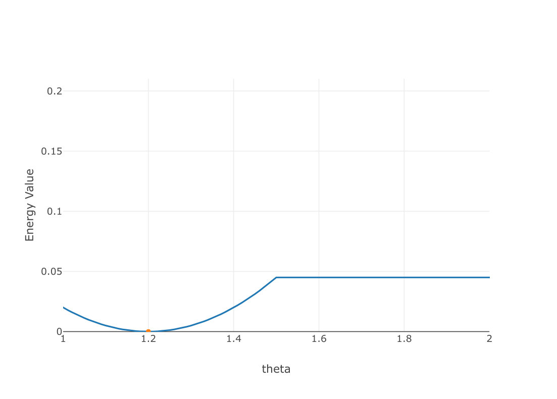 Figure 1
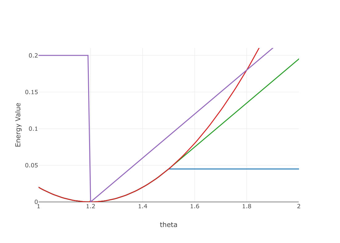 Figure 2
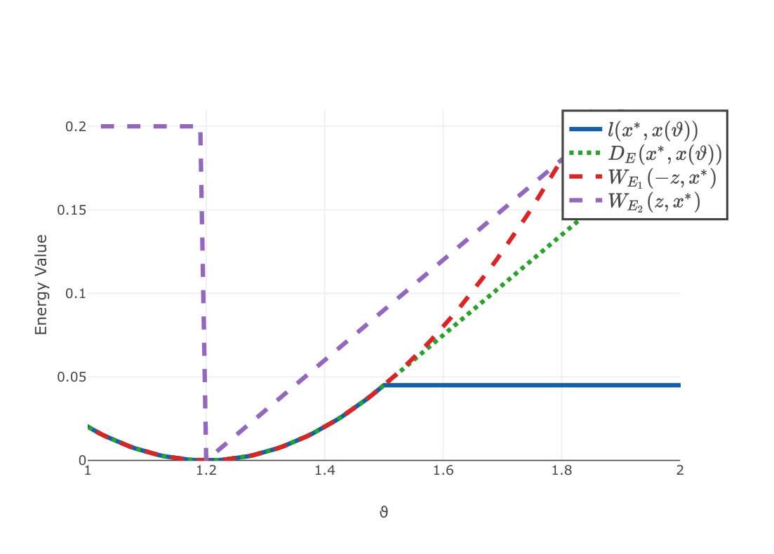 Figure 3
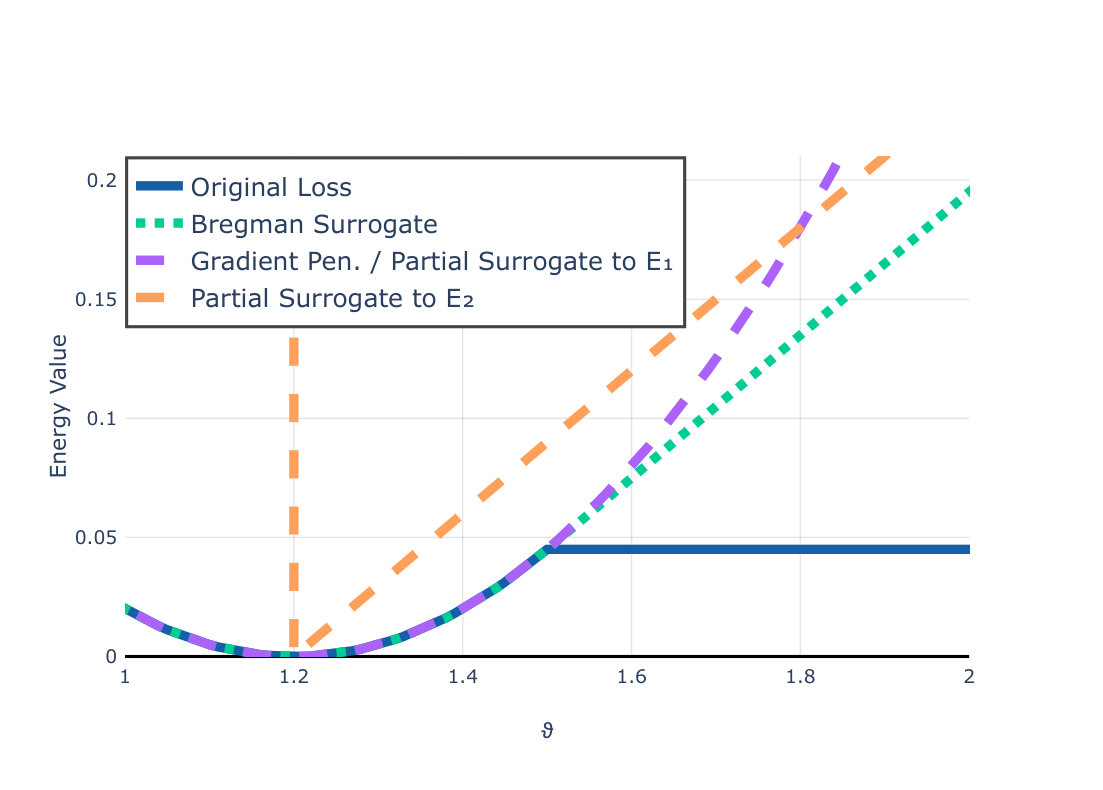 Figure 4
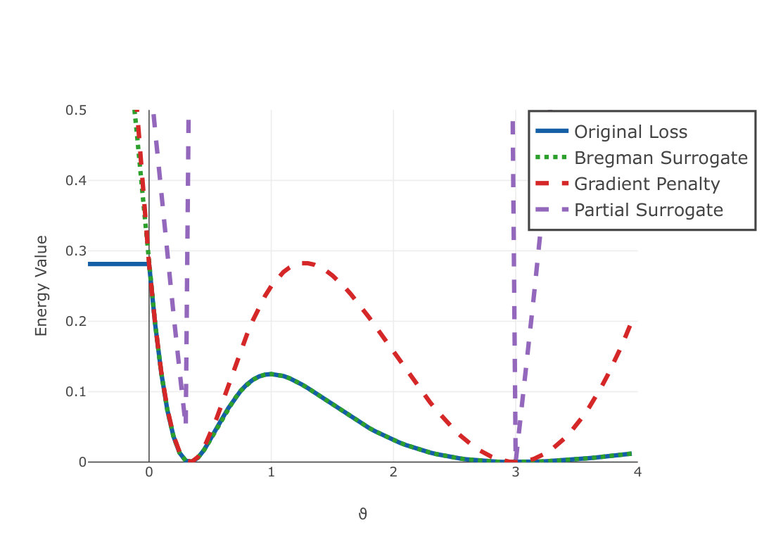 Figure 5
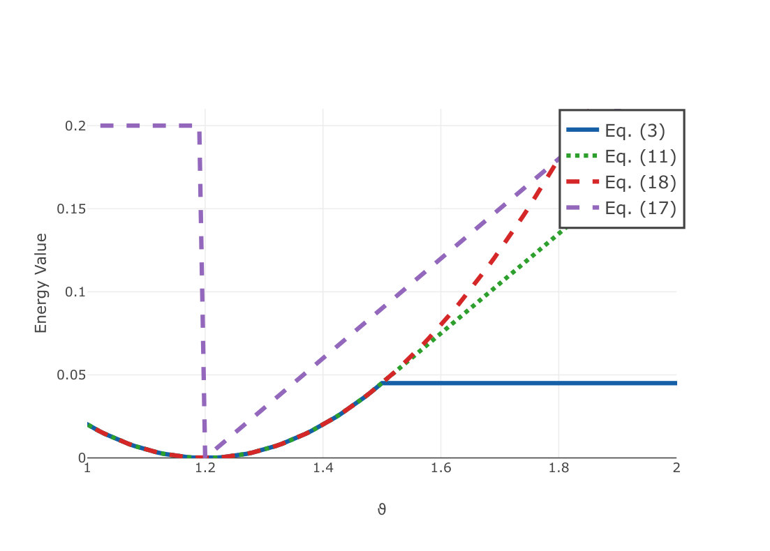 Figure 6
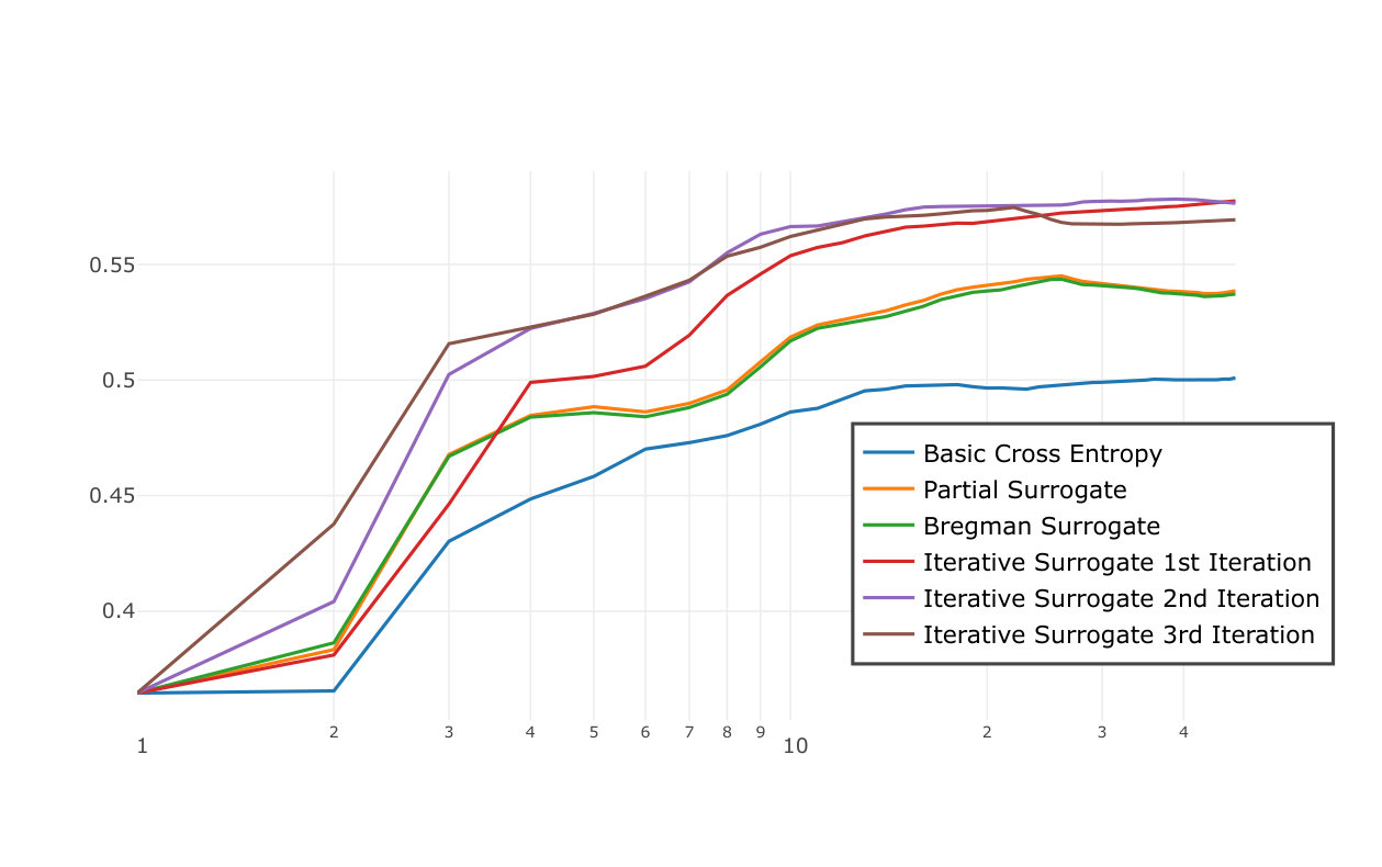 Figure 7
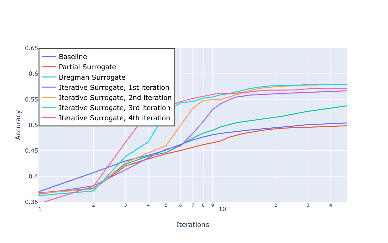 Figure 8
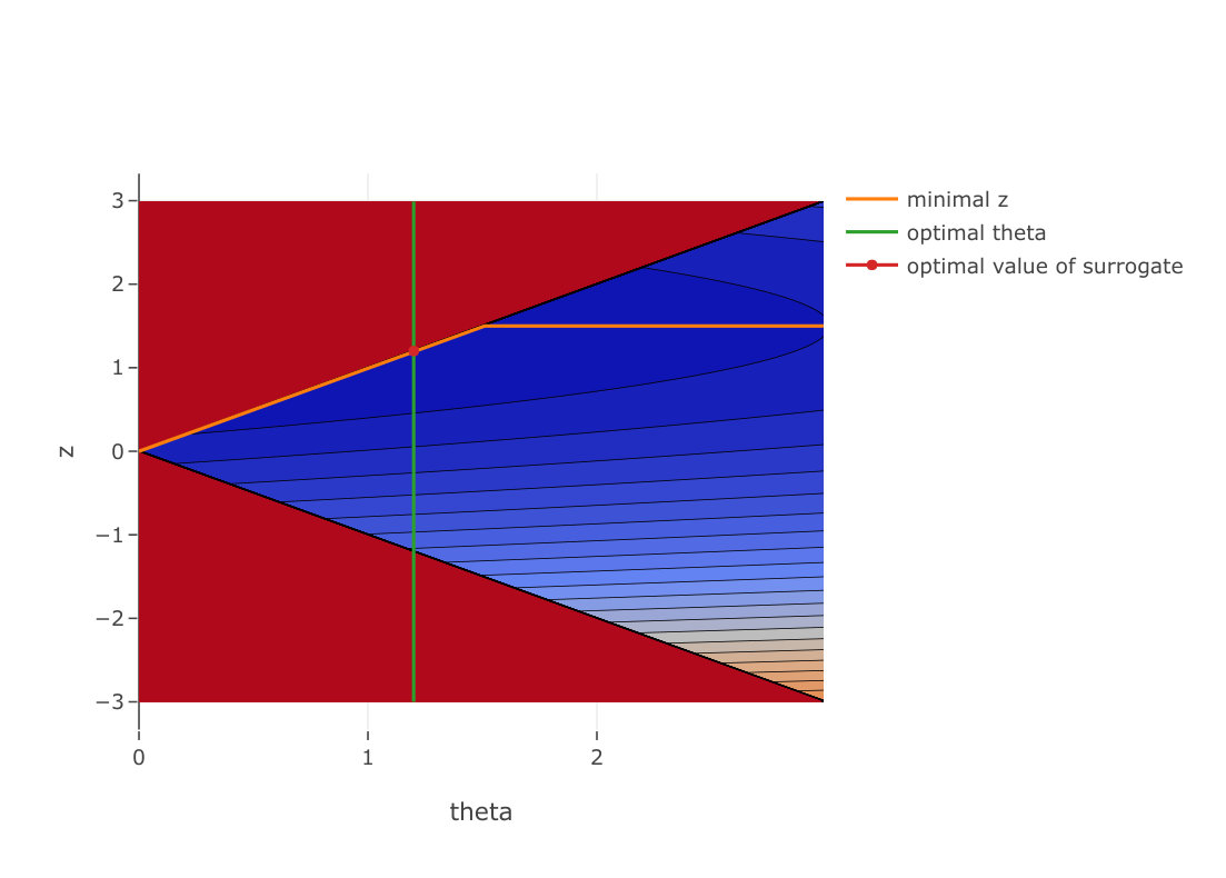 Figure 9
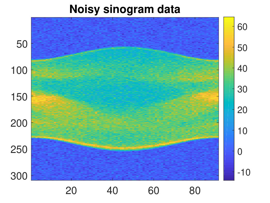 Figure 10
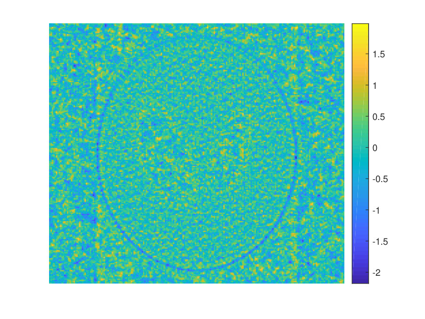 Figure 11
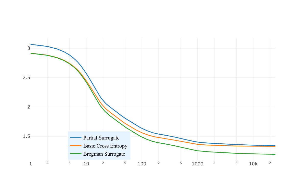 Figure 12
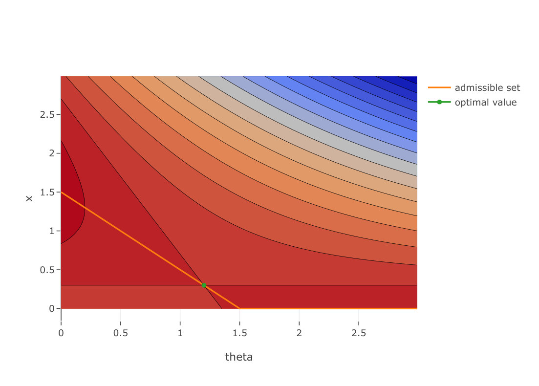 Figure 13
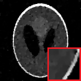 Figure 14
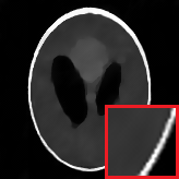 Figure 15
| Model | PSNR | T | PSNR(Iter.) | TT |
|---|---|---|---|---|
| Total Variation | 27.41 | - | - | - |
| 3 3x3 Filters | 26.66 | 00:34 | 27.66 | 02:21 |
| 48 7x7 Filters | 27.41 | 02:45 | 28.03 | 03:11 |
| 96 9x9 Filters | 27.46 | 01:43 | 28.03 | 02:22 |
Peer Reviews
No public reviews on file for this paper yet. If you reviewed it on a platform where reviews are public (OpenReview, ICLR, NeurIPS, ICML), you can paste yours below so the community can read it here.
Code & Models
Videos
No videos yet. Explain this paper in a talk, walkthrough, or lecture? Add one.
Parametric Majorization for Data-Driven Energy Minimization Methods
Jonas Geiping Michael Moeller
Department of Electrical Engineering and Computer Science, University of Siegen
{jonas.geiping, michael.moeller}@uni-siegen.de
Abstract
Energy minimization methods are a classical tool in a multitude of computer vision applications. While they are interpretable and well-studied, their regularity assumptions are difficult to design by hand. Deep learning techniques on the other hand are purely data-driven, often provide excellent results, but are very difficult to constrain to predefined physical or safety-critical models. A possible combination between the two approaches is to design a parametric energy and train the free parameters in such a way that minimizers of the energy correspond to desired solution on a set of training examples. Unfortunately, such formulations typically lead to bi-level optimization problems, on which common optimization algorithms are difficult to scale to modern requirements in data processing and efficiency. In this work, we present a new strategy to optimize these bi-level problems. We investigate surrogate single-level problems that majorize the target problems and can be implemented with existing tools, leading to efficient algorithms without collapse of the energy function. This framework of strategies enables new avenues to the training of parameterized energy minimization models from large data.
1 Introduction
Energy minimization methods, also referred to as variational methods, are a classical tool in computer vision [83, 18, 32, 14]. The idea is to define a data-dependent cost function that assigns a value to each candidate solution . The desired optimal solution is then the target solution with the lowest energy value. This methodology has several advantages, for one, it is characterized by an explicit model - namely the energy function to be minimized - and an implicit inference method - how we compute the minimizer of this energy is a separate problem. This duality allows a fruitful analysis, leading to controllable methods with provable guarantees that are paramount in many critical applications [80, 78, 98]. Furthermore, explicit knowledge over the model structure allows for explainable and clear modifications when the method is applied in a related task [26].
Conversely, deep learning approaches [60], specifically deep feed-forward neural networks work by very different principles. The methodology of deep learning is characterized by implicit models and explicit inference. The solution to the problem at hand is given directly by the output of the learned feed-forward structure. This is advantageous in practice and crucial for the efficient training of neural networks, however the underlying model of the problem structure is now only implicitly contained in the responses of the network. Deep neural networks have fundamentally changed the state-of-the-art in various computer vision applications, due to these properties as the inference operations are learned directly from large amounts of training data. These approaches are able to learn expressive and convincing mechanisms, examples of which can be found not only in recognition tasks (e.g. [56]), but also in denoising [99], optical flow [70, 49] or segmentation tasks [64, 81, 21]. Yet, as the underlying model is only implicitly defined and ’hidden’ in the network structure, it is difficult to modify it for applications in other domains or to guarantee specific outputs. Domain adaptation is still an active field of research and several examples, for instance in medical imaging [3, 38], have demonstrated the need for possibly model-based physically plausible output restrictions. This problem is most strikingly demonstrated by the phenomenon of adversarial examples [89] - the existence of input data, that, when fed through the network, leads to highly erroneous solutions. While one would expect that such behaviour is possibly unavoidable in recognition tasks [87, 71], it should not be a factor in low-level computer vision applications.
Reviewing these two methodologies, we would - of course - prefer to have the best of both worlds. We would like to use both the large amounts of data at our disposal and our far-reaching domain knowledge in many tasks to train explicit models with a significant number of free parameters, so that their optimal solutions are similar to directly trained feed-forward networks.
A promising candidate for such a combination of learning- and model based approaches are parametrized energy minimization methods. The idea of such methods is to define an energy that depends on the candidate solutions , the input data and parameters ,
[TABLE]
such that for a good choice of parameters , the argument that minimizes the energy over all is as close a possible to the desired true solution .
To train such parametric energies, assume we are given training samples and a continuous higher-level loss function , which measures the deviation of solutions of the model to the given training samples. Determining the optimal parameters then becomes a bi-level optimization problem combining both the higher-level loss function and the lower-level energy,
[TABLE]
Usual first-order learning methods are difficult to apply in this setting. For every gradient computation it is necessary to compute a derivative of the operation of the lower-level problem, which is even further complicated if we consider parametrized non-smooth energy models which are wide-spread in computer vision [32, 14].
Therefore, the goal of this paper is to analyze bi-level optimization problems and identify strategies that allow for efficient approximate solutions. We investigate single-level minimization problems with simple constraints without second-order differentiation, which are applicable even to non-smooth energies. Such forms allow scaling the previously limited training of energy minimization methods in computer vision to larger datasets and increase the effectiveness in applications where it is critical that the solution follows a specific model structure.
In the remainder of this paper we analyze the bi-level optimization problem to develop a rigorous understanding of sufficient conditions for a single-level surrogate strategy for continuous loss functions and convex, non-smooth lower-level energies to be successful. We introduce the concept of a parametric majorization function, show relations to structured support vector machines and provide several levels of parametric majorization functions with varying levels of exactness and computational effort. We extend our approximations to an iterative scheme, allowing for repeated evaluations of the approximation, before illustrating the proposed strategies in computer vision applications.
2 Related Work
The straightforward way of optimizing bi-level problems is to consider direct descent methods [55, 85, 30]. These methods directly differentiate the higher-level loss function with respect to the minimizing argument and descend in the direction of this gradient. An incomplete list of examples in image processing is [13, 26, 24, 25, 33, 34, 41, 45, 46]. This strategy requires both the higher- and lower-level problems to be smooth and the minimizing map to be invertible. This is usually facilitated by implicit differentiation, as discussed in [84, 57, 25, 26]. In more generality, the problem of directly minimizing without assuming that smoothness in leads to optimization problems with equilibrium constraints (MPECs), see [9] for a discussion in terms of machine learning or [36, 35, 37] and [30]. This approach also applies to the optimization layers of [2], which lend themselves well to a reformulation as a bi-level optimization problem.
Unrolling is a prominent strategy in applied bi-level optimization across fields, i.e. MRF literature [4, 69] in deep learning [100, 22, 19, 63] and in variational settings [73, 59, 58, 43, 44, 77]. The problem is transformed into a single level problem by choosing an optimization algorithm that produces an approximate solution to the lower level problem after a fixed number of iterations. is then replaced by . Automatic differentiation [42] allows for an efficient evaluation of the gradient of the upper-level loss w.r.t to this reduced objective
[TABLE]
In general these strategies are very successful in practice, because they combine the model and its optimization method into a single feed-forward process, where the model is again only implicitly present. Later works [27, 23, 43, 44] allow the lower-level parameters to change in between the fixed number of iterations, leading to structures that model differential equations and stray further from underlying modelling. As pointed out in [53], these strategies are more aptly considered as a set of nested quadratic lower-level problems.
Several techniques have been developed in the field of structured support vector machines (SSVMs) [92, 28, 1, 95] that are very relevant to the task of learning energy models, as SSVMs can be understood as bi-level problems with a lower-level energy that is linear in and often a non-continuous higher-level loss. Various strategies such as margin rescaling [92], slack rescaling [95, 97], softmax-margins [40] exist and have also been applied recently in the training of computer vision models in [54, 29], we will later return to their connection to the investigated strategies.
3 Bi-Level Learning
We now formalize our learning problem. We assume the lower-level energy from (1) to be convex (but not necessarily smooth) in its first variable and to depend continuously on input data and parameters . We assume its minimizer to be unique. For our higher-level loss function (2) , we assume that it fulfills for all and is differentiable in its second argument.
Note that this formulation of bi-level optimization problems directly generalizes classical supervised (deep) learning with a network via the quadratic energy , for which .
Preliminaries (Convex Analysis): Let us summarize our notation and some fundamental results from convex analysis. We refer the reader to [6] for more details. We denote by the set of subgradients of a convex function at . We define the Bregman distance between two vectors relative to a convex function by for a subgradient , intuitively the Bregman distance measures the difference of the energy at to its linear lower bound around . is the convex conjugate of . is a minimizer of the energy if and only if or equivalently by convex duality . is -strongly convex if for all . Conversely, if is -strongly convex, then is -strongly smooth, i.e. . Furthermore holds for all Bregman distances [11]. We consider parametrized energies in several variables, yet we always assume (sub)-gradients, Bregman distances and convex conjugates to be with respect to the first argument .
3.1 Majorization of Bi-level Problems
As previously discussed, directly solving the bi-level problem as posed in Eq. (2) and (3) is tricky. We need to implicitly differentiate the minimizing argument for all samples just to apply a first-order method in - which is in stark contrast to our goal of finding efficient and scalable algorithms.
Let us instead look at the problem from a very different angle and entertain the idea that the loss function is actually of secondary importance to us. We really only want to find parameters so that our training samples are well reconstructed, . If we go so far as to assume that the loss value of our optimal parameters is zero, meaning that minimizers of our energy are perfectly able to reconstruct our training samples, then the bi-level problem is reduced to a single-level problem, inserting :
[TABLE]
which we could solve via
[TABLE]
This train of thought is closely interconnected to the notion of separability in Support Vector Machine methods [96], where it is assumed that given training samples are linearly separable, which is equivalent to assuming that the classification loss is zero on the training set.
However minimizing Eq. (6) is often not a good choice. A simple example is , i.e. we simply try to learn a positive scaling factor between and . Problem (5) can then be written as and is trivially minimized by . Such a solution makes independent of such that every becomes a minimizer. This phenomenon is referred to as collapse of the energy function [62, 61] in machine learning literature, and clearly cannot be a good strategy to learn a scaling factor.
Interestingly, the scaling problem can be reformulated into a reasonable (non-collapsing) problem, if we require (6) to majorize the bilevel problem: If we consider the higher-level loss function , then our surrogate problem is clearly not a majorizer for arbitrary . However, if we consider a reformulation of the energy to , then this reformulation leads to a majorizing surrogate . Minimizing now leads to learning the desired scaling factor.
Our toy example motivates us to formalize the concept of majorizing surrogates:
Definition 1** (Parametrized Majorizer).**
Given a bi-level optimization problem in the higher level loss and lower-level energy , we call the function a parametrized majorizer, if
[TABLE]
hold for any .
This definition allows us to formalize our objective further. We investigate replacing the bi-level optimization problem (2), (3) by the minimization of a suitable parametrized majorizer, i.e.
[TABLE]
An immediate conclusion of Definition 1 is that the function now certifies our progress as implies . Moreover, our goal is to choose majorizers in such a way that they yield single-level problems (7), meaning it is not necessary to differentiate an operation to minimize them or to solve an equally difficult reformulation, making them significantly easier to solve.
3.2 Single-Level Majorizers
One possible way to find a majorizer that satisfies the previously postulated properties is by considering the majorizer naturally induced through the Bregman distance of the lower level energy. We assume the following condition
[TABLE]
and propose the surrogate problem
[TABLE]
Condition (8) is an assumption on both the loss function and the energy. It thus delineates the class of bi-level problems that can be attacked with this majorization strategy. However this condition is quite general. For a large class of loss functions, we only need the energy to contain a term that also induces the loss function, a property also known as (relative) strong convexity [94, 65]:
Proposition 1**.**
If the loss function is a Bregman distance induced by a strictly convex function , i.e. , then assumption (8) is fulfilled if the energy is -strongly convex, i.e. if is still a convex function.
Proof: We write as and apply the additive separability of Bregman distances to find , which is greater than or equal to , as is non-negative due to the convexity of . For the usual euclidean loss, this property reduces to strong convexity:
Example 1**.**
If the loss function is given by a squared Euclidean loss, and the energy is -strongly convex, then assumption (8) is fulfilled for the energy .
The question remains whether the proposed surrogate problem (9) is efficiently solvable. We especially wanted to circumvent the differentiation of . However is much easier to solve, in comparison to the original bi-level problem, as we can see in both its primal and its dual formulation. First, from a primal viewpoint, we have
[TABLE]
for some subgradient which we have not specified yet. But, as as is by definition a solution to the lower-level problem, we may take and simplify to
[TABLE]
Now is contained solely in and we can write
Bregman Surrogate:
(10)
This surrogate function is already much simpler than the original bi-level problem. We can minimize (10) either by alternating minimization in and maximization in or by jointly optimizing both variables. However, the problem is still set up as a saddle-point problem which is not ideal for optimization.
Remark*.*
Interestingly, this discriminative formulation is not wholly unfamiliar. We can understand this as an appropriate generalization of generalized perceptron training [62, 61, 90] as discussed as far back as [82]. See the appendix for further details. In vein of this comparison, conditions 1 and 2 from e.g. [62], i.e. conditions on the existence of a margin between the optimal solution and other candidate solutions central to (S)SVM methods [96, 91, 93] are reflected in Proposition 1 in the convex continuous setting. Due to continuity of the energy and loss function we cannot obey a fixed margin, yet we impose that the energy grows at least as fast as the loss function, when we move away from the optimal solution.
We can resolve the saddle-point question by analyzing the surrogate (9) from a dual standpoint, as by Bregman duality [10]
[TABLE]
for . Contrasting this formulation with our initial goal of penalizing the subgradient as in Eq. (6), we see that the Bregman distance induced by is the natural ’distance’ by which to penalize the subgradient in the sense that penalizing the subgradient at with this generalized distance recovers a majorizing surrogate.
We can further simplify the dual formulation by applying Fenchel’s theorem:
[TABLE]
Computing is exactly as difficult as minimizing (as ), so we need to rewrite this surrogate in a tractable manner. To do so, we assume that can be additively decomposed into two parts,
[TABLE]
where both and are convex in their first argument and their convex conjugates are simple to compute. Exploiting that yields
[TABLE]
In comparison to the primal formulation in Eq (10), we have now reformulated the problem from a saddle point problem (minimizing in and maximizing in ) to a pure minimization problem, which is easier to handle. This is a generalization of the dual formulation discussed in the linear context of SSVMs for example in [91, 93].
However for both variants we still need to handle an auxiliary variable. We can trade some of this computational effort for a weaker majorizer by making specific choices for in Eq. (14). To illuminate these choices we introduce the function [76, 12], which allows us to write
[TABLE]
Note that if . As such choosing either or allows us to simplify the problem further. This is especially attractive if is differentiable, as then both surrogates can be computed without auxiliary variables. We will denote these as partial surrogates, owing to the fact that we minimize only one term in (15)
Partial Surrogate:
(16)
Effectively, this reduces the requirements of (14), as only the convex conjugate of needs to be computed. By symmetry, the other partial surrogate follows analogously.
We can finally also return to the previously discussed gradient penalty (6). If our energy is -strongly convex, then its convex conjugate is strongly smooth and we can bound the dual formulation (11) via
Gradient Penalty
(17)
While this formulation allows us to minimize an upper bound on the bi-level problem without either auxiliary variables or knowledge about or , it also is the crudest over-approximation among the considered surrogates as the following proposition illustrates.
Proposition 2** (Ordering of parametric majorizers).**
Assuming the condition from Eq. (8), we find that the presented parametric majorizers can be ordered in the following way:
[TABLE]
The Bregman surrogate (10) majorizes the original loss function and is in turn majorized by the partial surrogate (16) which is majorized by the gradient penalty (17) under the assumption of strong convexity.
Proof.
See appendix. ∎
As a clarifying example, we can simplify these majorizers in the differentiable setting:
Example 2** (Differentiable Energy).**
Let be differentiable and -strongly convex, then the majorizers in Prop. 2 are given by
[TABLE]
3.3 Intermission: One-Dimensional Example
Let us illustrate our discussion with a toy example. We consider the non-smooth bi-level problem of learning the optimal sparsity parameter in the bi-level problem:
[TABLE]
As the lower-level energy is 1-strongly convex and the upper level loss is quadratic holds. Detailed derivations of all three surrogate functions of this example can be found in the appendix. Figure 1 visualizes these surrogates, plotting their energy values relative to . Due to the low dimensionality of the problem, all surrogate functions coincide with the original loss function at the optimal value of . It is further interesting to note that the Bregman surrogate is exactly identical with the original loss function in the vicinity of the optimal value, due to the low dimensionality of the example.
3.4 Iterative Majorizers
We used subsection 3.2 to construct a series of upper bounds to facilitate a trade-off between efficiency and exactness. However what happens if we are not satisfied with the exactness of the Bregman surrogate (9)? This setting can happen especially if and are significantly incompatible and subsequently is large, even for optimal . For example if we try to optimize only a few hyper-parameters we might not at all expect to be close to . This discussion can again be linked to the notion of ’separability’ in SVM approaches [96]: The quality of the majorizing strategy is directly related to the level of ’separability’ of the bi-level problem.
However, we can use the previously introduced majorizers iteratively. To do so we need to develop a majorizer that depends on a given estimate .
Proposition 3**.**
Under the standing assumption that (8) and if the loss function is induced by a strictly convex function , i.e. , we have the following inequality:
[TABLE]
Proof.
It holds that which is equivalent to by the Bregman 3-Point inequality [20, 94]. Using the standing assumption and that we find the proposed inequality. ∎
Assume we are given an estimated solution , then we can use this estimate to rewrite our bound to
[TABLE]
This is a linearized variant of the parametric majorization bound and as such a nonconvex composite majorizer in the sense of [39], as such a key property of majorization-minimization techniques remains in the parametrized setting, choosing :
Proposition 4** (Descent Lemma).**
*The iterative procedure given by repeatedly minimizing the right-hand side of Eq. (21) in and setting is guaranteed to be stable, i.e. not to increase the bi-level loss: *
[TABLE]
Proof.
See appendix. ∎
However this algorithm cannot be applied directly, as we would still need to differentiate appearing in the linearized part. Nevertheless, we can use both Fenchel’s inequality and the previously established to find an over-approximation to the iterative majorizer of Prop. 4:
[TABLE]
This estimate reveals that we can approximate the iterative majorizer much like the previously discussed surrogates:
Iterative Surrogate
(22)
as the constant does not depend on . We essentially return to Eq. (12) and only the input to and changes with respect to . This strategy recovers the previous majorizer as a special case:
Corollary 1**.**
If we linearize around , then we recover the Bregman surrogate of (9).
Proof.
If , then and by the properties of the differentiable loss function. As such the constant term is zero and so that we recover (12) which is equivalent to the Bregman surrogate (9). ∎
We can use this surrogate to form an efficient approximation to a classical majorization-minimization strategy as in [88, 67, 66, 48]. Notably the ’tightness’ of the majorization is violated by the over-approximation, i.e. inserting into the majorizer does not recover . We iterate
[TABLE]
As the application of this iterative scheme reduces to a simple change from Eq (12) to Eq. (22), we can easily apply it in practice to further increase the fidelity of the surrogate by solving a sequence of fast surrogate optimizations. We initialize the scheme with as suggested from Corollary 1 and either stop iterating or reduce the step size of the surrogate solver if the higher-level objective is increased after an iteration.
4 Examples
This section will feature several experiments111An implementation of these experiments can be found at https://github.com/JonasGeiping/ParametricMajorization. in which we will illustrate the application of the investigated methods. We will show two concepts of new applications that are possible in parametrized variational settings, 4.1 and 4.2. We then show an application to image denoising in 4.3.
4.1 Computed Tomography
Making only specific parts of a variational model learnable is especially interesting for computed tomography (CT). An image is to be reconstructed from data that is formed by applying the radon transform to the image and adding noise . While first fully-learning based solutions to this problem exist (e.g. [50, 51]), suitable networks are difficult to find not only due to the ill-posedness of the underlying problem, but also due to the well-justified concerns about fully learning-based approaches in medical imaging [3]. To benefit from the explicit control of the data fidelity of the reconstruction, we consider to introduce a learnable linear correction term into an otherwise classical reconstruction technique via
[TABLE]
for a suitable network (we chose 8 blocks of convolutions with 32 filters, ReLU activations, and batch-normalization, and a final convolution), and denoting the Huber loss of the discrete gradient of .
As both convex conjugates are difficult to evaluate in closed-form, we choose the gradient penalty (17), which is a parametric majorizer for euclidean loss if has full rank (and practically even works beyond this setting, as it majorizes even for rank-deficient ). According to (17) we consider
[TABLE]
train on simulated noisy data and test our model on the widely-used Shepp-Logan phantom. Figure 2 illustrates the the resulting reconstruction, as well as the best reconstruction using the variational approach without the additional linear correction term after a grid-search for the optimal . As we can see, the surrogate trained the linear correction term well enough to improve the PSNR of the reconstruction by almost 2dB. Moreover, the influence of the linear correction term can still be visualized and the data fidelity can easily be controlled via a suitable weighting. We visualize the correction map in the appendix.
4.2 Variational Segmentation
For a very different (and non-smooth) example, consider the task of learning a variational segmentation model [18, 15, 32, 72]. We are interested in learning a model whose minimizer coincides with a (semantic) segmentation of the input data. The lower-level problem is given by
[TABLE]
where is the entropy function on the unit simplex [7]. is some parametrized function that computes the potential of the segmentation model, this can be a deep neural network, as we only require convexity in and not in . is a finite-differences operator, so that the overall total variation (TV) term measures the perimeter of a segmentation if . The entropy function crucially not only leads to a strictly convex model but also represents the structure of a usual learned segmentation method. Without the perimeter term, a solution to the lower-level problem would be given by
[TABLE]
Due to [79, P.148], is exactly the function, so that Eq. (25) is equivalent to applying a parametrized function and then applying the function to arrive at the final output, a usual image recognition pipeline during training. As a higher-level loss, we choose loss
[TABLE]
so that the bi-level problem without the perimeter term is equivalent to minimizing the cross-entropy loss of . With the inclusion of the perimeter term, however, we cannot find a closed-form solution for need to consider bi-level optimization.
But, as the log-loss (26) can be written as a Bregman distance relative to , our primary assumption (8) is fulfilled and we can consider the Bregman surrogate problem in the dual setting of Eq. (14):
[TABLE]
which we can rewrite to
[TABLE]
We note that this is essentially a cross-entropy loss with an additional additive term , that is able to balance out incoherent output of that would lead to erroneous segmentations with a higher perimeter. Furthermore, the training process is still convex w.r.t to , in contrast to unrolling schemes. The iterative model (23) has a very similar structure, including the gradient of the loss into (28).
To validate this setup, we choose to be given by a simple convolutional linear model. We draw a small subset of the cityscapes dataset and compare the cross entropy model of Eq (25) with the total variation bi-level model of Eq. (28) and its partial and iterative applications. Figure 3 visualizes the training accuracy over training iterations. We find that the proposed approach is able to improve the segmentation accuracy of the linear model significantly. We refer to the appendix for further details.
4.3 Analysis Operator Models
Finally, we illustrate the behaviour of our approach on a practically relevant model, learning a set of optimal convolutional filters for denoising [83, 26]. We consider the parametric energy model
[TABLE]
with denoting the convolution operator to be learned, which is prototypical for many other image processing tasks. We consider square loss as a higher loss function and apply our approach. A Bregman surrogate for this model has the form
[TABLE]
Model (29) was previously considered in [26, 24], where it was solved via implicit differentiation. We repeat the setup of [26] and train a denoising model on the BSDS dataset [68]. Refer to the appendix for the experimental setup and optimization strategy.
Table 1 shows both PSNR values achieved when training as convolutional filters as well as training time. In comparison to [26], we find strikingly, that we can train a convex model with similar performance to the convex model in [26], while being an order of magnitude faster than the original approach. Furthermore in [26], the necessary training time jumps from 24 hours for 48 7x7 filters to 20 days for 96 9x9 filters - in our experiment the training time is almost unaffected by the number of parameters, and in this example actually smaller as the larger model converges faster. Also this analysis validates that the iterative process is crucial to reaching competitive PSNR values.
5 Conclusions
We investigated approximate training strategies for data-driven energy minimization methods by introducing parametric majorizers. We systematically studied such strategies in the framework of convex analysis, and proposed the Bregman distance induced by the lower level energy as well as over-approximations thereof as suitable majorizers. We discussed an iterative scheme that shows promise for applications in computer vision, particularly due to its scalability as shown by its application to image denoising.
Appendix A Appendix
A.1 Convex Analysis in Section 3
A.1.1 Details for Derivation of Eqs. (11), (12)
Eq. (11) above describes the application of Bregman duality:
[TABLE]
which is a common application of the following identity [11, 10]:
Lemma 1** (Bregman Identity).**
Consider a convex lsc. function with a subgradient . Then, the following identity holds:
[TABLE]
Proof.
This property follows from equality (Fenchel’s identity) in the Fenchel-Young inequality . To see this we write
[TABLE]
and apply Fenchel’s identity for to find
[TABLE]
We then introduce any by writing and apply Fenchel’s identity again:
[TABLE]
∎
The step from Eq. (11) to Eq.(12) is simply the first step of this derivation:
[TABLE]
as is a subgradient of at and at .
A.1.2 Details for Derivation of Eq. (14) to (15)
A crucial subtlety of Lemma 1 is that this identity holds for any and the choice of subgradients is irrelevant, the Bregman distance is equal for all choices. This motivates the introduction of the -function . This function is convex in either or and always non-negative. It can be understood as measuring the deviation of from subgradients of as a direct implementation of the Fenchel-Young inequality. As such it is 0 exactly if . Previous usage of this function can be found for example in [12, 76]. For Legendre functions [5], i.e. functions where both and are (essentially) smooth, the connection to Bregman distances is immediate:
[TABLE]
for non-smooth functions this is also a part of the proof of Lemma 1, replacing by . As such, we can write Eq. (12) as
[TABLE]
The introduction of this function then allows us to show that
[TABLE]
under the assumption in Eq.(13), that can be written as , with both functions convex. We recognize this as the clear extension of the infimal convolution property (which itself can be understood as Fenchel’s duality theorem applied to , ) to these functions, in the smooth setting this could be written via
[TABLE]
We arrive at Eq. (15) from Eq. (14) by rewriting in Eq.(14):
[TABLE]
A.1.3 Proof of Proposition 2
Proposition 2** (Ordering of parametric majorizers).**
Assuming the condition from Eq. (8), we find that the presented parametric majorizers can be ordered in the following way:
[TABLE]
The Bregman surrogate (10) majorizes the original loss function and is in turn majorized by the partial surrogate (16) which is majorized by the gradient penalty (17) under the assumption of - strong convexity of .
Proof.
The first inequality follows directly by the assumption . The second inequality is the application of Bregman Duality discussed in Lemma 1. From Eq.(15) we now see that , can be written as a minimum over . Clearly choosing a non-optimal yields an upper bound to this minimal value. Without loss of generality, we choose so that is equal to zero.
Now we assume that is -strongly convex. We subsume this strong convexity term in again without loss of generality so that is strongly convex. By convex duality [6], this implies that is strongly smooth, i.e. . Following Eq.(12), we write
[TABLE]
under mild assumptions on the additivity of subgradients of and . ∎
A.1.4 Derivation of the surrogate functions for the example in subsection 3.3
Section 3.3 discusses the non-smooth bi-level problem given in Eqs. (18) and (19):
[TABLE]
for both . In this setting, the ’primal’ formulation of the Bregman surrogate is given by
[TABLE]
whereas the ’dual’ formulation is given by
[TABLE]
Note that this problem is convex in as the epigraph constraint is convex. Both (equivalent!) variants are visualized in Figure 4. We see that the saddle-point of the primal formulation and the minimizer of the dual formulation correctly coincide with the optimal .
Moving forward, we set and to compute the two partial surrogates. Firstly leads to
[TABLE]
where we take as in our example. As is a quadratic function, this is also equivalent to the gradient penalty in Eq. (17). The second partial surrogate, can be written as
[TABLE]
Figure 4 here and Figure 1 in the main paper both arise from the data point .
To give some more details on the fact that the Bregman surrogate is exactly identical with the original loss function in the vicinity of the optimal value, note that this is caused by the special structure of the Bregman distance of the absolute value, as decomposes into . This function is equal to the higher-level loss function as soon as the signs of and coincide and as such the majorizer is exact, even if it is much easier to compute.
A.1.5 Proof of Proposition 4
Section 3.4 describes an iterative procedure for repeated application of the majorization strategies discussed in section 3.2. This scheme was based on the result of Proposition 3:
[TABLE]
inserting leads to
[TABLE]
Eq.(20), respectively (20b), lead to a monotone descent of the higher-level loss, as shown in Proposition 4:
Proposition 4** (Descent Lemma).**
The iterative procedure given by
[TABLE]
is guaranteed to be stable, i.e. not to increase the bi-level loss:
[TABLE]
Proof of Proposition 4.
is a minimizer of the iterative scheme. Therefore, evaluating the iteration at leads to a lower value than evaluating at :
[TABLE]
Now the left-hand-side is also equivalent to Eq. (20b) evaluated at . Applying the inequality in (20b) for all we find
[TABLE]
∎
Remark*.*
The iterative scheme given in Eq.(22), i.e.
[TABLE]
is an over-approximation of the iterative scheme discussed in Proposition 4. As such we expect the results of Proposition 4 to hold only approximately as stated in the main paper.
A.2 Experimental Setup
This section will add additional details to the experiments presented in the paper222Refer also to the implementations hosted at https://github.com/JonasGeiping/ParametricMajorization.
A.2.1 CT - Additional Details
The implementation of the CT example in section 4.1 is straightforward. We generate pairs of noisy sinograms and ground truth images and optimize
[TABLE]
We test our model on the widely-used Shepp-Logan phantom, comparing the learned model with a pure Huber-TV solution, for which we found the optimal parameter by grid search. This setup was implemented in Matlab. To visualize the linear correction term, we repeat an extended version of Figure 2 in Figure 5.
A.2.2 Segmentation - Additional Details
The segmentation experiment shown in Figure 3 of the main paper shows the results of training the variational model in Eq.(25), which corresponds to an augmented cross-entropy term, as discussed in section 4.2.
The partial surrogate implemented in Figure 3 is a direct application of Eq.(16) to the segmentation setting, giving
[TABLE]
where the computation of the auxiliary variable is simplified. Note further that the gradient penalty cannot be applied in this setting, as the segmentation energy is not strongly convex. Similarly, the iterative approach can be computed to be
[TABLE]
which is still convex in , but the input arguments now take previous solutions into account.
To emphasize the convexity of the setup, we choose as a linear convolutional network of filters for each target class. We accordingly optimize the resulting convex minimization problems by an optimal convex optimization method, namely FISTA [8]. To solve the inference problem in Eq. (25) we apply usual strategies and optimize via a primal-dual algorithm [16] - to increase the speed we adapt a recent variant [17] and consider the Bregman-Proximal operator in the primal sub-problem for which we use the entropy function described in the paper, paralleling [7, 74].
We draw four images and their corresponding segmentations from the cityscapes data set [31] and implement the proposed procedures in PyTorch [75]. For Figure 3 we drew the first four images, which we resized to 128x256 pixels. To visualize the improvement over the iterations, we initialize the subsequent iterations of the iterative scheme again with the initial value of , so that the training accuracy curves in Figure 3 are comparable. This is of course not strictly necessary and could be initialized with the current estimate in every iteration. We also point out that we visualize the actual training accuracy in Figure 3, meaning the percentage of successfully segmented pixels after hard argmax of the results of the algorithms.
A.2.3 Analysis Operators - Additional Details
For this experiment we considered the task of learning an ’analysis operator’ , i.e. a set of convolutional filters so that for a set of filters. Due to anisotropy, we can write the resulting minimization problem as
[TABLE]
We repeat the experimental setup of [26] and train this model on image pairs of noise-free and noisy image patches, to learn filters that result in a convex denoising model [25, 26]. To do so we draw a batch of 200 image patches from the training set of the Berkeley Segmentation data set [68], convert the images to gray-scale and add Gaussian noise. To compare with [26] and [99] we do not clip the noisy images and use Matlab’s rgb2gray routine to generate this data. Further, as in [26], we do not optimize directly for the convolutional filters, but instead decompose each filter into a DCT-II basis, where we learn the weight of each basis function, excluding the constant basis function [47]. Before training we initialize these weights by orthogonal initialization [86] with a factor of , respectively for the larger 9x9 filters.
To solve the training problem we minimize Eq. (33) in the paper jointly in . We do this efficiently by taking steps toward the optimal weights with the ’Adam’ optimization procedure [52] with a step size (although gradient descent with momentum or FISTA [8] are also valid options). We use a standard accelerated primal-dual algorithm [16] to solve the convex inference problem. For the iterative procedure we repeat this process, computing after every minimization of Eq.(33), inserting it as a factor into and repeating the optimization. If the iterative procedure increases the loss value, we reduce the step size of the majorizing problem and repeat the step. If reducing the step size does not successfully improve the result for several iterations, we terminate the algorithm.
We implement this setup in PyTorch [75] and refer to our reference implementation for further details.
For total variation denoising, which corresponds to choosing as the gradient operator with appropriate scaling, , we use grid search to find the optimal scaling parameter .
We report execution times for a single minimization of Eq.(33) for different filter sizes in Table 1 in the paper as well as total time for an iterative procedure. These timings are reported for a single GeForce RTX 2080Ti graphics card.
The reference list from the paper itself. Each links out to its DOI / PubMed record.
- 1[1] Yasemin Altun, Ioannis Tsochantaridis, and Thomas Hofmann. Hidden Markov Support Vector Machines. In Proceedings of the Twentieth International Conference on International Conference on Machine Learning , ICML’03, pages 3–10. AAAI Press, 2003.
- 2[2] Brandon Amos and J. Zico Kolter. Opt Net: Differentiable Optimization as a Layer in Neural Networks. In International Conference on Machine Learning , pages 136–145, July 2017.
- 3[3] Vegard Antun, Francesco Renna, Clarice Poon, Ben Adcock, and Anders C. Hansen. On instabilities of deep learning in image reconstruction - Does AI come at a cost? ar Xiv:1902.05300 [cs] , Feb. 2019.
- 4[4] Adrian Barbu. Learning real-time MRF inference for image denoising. 2009 IEEE Conference on Computer Vision and Pattern Recognition , pages 1574–1581, 2009.
- 5[5] Heinz H Bauschke and Jonathan (Jon Borwein. Legendre Functions and the Method of Random Bregman Projections. Journal of Convex Analysis , 4(1):27–67, May 1997.
- 6[6] Heinz H. Bauschke and Patrick L. Combettes. Convex Analysis and Monotone Operator Theory in Hilbert Spaces . CMS Books in Mathematics. Springer New York, New York, NY, 2011.
- 7[7] Amir Beck and Marc Teboulle. Mirror descent and nonlinear projected subgradient methods for convex optimization. Operations Research Letters , 31(3):167–175, May 2003.
- 8[8] Amir Beck and Marc Teboulle. A Fast Iterative Shrinkage-Thresholding Algorithm for Linear Inverse Problems. SIAM Journal on Imaging Sciences , 2(1):183–202, Jan. 2009.
