QCD Axion on Hilltop by a Phase Shift of $\pi$
Fuminobu Takahashi, Wen Yin

TL;DR
This paper proposes a novel mechanism called "πnflation" where a heavy axion induces a phase shift of approximately π, setting the QCD axion's initial misalignment angle near π, which can explain dark matter and has testable predictions.
Contribution
The paper introduces the πnflation mechanism involving a heavy axion to set the initial axion angle near π, linking it to hilltop inflation and observable signals.
Findings
QCD axion with f_a ≥ 3×10^9 GeV can account for dark matter via πnflation.
Parameter regions overlap with upcoming experimental sensitivities like ORGAN, MADMAX, TOORAD, and IAXO.
Implications for neutrino species and isocurvature perturbations are discussed.
Abstract
We show that the initial misalignment angle of the QCD axion (or axion-like particles) can be set very close to , if the QCD axion has a mixing with another heavy axion which induces the phase shift after inflation. In the simplest case, the heavy axion plays the role of the inflaton, and we call such inflation as "nflation." The basic idea was first proposed by Daido and the present authors in Ref. [1702.03284] in 2017 and more recently discussed in Ref. [1903.00462]. We show that the QCD axion with a decay constant GeV can explain dark matter by the nflation mechanism. A large fraction of the parameter region has an overlap with the projected sensitivity of ORGAN, MADMAX, TOORAD and IAXO. We also study implications for the effective neutrino species and isocurvature perturbations. The nflation can provide an initial…
Click any figure to enlarge with its caption.
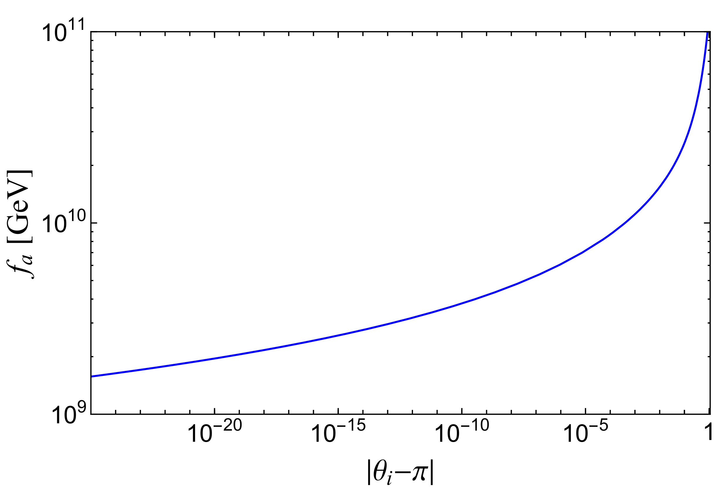 Figure 1
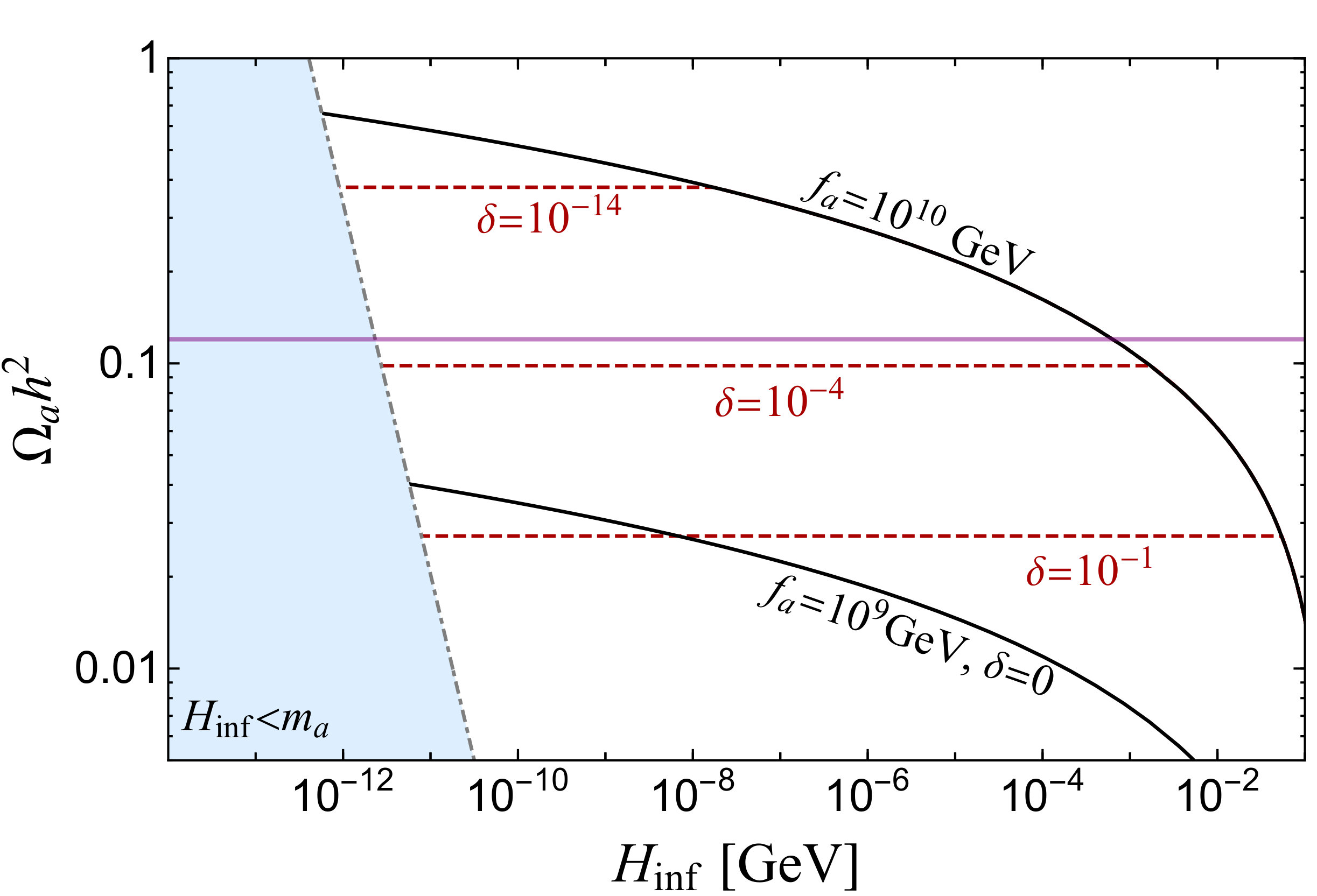 Figure 2
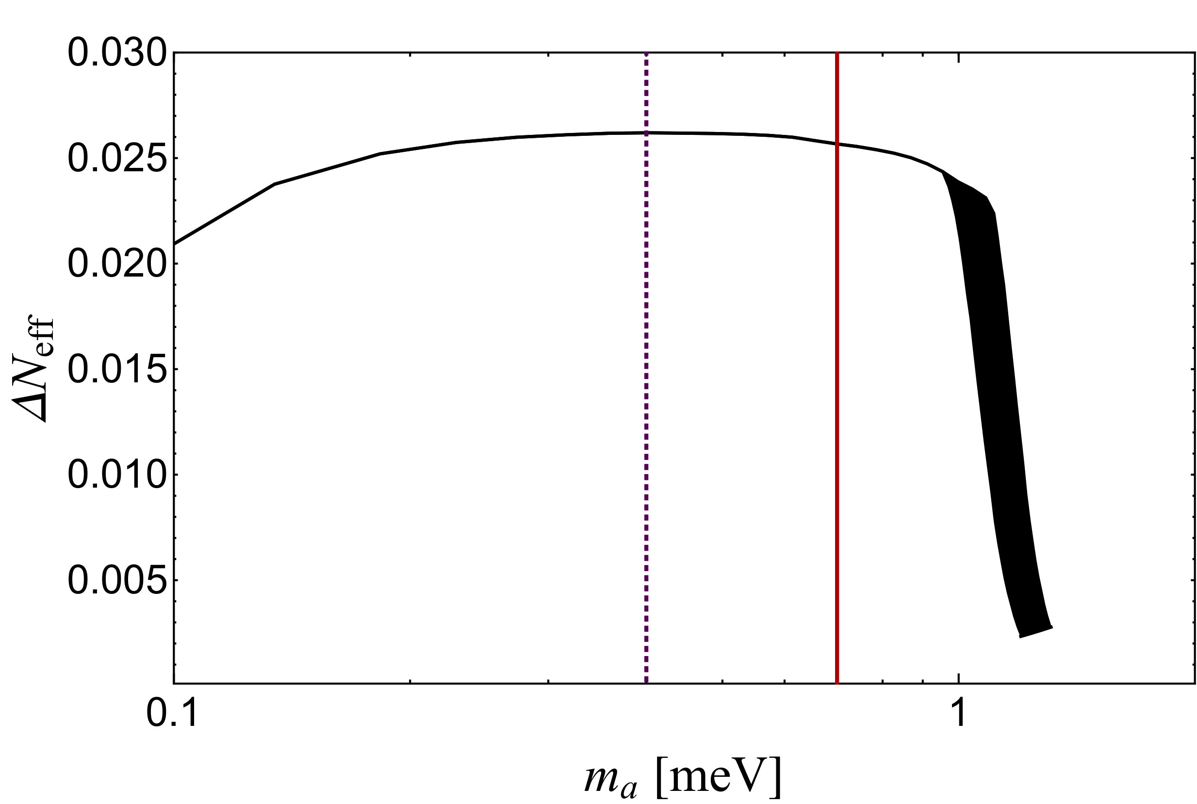 Figure 3
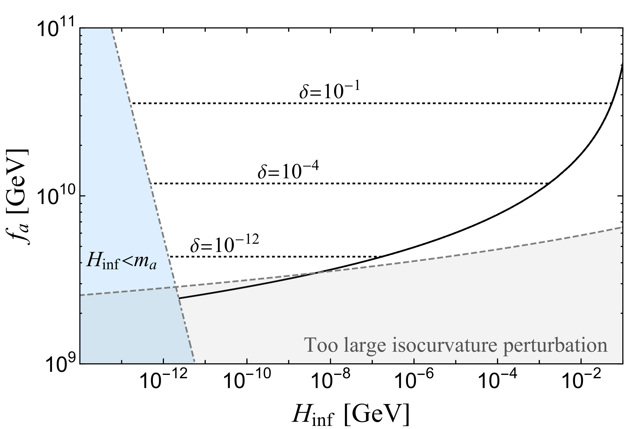 Figure 4
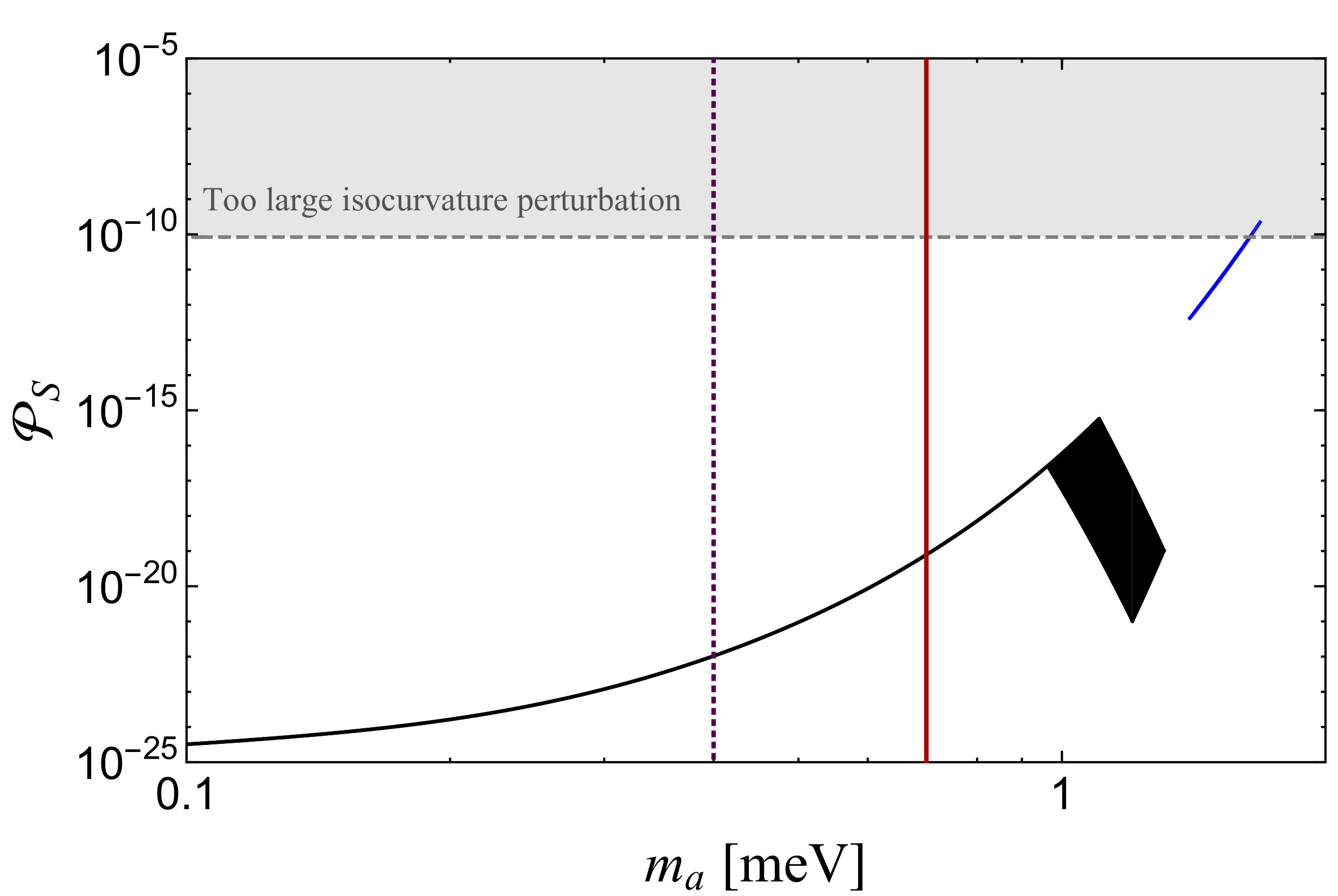 Figure 5
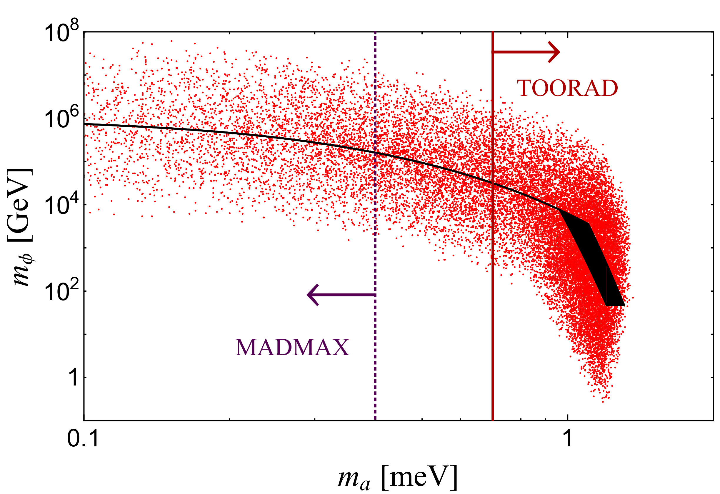 Figure 6
Peer Reviews
No public reviews on file for this paper yet. If you reviewed it on a platform where reviews are public (OpenReview, ICLR, NeurIPS, ICML), you can paste yours below so the community can read it here.
Videos
No videos yet. Explain this paper in a talk, walkthrough, or lecture? Add one.
TU-1091
IPMU19-0112
**QCD Axion on Hilltop by a Phase Shift of
**
Fuminobu Takahashi1,2, Wen Yin3
*1**Department of Physics, Tohoku University, Sendai, Miyagi 980-8578, Japan
2Kavli Institute for the Physics and Mathematics of the Universe (WPI), University of Tokyo, Kashiwa 277–8583, Japan
3 Department of Physics, KAIST, Daejeon 34141, Korea *
Abstract
We show that the initial misalignment angle of the QCD axion (or axion-like particles) can be set very close to , if the QCD axion has a mixing with another heavy axion which induces the phase shift after inflation. In the simplest case, the heavy axion plays the role of the inflaton, and we call such inflation as “nflation.” The basic idea was first proposed by Daido and the present authors in Ref. [1] in 2017 and more recently discussed in Ref. [2]. We show that the QCD axion with a decay constant GeV can explain dark matter by the nflation mechanism. A large fraction of the parameter region has an overlap with the projected sensitivity of ORGAN, MADMAX, TOORAD and IAXO. We also study implications for the effective neutrino species and isocurvature perturbations. The nflation can provide an initial condition for the hilltop inflation in the axion landscape, and in a certain set-up, a chain of the hilltop inflation may take place.
1 Introduction
The QCD axion [3, 4, 5, 6] is a plausible candidate for dark matter (DM). It starts to oscillate about the CP conserving minimum, when its temperature-dependent mass becomes comparable to the Hubble parameter during the QCD phase transition [7, 8, 9]. The abundance of the QCD axion generated by the misalignment mechanism is given by [10, 11, 12]
[TABLE]
where
[TABLE]
is the initial misalignment angle, and is the axion decay constant. The coefficient is given by
[TABLE]
which takes account of the anharmonic effect. Here and in what follows the QCD axion is stabilized at the CP conserving minimum, , in the present vacuum.
One can see from Eq. (1) that the QCD axion explains the observed DM abundance, [13], for and GeV. This sets the upper bound of the so-called classical axion window, GeV. This does not preclude the possibility of larger or smaller values of . Larger is possible if is (much) smaller than unity. This can be realized by fine-tuning based on the anthropic argument [14, 15, 16], or very low-scale inflation [17, 18].111Alternatively, one may modify thermal history of the Universe [9, 19, 20, 21, 22], or introduce the explicit PQ breakig by the Witten effect to suppress the QCD axion abundance [23, 24, 25, 26]. On the other hand, smaller is possible if the initial position of the QCD axion is close to the hilltop of the potential, i.e., . In the hilltop limit, the anharmonic coefficient, , logarithmically increases; e.g. and As a result, the QCD axion abundance can be enhanced if is close to In Fig. 1 we show the relation between and to explain the observed DM abundance.
In the hilltop limit, the power spectrum of the axion isocurvature perturbation [27, 28] as well as its non-Gaussianity [28] are also significantly enhanced.222 Before Ref. [28], there were some inconsistencies among the literature concerning the power spectrum of the axion isocurvature perturbations in the hilltop limit. Therefore, the axion DM with relatively small poses two issues. One is the fine-tuning of the initial misalignment angle near . The other is that one needs very low-scale inflation to satisfy the isocurvature bound.
Smaller implies a heavier QCD axion mass, which is challenging from the experimental point of view. Many experiments for axion DM search have been proposed so far, and some of them are aiming at such relatively heavy axion masses. The range of the axion mass partially overlaps with the mass range expected by the axion production mechanism using the string-wall network [29, 30, 31, 32, 33]. However, there are currently uncertainly in the estimate as one has to rely on a large amount of extrapolation from the parameters used in the numerical calculations to the realistic ones [34].
In this paper we provide a mechanism to set the initial position of the QCD axion very close to the hilltop of the potential. We consider an inflation model where another axion plays the role of the inflaton. Being the axion, the inflaton has a potential with the periodicity , where is the inflaton decay constant. For instance, successful slow-roll inflation is possible if the potential consists of two cosine terms, which is known as the multi-natural inflation [35, 36, 37, 38, 39]333 See Ref. [1, 40, 2] for realization of the multi-natural inflation in terms of an axion-like particle.. The inflation takes place on the flat plateau around the potential maximum, and after inflation ends, the inflaton rolls down toward the nearest potential minimum. The distance between the maximum and the minimum is naturally equal to or very close to multiplied by .444 Depending on the details of the inflaton potential, it can be a fraction of . A more precise explanation will be given later.
We assume that the Hubble parameter during inflation is lower than the QCD scale so that the QCD axion acquires the potential during inflation. Then, if the inflaton has a mixing with the QCD axion555 The mass and kinetic mixings between the QCD axion and another axion were discussed in e.g. Refs. [41, 42, 43, 44, 45], where the level crossing between the two axions can reduce the axion abundance. The mixing can also induce the DM decay [46, 1, 47]. Also the mixing between axions plays an important role in inflation model building [48, 49, 50, 51, 52, 53] , the sign of the QCD axion potential is flipped by the phase shift of due to the inflaton dynamics. The role of the inflation model is twofold. First, the inflation scale is so low that the QCD axion is naturally located near the potential minimum during inflation. The probability distribution of the QCD axion around the potential minimum is determined by the Bunch-Davies (BD) distribution [17, 18]. Second, the inflaton dynamics provides the phase shift of in the axion potential through the mixing, and flips the sign of the potential. In other words, the initial position of the QCD axion is set close to the hilltop. We call such an inflation model that provides the phase shift of as nflation. The nflation resolves the two issues in realizing the QCD axion DM with small simultaneously.
In fact, the basic idea of the nflation was proposed by Daido and the present authors in 2017 [1] where it was shown that the sign of the potential can be flipped by the phase shift close to of the heavy axion via the mass mixing. The main purpose was to explain the initial condition for the hilltop inflation. Recently, we pointed out in Ref. [2] that, if the inflaton has a mixing with the QCD axion, the minimum of the axion potential can be shifted after inflation, inducing coherent oscillations of the QCD axion at a later time when the Hubble parameter becomes comparable to the axion mass. In both cases, the axion mass was assumed to be much smaller than the Hubble parameter during inflation. On the other hand, more recently, Kobayashi and Ubaldi showed in Ref. [47] that the axion that is already stabilized at the potential minimum during inflation can be produced by the inflaton dynamics. The key differences are that they assumed that the axion is heavier than the Hubble parameter during inflation, and they made use of the kinetic mixing instead of the mass mixing.
Recently, Co, Gonzalez, and Harigaya proposed a mechanism that drives the QCD axion to the hilltop of the potential in a supersymmetric framework [54]. The QCD axion has a mass larger than in their set-up due to the enhanced QCD scale [55, 56, 57, 58], and it is stabilized at the potential minimum at that time.666 The axion isocurvature perturbations can be suppressed in this case [58]. See e.g. Refs. [59, 14, 60, 61, 62, 63, 64, 65, 66, 67, 68, 69, 70, 71, 26, 72, 73] for other scenarios to suppress the axion isocurvature.
Their mechanism flips the coefficient of the axion potential. On the other hand, in our scenario, the potential is flipped by the phase shift of by our nflation.
We note that, if the QCD axion is exactly on top of the potential when it starts to oscillate during the QCD phase transition, domain walls will be produced.777 FT thanks Keisuke Harigaya for discussion on this point. Such domain walls without strings are stable and spoil the success of the standard cosmology. The cosmological catastrophe may be avoided if the initial position is slightly deviated from the CP conserving minimum (or maximum). In our scenario, the QCD axion remains light and follows the BD distribution during inflation. Thus, it is naturally deviated from the potential minimum by a small amount which is determined by the inflation scale.
The rest of this paper is organized as follows. In the Sec. 2 we present the basic idea of nflation and show that the QCD axion with GeV can explain DM due to nflation. In Sec. 3 we provide a concrete nflation model and study its experimental and observational implications. The last section is devoted to discussion and conclusions.
2 Basic idea
In this section we explain the basic idea of the nflation and its implications for the QCD axion abundance and isocurvature perturbations.
2.1 nflation
Let us introduce an inflaton field, , and the QCD axion, .888 Our mechanism works even if is not the inflaton, as long as changes its field value by mod after inflation. Both fields enjoy the following discrete shift symmetry,
[TABLE]
where and are the decay constants of and , respectively. This implies that the potential is periodic with respect to both and .
In order not to spoil the Peccei-Quinn mechanism as a solution to the strong CP problem, there must be a flat direction when one turns off the QCD interactions. Then, after a certain field redefinition, the potential can be given by the following form,
[TABLE]
where the first term is the inflaton potential satisfying , is the topological susceptibility of QCD, and an integer, , represents the anomaly coefficient of the mixing term. The mixing between and is obtained if both and couple to the gluon field strength, and its dual, , as
[TABLE]
where is the strong coupling constant.
We assume that has a flat plateau in some finite neighborhood of where eternal inflation [74, 75, 76] takes place. The size of such region is assumed to be so small that it has no effect on the determination of the QCD axion abundance. This is indeed the case in the inflation model to be discussed in the next section. After inflation ends, the inflaton is stabilized at the nearest minimum, , where .
In the present vacuum, we assume that the inflaton is much heavier than the QCD axion so that the inflaton can be safely integrated out. Then, the topological susceptibility is related to the QCD axion mass in a usual way as , where is the temperature-dependent axion mass given by
[TABLE]
with [77], and .
During inflation, on the other hand, there are two things to watch out for. One is that the QCD axion mass during inflation depends on the Gibbons-Hawking temperature [78]
[TABLE]
where is the Hubble parameter during inflation, and is the reduced Planck mass. Therefore, for , or equivalently, GeV, the QCD axion acquires its potential during inflation.999 For , the use of Eq. (6) during inflation should be taken with a grain of salt, because the Hawking radiation in the de Sitter space is not exactly same as in the lattice calculation.
The other thing is that the QCD axion and the inflaton are not the mass eigenstates, in general. In this case one has to take account of the mixing between them to follow their evolution during inflation. For simplicity we assume the absolute magnitude of the curvature along the direction is so large that the mixing is negligibly small, i.e.,
[TABLE]
Since is required for the slow-roll inflation, the above condition implies for and . In other words, the inflation is mainly driven by not the potential induced by non-perturbative QCD effect. Then, the QCD axion is almost the lighter mass eigenstate whose mass satisfies
[TABLE]
This should be contrasted to Refs. [55, 56, 57, 58, 54].101010
If , the QCD axion will generically follow the shift of the potential minimum, and the hilltop initial condition is not realized. One needs some contrivance to realize the hilltop initial condition in this case; e.g. the potential changes much faster than after inflation, or the QCD axion potential vanishes due to the temporal increase of the temperature (e.g. by decays of heavy particles) around the end of inflation.
The mixing between and is small both during inflation and in the low energy, but the inflaton dynamics does contribute to the effective strong CP phase and shifts the potential minimum of [1, 2]. In general, we define nflation such that the field evolution of the inflaton (i.e. nflaton) gives a phase shift close to (mod ) for another axion through mixing. In our case, this is equivalent to
[TABLE]
with
[TABLE]
where the precise value of is determined once the nflation model is given. In fact, we have in the nflation model to be given in the next section. Thus, the minimum of the QCD axion potential is located at
[TABLE]
during inflation, while the minimum is shifted to
[TABLE]
after inflation. Here we consider the range of without loss of generality. In other words, the potential minimum during inflation turns into (almost) the maximum after inflation. This is what the nflation does. Now the question is the dynamics of the QCD axion, which will be studied in the next subsection.
Lastly let us comment on a possible contribution of the stochastic dynamics of to the phase shift. We assume that the eternal inflation takes place in the finite neighborhood of , . In principle, the probability distribution of the inflaton in this region could contribute to . However, in the nflation model we consider, is not many orders of magnitude larger than , and so, it is smaller than the other contributions. Moreover, the precise probability distribution of within depends on the volume measure. Therefore, we do not consider the contribution of the stochastic dynamics of to in the following.
2.2 Initial misalignment angle
During inflation the axion remains light and acquires quantum fluctuations. If the inflation lasts long enough, more specifically, if the number of -folds satisfies , the quantum diffusion is balanced by the classical motion, and the axion field distribution asymptotes to the BD distribution peaked at the potential minimum during inflation, , with the variance [17, 18]
[TABLE]
Here the average is taken over superhorizon patches, and we approximated the axion potential by a quadratic term assuming . Thus, the typical initial misalignment angle set during inflation is given by
[TABLE]
barring cancellation between the two contributions. We emphasize here that, even for , the axion is not exactly at the minimum , thereby avoiding the aforementioned domain-wall problem.
Soon after the inflation ends, starts to oscillate around the potential minimum . and decays into the standard model (SM) particles to reheat the universe. Note that the inflaton is coupled to gluons via the mixing with , and it may have other interactions as well. Depending on the couplings, the inflaton can decay and evaporate very efficiently. The inflaton decay soon produces radiation with temperature greater than , and hence the QCD axion potential vanishes. Since the axion mass is much smaller than the Hubble parameter as in Eq. (9), the axion field hardly moves from the initial position until it starts to oscillate when the QCD axion potential is generated again during the QCD phase transition. Therefore, the initial misalignment angle of the QCD axion is given by Eq. (14), and it is close to the hilltop thanks to the nflation.111111We assume here that the phase shift takes place instantaneously after inflation. In realistic inflation models, however, the axion field value may receive a small correction of order . This only slightly increases the lower bound on from GeV to GeV.
2.3 Axion abundance and isocurvature bound
In the nflation scenario, the initial position of the QCD axion is naturally set around the potential maximum, which delays the onset of oscillations, thereby increasing the abundance. The nflation enables the QCD axion to explain DM even for .
In Fig. 2 we show the abundance of the QCD axion for the initial misalignment angle (14) with , as a function of for and GeV. We also show the cases of for GeV as the horizontal lines from bottom to top. The behavior of these lines can be understood as follows. First let us suppose . The typical deviation from the potential maximum is given by Eq. (14), and it decreases as decreases. As a result, the axion abundance increases for a fixed . This behavior is represented by the black solid lines for and GeV. On the other hand, if , the deviation from the potential maximum will be determined by for a sufficiently small , and then, the axion abundance becomes independent of , which is represented by the horizontal lines for different values of . The narrow horizontal (purple) line represents the observed DM abundance. In the left shaded (blue) region, the axion is heavy during inflation, i.e., , and our approximation breaks down. One needs to follow the evolution of the QCD axion in this case (cf. the footnote 10). One can see from the figure that the QCD axion can explain DM, for instance, with GeV for MeV or for MeV and .
The axion isocurvature perturbation is also enhanced in the hilltop limit [27, 28].121212 The non-Gaussianity is mildly enhanced [28], but it is estimated to be well within the current bound [79].
The isocurvature perturbation is given by [28]
[TABLE]
Using (1), one can see that the isocurvature perturbation gets significantly enhanced as
[TABLE]
in the hilltop limit , where we have dropped the logarithmic dependence. Its power spectrum should satisfy the CMB bound [80]
[TABLE]
and only low-scale inflation models are allowed. This is consistent with our assumption that the QCD axion acquires the potential during inflation (see discussion below (7)).
In Fig. 3, we show the value of for the axion to explain DM as a function of in the case of , where the initial misalignment angle is given by Eq. (14). For , Eq. (14) gives , thus for the fixed axion abundance. In other words, the isocurvature perturbation gets enhanced for smaller values of , which can be seen in Fig. 3 by noting that a part of the black solid line is within the gray shaded region for GeV. This should be contrasted to the usual case where the isocurvature can be avoided for sufficiently small . Therefore, GeV, one needs a nonzero to satisfy the isocurvature bound. The precise value of depends on details of the nflation. In the next section we will see that such nonzero is required to explain the observed spectral index in the axion-like-particle (ALP) nflation. The decay constant is also bounded from below,
[TABLE]
or equivalently, the QCD axion mass is bounded above,
[TABLE]
This is the robust prediction of the hilltop QCD axion DM with the nflation.131313 In the left blue region, the axion field generically evolves after inflation, and the hilltop initial condition is no longer realized. Thus, even larger will be required to explain DM.
The QCD axion DM of mass in the range of eV can be searched for in the axion haloscopes such as MADMAX [81, 82] and TOORAD [83] experiments, where the axion-photon coupling is assumed to be the one predicted by the KSVZ QCD axion model [84, 85]. If the coupling of the axion to photons is slightly enhanced by factor,141414This is the case if the PQ quarks have slightly large electric charge. Alternatively, the photon coupling can be enhanced due to the mixing between the photon and hidden photon which leads to gauge coupling unification [86]. The coupling of the axion to gauge bosons can be highly enhanced by the clockwork mechanism [87], and so, the axion-photon coupling can be similarly enhanced [88]. such axion can also be searched for in the ORGAN [89] and IAXO experiments [90, 91, 92].
3 Concrete nflation models
In this section we first provide successful nflation in which the inflaton potential consists of multiple cosine functions satisfying the discrete shift symmetry (3). Then we estimate the in this model, which determines the initial misalignment angle of the QCD axion. Finally we discuss the experimental and observational implications.
3.1 Model
The inflaton potential remains unchanged under the shift of the inflaton, (3). Such periodic potential can be expanded as a Fourier series. If a single cosine function gives the dominant contribution, it is the so-called natural inflation [93, 94], which necessitates a decay constant of order or larger than the Planck scale for slow-roll. However, the natural inflation is already disfavored by the current CMB observation [80]. Moreover, the predicted inflation scale is much higher than the QCD scale, and so, it does not fit our purpose.151515 If we abandon to explain the observed density perturbation with the single inflation, the natural inflation with GeV can be the nflation. In this case, we need another short inflation (or curvaton) which generates the primordial density perturbation with the right magnitude.
Let us here consider the so-called multi-natural inflation [35, 36, 37, 38], where multiple cosine terms conspire to realize a sufficiently flat potential. The multi-natural inflation works even for sub-Planckian decay constants, and we assume in the following. The flat-top potential with multiple cosine terms has several possible UV origins e.g. in supergravity[36, 37, 38] and extra dimensions [39]. A similar potential with an elliptic function is also obtained at the low-energy limit of string-inspired setups [95, 96].
We focus on the minimal case in which the potential is dominated by the two cosine terms,
[TABLE]
where () is an integer, and parameterize the relative height and phase of the two terms, respectively, and the last constant term is introduced to make the cosmological constant vanishingly small in the present vacuum.161616 One can consider a case in which the first cosine term in Eq. (20) contains another positive integer . It is straightforward to extend our analysis to this case by redefining the decay constant. In particular, can be simply obtained if is an integer. Thus, the nflation defiend in (10) can have even . A relative CP phase can be naturally nonzero if the two terms originate from different sources, and its typical value depends on the UV completion. In fact, as we shall see shortly, can be fixed by the observed spectral index.
In the limit of and , the above potential is reduced to the hilltop quartic inflation model where the inflation takes place in the neighborhood of .171717 From the low-energy point of view, we do not find any particular reason to set and other than the requirement for successful slow-roll inflation.
Without loss of generality, we assume that the inflaton field value increases during the slow-roll. Then, after inflation, the inflaton will be stabilized at the nearest potential minimum, . Therefore, this inflation model satisfies Eq. (10) as long as and . The multi-natural inflation can easily be nflation if is odd. For simplicity, in the following discussion we take
[TABLE]
As we will see, a nonzero is required to explain the observed spectral index, which is essential for determining .
3.2 Inflaton dynamics
Here we briefly review the inflation dynamics with the potential (20). For more detailed analysis, see Refs. [1, 40, 2]. Let us expand the potential around ,
[TABLE]
where represents terms with negligible effects on the inflaton dynamics during inflation. Here we have defined
[TABLE]
Note that is chosen so that the potential vanishes at the minimum, . Obviously, the potential (22) is reduced to that of the hilltop quartic inflation in the limit of and . In this limit, the potential is extremely flat around the origin where the eternal inflation takes place. This remains to be the case if and are in the following range[2]181818 generally exists in the potential. The tiny value may be due to the non-perturbative dynamics (cf. CKM phase contribution to the QCD axion potential). It may also be the expectation value of another axion. In particular, it may be another light axion following the BD distribution.
[TABLE]
The Hubble parameter during the eternal inflation is given by
[TABLE]
Note that the eternal inflation may explain the initial condition for the hilltop inflation, and moreover, it plays an essential role to realize the BD distribution for the QCD axion.
The present nflation model is well approximated by a simple hilltop quartic inflation, and so, let us set and for the moment. The effects of and are taken into account in our numerical calculations. The quartic coupling is fixed by the CMB normalization of the primordial density perturbation,
[TABLE]
where is the e-folding number at the horizon exit of the CMB scales, given by
[TABLE]
Here we have assumed the instantaneous reheating. As we are interested in , Eq. (29) implies . The inflaton has a coupling to gluons through the mixing with the QCD axion, and it may also have other interactions with the SM particles. The reheating proceeds through both perturbative decay and dissipation effects. The reheating is indeed instantaneous in a wide parameter range, especially if the inflaton is coupled to the top quarks [40, 2].
From the CMB normalization (28), one obtains
[TABLE]
In the case of even , this relates the mass of the inflaton at the potential minimum to the decay constant , and it is given by [36, 2]
[TABLE]
where we have used and . In the case of odd , the inflaton mass becomes much smaller due to the upside-down symmetry. We will return to this case later.
The scalar spectral index in the hilltop quartic inflation is predicted to be
[TABLE]
which is too small to explain the observed scalar spectral index, [80], for . In fact, it is known that is rather sensitive to possible small corrections to the inflaton potential, and one can easily increase the predicted value of to give a better fit to the CMB data by introducing small but non-zero [97]. Introducing a nonzero has a similar but slightly weaker effect. One can explain the observed by introducing a non-vanishing [1, 40]. By combining this with the condition (26), one arrives at
[TABLE]
with
[TABLE]
The nonzero will be important for determining in this nflation.
3.3 Prediction for initial misalignment angle
The field excursion of the inflaton, , determines the phase shift of the QCD axion potential. In the model of (20) or (22), the eternal inflation takes place in the vicinity of given by
[TABLE]
for . Even if we vary in the range of (26), the result only changes by a factor of order unity. On the other hand, the field value at the potential minimum is given by
[TABLE]
for even . Therefore, one obtains
[TABLE]
Using Eqs. (14), (23), (27), (30), and (37), one arrives at
[TABLE]
with
[TABLE]
Here for and for . Therefore, the hilltop initial condition for the QCD axion can indeed be realized by the nflation model. It is interesting to note that, for , the axion DM abundance is determined by , which is correlated with the observed spectral index. The isocurvature perturbation behaves as
[TABLE]
which takes the maximum value at , but it is well below the current upper bound, as we shall see shortly.
In the case of odd , the situation is quite different. This is because the potential is upside-down symmetric,
[TABLE]
which implies that the potential minimum exactly differs from the maximum by As a result, one finds
[TABLE]
for any and in the range of (26). Thus, the deviation from the potential maximum, , is determined solely by the BD distribution during inflation and given by
[TABLE]
This is same as Eq. (38) with taking
3.4 Experimental and observational implications
Here we discuss implications of our nflation scenario for various experiments and observations.
3.4.1 QCD axion DM
In our nflation model (20), the initial condition of the QCD axion is set to be near the potential maximum as in Eq. (38), which determines the abundance of the QCD axion as a function of the inflation parameters. Then, assuming that the QCD axion explains DM, we can relate the QCD axion mass, , to the nflaton mass, .
In Fig. 4, we show the relation between and by the black solid line based on the nflation model (20) with , assuming the QCD axion DM, . The red points around it are generated by varying the potential height (23), the quartic coupling (30), and the inflaton mass (31) by a factor of order unity. They show how an extension of the inflation model changes the result, and more details will be given below. We also show the projected sensitivity reaches of the MADMAX experiment (left to the purple dotted line) and the TOORAD experiment (right to the red solid line), both of which look for the QCD axion DM through its coupling to photons. Here we have assumed the axion-photon coupling for the KSVZ axion. The nflaton can also be searched for in beam dump experiments if the mass is small enough. The region with inflaton mass below may be searched for in the SHiP experiment [98, 99, 100, 101] with certain couplings of to the SM particles. The right boundary is set by the condition (8). In the entire parameter region shown here, the isocurvature perturbations are well below the current limit. See also Fig. 6.
So far we have studied the minimal multi-natural inflation in which the inflaton potential consists of the two cosine terms, but one can extend it to a model with several cosine terms contributing to the potential,
[TABLE]
Here are relative height and phase for mode , respectively. As in the minimal case, we require that the potential is extremely flat around the potential maximum due to the cancellation among those terms. If there is no extra cancellation or fine-tuning, successful inflation is still possible without significantly changing various relations between the parameters from the minimal case. In particular, we assume , with , and there is no local minimum between and . On the dimensional grounds, the CMB normalization similarly fixes the quartic coupling as , the inflaton mass at the potential minimum is unless all are odd, and the inflation energy density is To be concrete, we parameterize them as
[TABLE]
where are constants of . The red points in Fig. 4 are generated by randomly taking .
3.4.2
Another important prediction of our scenario is that the QCD axions are thermally populated after reheating, contributing to the effective neutrino species, . The nflation is low-scale inflation, and the decay constant is smaller than . The couplings of to the SM particles suppressed by often lead to the instantaneous reheating due to the perturbative decay and dissipation effects. Then, the reheating temperature is given by
[TABLE]
This is the case especially if has a coupling to the top quark, and the reheating temperature can be as high as for [40, 2].
Note that the PQ symmetry is not restored after inflation for the parameters of our interest, because the is bounded above, GeV, for the QCD axion to acquire its potential during inflation. Interestingly though, since the decay constant of the QCD axion is not many orders of magnitude larger than the reheating temperature for most of the parameter region, the QCD axions can be produced from the thermal scattering via the gluon coupling. Using the numerical results of Ref. [102], we estimate for by assuming instantaneous reheating, and the result is shown in Fig. 5. can be as large as for meV, which can be tested by future CMB and BAO observations [103, 104, 105].
3.4.3 Axion isocurvature perturbations
The axion isocurvature perturbations are enhanced in the hilltop limit [27, 28]. We show in Fig. 6 the predicted isocurvature perturbations of the QCD axion DM in the model (20) with (black) and with (blue). Note that the predicted mass range is different between the cases of even and odd . The top gray region is excluded because of too large isocurvature perturbations. We have also estimated the non-Gaussianity which is also mildly enhanced [28], but it is well within the current bound [79].
In the case of , the isocurvature perturbation becomes the largest around meV. This is because of the dependence of on (see Eq. (40)). As one can see from the figure, it is well below the current (and future) bound.
In the case of , we have (cf. Eq. (42)) due to the upside-down symmetry. Also, the inflaton mass is related with the curvature at the potential maximum, which is bounded as to satisfy the slow-roll condition [1, 40]. In the figure we vary it in the following range,
[TABLE]
Due to its small mass compared to the case of even , the inflaton is so long-lived that its late-time decay into the SM particles tends to cause cosmological difficulties, e.g. spoiling the success of the big-bang nucleosynthesis. If the mass is sufficiently small, however, the inflaton becomes stable on a cosmological time scale. Even if the inflaton mass is small, the reheating proceeds through a combination of the perturbative decay and dissipation effects, and the inflaton condensate can completely evaporate [40]. In this case the inflaton particles are also thermalized in the plasma, contributing to hot DM (or dark radiation). The inflaton mass is constrained by the structure formation as[106, 40]
[TABLE]
This sets the upper bound on , which can be translated to the lower bound on the mass of the QCD axion . The coupling of to gluons is constrained by SN1987 [107, 108, 109, 110] due to the duration of the neutrino burst, leading to . This sets an upper bound on . In addition we impose the condition (8) as well. These constraints restrict to be small, and the predicted isocurvature perturbation is enhanced to be at a detectable level due to . The CMB-S4 experiment will be able to improve the bound on the isocurvature perturbation by a factor of five compared to Planck [104]. Therefore, the scenario with odd can be probed by searching for the QCD axion DM in the TOORAD experiment and the isocurvature perturbation in the future CMB observations.191919 Note that we have here assumed that the QCD axion is the dominant DM. When is odd, it is possible for to be (a part of) DM if the reheating is incomplete [1, 40]. In this case, the experimental signal of the QCD axion DM may be suppressed.
4 Discussion and conclusions
In this section we briefly discuss other implications of the nflation mechanism.
A comment on spontaneous CP breaking
In an gauge theory with , under several conditions, there can be a spontaneous CP breaking where the first derivative of the partition function with respect to is non-vanishing [111, 112, 113, 114]. It is discussed in Ref. [115] that in the SM at the zero temperature such breaking does not occur due to the small but non-degenerate up and down quark masses. Although at finite temperature a phase transition to the broken phase was argued to be possible, this possibility is currently disfavored by the recent lattice data. Note however that a hilltop QCD axion may be ill-defined if the up and down quark masses are degenerate or if they are much heavier than the effective QCD scale in such an extension that the Higgs has an expectation value much larger than the weak scale. In our scenario, the quark masses as well as the QCD scale are the same as in the SM, and the spontaneous CP breaking is unlikely.
ALP DM, hilltop inflation, and -flation
So far we have considered a scenario in which the initial condition of the QCD axion is set near the potential maximum by the nflation. It is straightforward to extend it to an ALP which does not solve the strong CP problem. The ALP () will have a potential instead of the second term in Eq. (4), and the initial condition of can be set close to the potential maximum of after inflation. This will generically enhance the abundance of the ALP as well as its isocurvature perturbations. The ALP DM with a hilltop initial condition is recently studied in Ref. [116].202020 This actually motivated us to revisit our idea in 2017 [1] and study it in detail.
The ALP can also be a curvaton [117, 118, 119], and it has interesting implications such as mild enhancement of the non-Gaussianity in the hilltop limit [120, 121, 122]. Similarly, the nflation can explain the initial condition for axion hilltop inflation [35, 36, 37, 38, 39]. In general, the hilltop inflation requires a fine-tuning of the initial condition of the inflaton near the potential maximum. Although such fine-tuning may be compensated by the eternal inflation, it is neat that there is a dynamical way to put the inflaton near the top of the potential.
The nflation requires a mixing between axions, and such mixings may be ubiquitous in the axion landscape [50, 51]. In particular, if the nflaton is mixed with multiple axions, it is possible that all of them are placed near their potential maxima after inflation. The abundances of those axions can be similarly enhanced, and the viable parameter region to explain DM will be different from the usual case of a single ALP DM. Alternatively, those axions may drive a period of inflation as in the -flation [123, 124, 125]. Thus, the nflation can provide a plausible initial condition for the -flation.
Chain of nflation
As mentioned above, the nflation can set a plausible initial condition for the hilltop inflation. This may lead to a chain of nflation in a certain set-up. One can consider the following simple potential,
[TABLE]
where is the decay constant, respects the discrete shift symmetry, , the dynamical scales, , satisfy , and the last constant term is introduced to make the cosmological constant vanishingly small in the present vacuum. Without loss of generality we consider the range of . The potential minimum is located at . Let us suppose that is initially around the origin and drives inflation. To this end, we take all comparable to or larger than the Planck scale for simplicity, One may replace the cosine-terms for with multiple cosine terms or other functions having a flat plateau, which allow inflation without introducing super-Planckian decay constants. For , the potential is minimized at . If the inflation driven by lasts sufficiently long, (as well as with ) will follow the BD distribution peaked at the origin. Then, after the inflation ends, will move from the origin to . As a result, is now the potential maximum. Then, will drive the next inflation when its potential energy comes to dominate the Universe. Thus, this chain of nflation can continue. Note that the observed CMB density perturbations are generated during the last (or smaller) -folds, and so, most part of the inflaton potentials are not constrained by observations in this set-up.
Old-type nflation
So far we have considered a case in which the nflation is realized by a slow-roll inflation. However, our definition of the nflation is such that its dynamics gives a phase shift close to for another axion through mixing, and so, it may be realized by the so-called old-type inflation that ends by bubble formation [126]. Such a possibility was discussed in Ref. [1]. Let us suppose that is trapped in a false vacuum at the origin , and it tunnels to the true vacuum at through bubble nucleation. is another axion that has a mixing with . If is light, and if the old inflation lasts sufficiently long, the probability distribution of is given by the BD distribution peaked at the potential minimum during inflation (say, ). After the tunneling along the direction, the potential for will be flipped due to the phase shift of . The nflation similarly works in this case.
QCD axion inflation
So far, we have assumed that the inflaton dynamics is not affected by the potential generated by non-perturbative QCD effects. In fact, however, successful inflation is possible even if a combination of and becomes sufficiently heavy due to the non-perturbative QCD effects. The inflaton dynamics is similar to the hybrid inflation model [127, 128, 129], and it is studied in detail in Ref. [1] in the context of the ALP inflation.
Let us first assume that a linear combination of and appearing in the second term of Eq. (4) acquires a heavy mass during inflation. We also assume even for which becomes heavy in the present vacuum, so that is identified with the QCD axion in the low energy. In this case, the light and heavy mass eigenstates at are given by
[TABLE]
where is assumed to be much smaller than unity, for our purpose. The mass of is
[TABLE]
If , we integrate out by seting , and we can express the inflaton potential in terms of using the relation,
[TABLE]
Setting and for simplicity, the quartic potential for is now given by
[TABLE]
where we have substituted (55) and set . Note that, for , the inflaton is almost identical to the QCD axion, . It is the QCD axion that drives the slow-roll inflation through the mixing with another axion .
From the CMB normalization (30), we obtain
[TABLE]
Thus, one can relate the inflation scale to the QCD axion decay constant,
[TABLE]
When the reaches the point where the curvature along becomes comparable to , the inflaton starts to oscillate towards direction and decays to reheat the universe. In this sense, is like a waterfall field in hybrid inflation.
The condition reads
[TABLE]
Another constraint comes from the perturbativity of the inflaton potential ,
[TABLE]
which gives
[TABLE]
This can be consistent with (60) when or by extending the inflation model as Eqs. (45)-(47), and we are left with parameters
[TABLE]
The parameters as well as the inflation scale (59) are predictions of the QCD axion inflation.
A possible connection with non-linear sigma models
The nflation is driven by an axion or a pseudo Nambu-Goldstone (NG) boson, which may be identified with one of those appearing in non-linear sigma (NLS) models. In particular, SUSY NLS models with a compact Kähler manifold are interesting as they can explain the origin of the three families where the leptons and quarks are in NG multiplets [130, 131]. A consistent theory coupled to gravity predicts an axion-like multiplet, , and/or NG bosons of symmetries [132, 133]. See Ref. [134, 135, 136, 137, 138] for other roles of and its phenomenological implications. Although the imaginary part of is not coupled to gluons in the minimal set-up, the NG bosons may be identified with the QCD axion and nflaton.
Conclusions
In this paper we have shown that the initial angle of the QCD axion can be naturally close to , if it has a mixing with another axion that induces a phase shift close to . We have studied the case in which drives inflation, and we call it nflation. If the Hubble parameter during inflation is below the QCD scale, if the inflation lasts sufficiently long, the QCD axion follows the BD distribution peaked at . Interestingly, although the initial angle of the QCD axion is close to , we generically expect a small deviation from it due to either the BD distribution or the nflaton dynamics (see Eq. (14) or (37)), thereby avoiding the domain-wall problem.
The nflation enables the QCD axion to explain DM by the misalignment mechanism even if its decay constant is smaller than conventionally considered. Note that we do not have to introduce any explicit PQ breaking terms in contrast to the production mechanism using the collapse of the string-wall network [139, 140]. Specifically, our mechanism works for or equivalently, . The QCD axion DM in this mass range can be tested by e.g. ORGAN, MADMAX, TOORAD and IAXO experiments. We have also shown that the nflaton can be searched for at the SHiP experiment in a corner of the parameter space, and discussed implications for and axion isocurvature perturbations.
Lastly, let us emphasize that the low-scale inflation satisfying GeV and enables the QCD axion to explain DM for both GeV [17, 18, 141] and GeV. In the former, is realized by the BD distribution around , while in the latter, is realized by the nflation mechanism.
Acknowledgments
F.T. thanks K. Harigaya for discussion on the axion dynamics, T. Sekiguchi for clarification of the current limit on non-Gaussianity of the isocurvature perturbation, and the organizers and speakers of the CERN-Korea TH Institute for hospitality and lively discussion, where the present work was initiated. W.Y. thanks R. Kitano for useful discussion on the spontaneous CP breaking. This work is supported by JSPS KAKENHI Grant Numbers JP15H05889 (F.T.), JP15K21733 (F.T.), JP17H02875 (F.T.), JP17H02878 (F.T.), and by World Premier International Research Center Initiative (WPI Initiative), MEXT, Japan, and by NRF Strategic Research Program NRF-2017R1E1A1A01072736 (W.Y.).
The reference list from the paper itself. Each links out to its DOI / PubMed record.
- 1[1] R. Daido, F. Takahashi and W. Yin, JCAP 1705 , no. 05, 044 (2017) doi:10.1088/1475-7516/2017/05/044 [ar Xiv:1702.03284 [hep-ph]].
- 2[2] F. Takahashi and W. Yin, JHEP 1907 , 095 (2019) doi:10.1007/JHEP 07(2019)095 [ar Xiv:1903.00462 [hep-ph]].
- 3[3] R. D. Peccei and H. R. Quinn, Phys. Rev. Lett. 38 , 1440 (1977). doi:10.1103/Phys Rev Lett.38.1440
- 4[4] R. D. Peccei and H. R. Quinn, Phys. Rev. D 16 , 1791 (1977). doi:10.1103/Phys Rev D.16.1791
- 5[5] S. Weinberg, Phys. Rev. Lett. 40 , 223 (1978). doi:10.1103/Phys Rev Lett.40.223
- 6[6] F. Wilczek, Phys. Rev. Lett. 40 , 279 (1978). doi:10.1103/Phys Rev Lett.40.279
- 7[7] J. Preskill, M. B. Wise and F. Wilczek, Phys. Lett. B 120 , 127 (1983) [Phys. Lett. 120B , 127 (1983)]. doi:10.1016/0370-2693(83)90637-8
- 8[8] L. F. Abbott and P. Sikivie, Phys. Lett. B 120 , 133 (1983) [Phys. Lett. 120B , 133 (1983)]. doi:10.1016/0370-2693(83)90638-X