Equivalence of Gibbons-Werner method to geodesics method in the study of gravitational lensing
Zonghai Li, Tao Zhou

TL;DR
This paper demonstrates that the Gibbons-Werner method, which uses the Gauss-Bonnet theorem, is equivalent to the traditional geodesics method for calculating gravitational lensing, confirmed through examples in Kerr-Newman spacetime.
Contribution
It proves the equivalence of the Gibbons-Werner and geodesics methods for asymptotically flat spacetimes, providing a unified understanding of gravitational deflection calculations.
Findings
Gibbons-Werner method can derive the geodesics method.
The gravitational deflection angle depends on geodesic curvature.
Equivalence shown through Kerr-Newman spacetime example.
Abstract
The Gibbons-Werner method where the Gauss-Bonnet theorem is applied to study the gravitational deflection angle has received much attention recently. In this paper, we study the equivalence of the Gibbons-Werner method to the standard geodesics method, and it is shown that the geodesics method can be derived with the Gibbons-Werner method, for asymptotically flat case. In the geodesics method, the gravitational deflection angle of particle depends entirely on the geodesic curvature of the particle ray in the Euclidean space. The gravitational deflection of light in Kerr-Newman spacetime is calculated by different technologies under the Gibbons-Werner framework, as an intuitive example to show the equivalence.
Click any figure to enlarge with its caption.
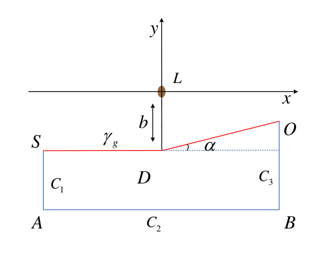 Figure 1
Peer Reviews
No public reviews on file for this paper yet. If you reviewed it on a platform where reviews are public (OpenReview, ICLR, NeurIPS, ICML), you can paste yours below so the community can read it here.
Videos
No videos yet. Explain this paper in a talk, walkthrough, or lecture? Add one.
Equivalence of Gibbons-Werner method to geodesics method in the study of gravitational lensing
Zonghai Li
School of Physical Science and Technology, Southwest Jiaotong University, Chengdu 610031, China
Center for Theoretical Physics, School of Physics and Technology, Wuhan University, Wuhan 430072, China
Tao Zhou
School of Physical Science and Technology, Southwest Jiaotong University, Chengdu 610031, China
Abstract
The Gibbons-Werner method where the Gauss-Bonnet theorem is applied to study the gravitational deflection angle has received much attention recently. In this paper, we study the equivalence of the Gibbons-Werner method to the standard geodesics method, and it is shown that the geodesics method can be derived with the Gibbons-Werner method, for asymptotically flat case. In the geodesics method, the gravitational deflection angle of particle depends entirely on the geodesic curvature of the particle ray in the Euclidean space. The gravitational deflection of light in Kerr-Newman spacetime is calculated by different technologies under the Gibbons-Werner framework, as an intuitive example to show the equivalence.
pacs:
98.62.Sb, 95.30.Sf
I Introduction
Gravitational lensing plays an important role in gravitational theory. In theoretical physics, it is used to test the fundamental theory of gravity, where a famous example is that Eddingtonet al. DED1920 ; Will2015 verified Einstein’s general relativity by means of the deflection experiment of light in the solar gravitational field 100 years ago. In astrophysics and cosmology, it is used to measure the mass of galaxies and clusters Hoekstra2013 ; Brouwer2018 ; Bellagamba2019 , and to detect dark matter and dark energy Vanderveld2012 ; cao2012 ; zhanghe2017 ; Huterer2018 ; SC2019 . In mathematics, it is related to singularity theory, topology and Finsler geometry GW2008 ; Gibbons2009-1 ; Gibbons2009-2 ; Caponio2016 ; Werner2012 .
Recently, Gibbons and Werner GW2008 introduced an elegant geometrical method of deriving the bending angle of light in a static and spherically symmetric spacetime. They used the famous Gauss-Bonnet (GB) theorem to a surface defined by the corresponding optical metric. Later, Werner Werner2012 extended this method to the rotating and stationary spacetimes. In stationary spacetimes, the optical geometry is defined by the Randers-Finsler metric. Thus, Werner applied Nazım’s method to construct an osculating Riemannian manifold where one can easily use the GB theorem. The work by Gibbons and Werner promotes the study of light deflection. On one hand, Jusufi et al. Jus-161 ; Jus-171 ; Jus-172 ; Jus-173 ; Jus-174 ; Jus-175 ; Jus-181 ; Jus-182 ; Jus-183 ; Jus-184 ; Jus-185 ; Jus-186 ; Jus-187 ; Jus-191 ; Jus-a1 ; zhu2019 studied the gravitational lensing not only in asymptotically flat spacetime but also in nonasymptotically flat spacetime such as a spacetime with cosmic string. Similar works can also be found in Refs. SO-B2 ; OSS2018 ; Arakida2018 ; OV2018 ; Goulart2018 ; Javed2019 ; AO2019 ; Leon2019 . On the other hand, Ishihara et al. ISOA2016 ; IOA2017-1 ; IOA2017-2 ; IOA2018 ; IOA2019 studied the finite-distance corrections for gravitational deflection of light both for the weak and the strong deflection limit, where the source and observer are no longer assumed to be infinitely far apart from a lens. For a review on finite-distance corrections, we refer the reader to Ref. OA2019 .
It is well known that there are many massive particles in our Universe, such as massive neutrinos. The study of gravitational deflection of massive particles allows one to understand the properties of the sources and these particles. In fact, the study of the massive particles lensing using traditional methods can be found in Refs. AR2002 ; AP2004 ; Bhadra2007 ; Yu2014 ; He2016 ; He2017a ; He2017b ; Jia2016 ; Jia2019 . Moreover, two other routes have been established by applying the GB theorem to study the gravitational deflection of massive particles. The first route is related to the Jacobi metric of curved spacetime. To be precise, one can calculate the deflection angle of massive particles via applying the GB theorem to the surface defined by the Jacobi metric Gibbons2016 ; LHZ2019 for static spacetime and by the Jacobi-Maupertuis Randers-Finsler metric Gibbons2019 for stationary spacetime. The second route is related to the optical media method. For static and spherically symmetric spacetime, Crisnejo and Gallo CG2018 used the GB theorem to study the gravitational deflections of light in a plasma medium and the deflection angle of massive particles. The finite-distance corrections of light with a plasma medium and the gravitational deflection of charged massive particles were studied quite recently CG2019 ; CGV2019 . For rotating and stationary spacetimes, Jusufi Jus-massive1 used the GB theorem to study the deflection angles of massive particles by the Kerr black hole and the Teo wormhole, respectively, based on the corresponding isotropic type metrics, the refractive index of the corresponding optical media. Furthermore, the method in Ref. Jus-massive1 was extended to distinguish naked singularities and Kerr-like wormholes Jusufi2019-1 , and to study the gravitational deflection of charged particles in Kerr-Newman spacetime Jusufi2019-2 .
In this paper, the method with the GB theorem to study the deflection angle shall be called the Gibbons-Werner method. It is worth investigating whether the Gibbons-Werner method GW2008 is equivalent to the standard geodesics method Weinberg1972 . In fact, this topic has been discussed by some researchers. The first-order equivalence has been shown in Refs. Jus-172 ; Jus-173 ; Jusufi2019-1 ; Jus-a1 , and the second-order equivalence has been shown in Refs. CG2018 ; LHZ2019 . From a conceptual point of view, however, the two methods seem to be completely different. The Gibbons-Werner method shows that the deflection of particles (photon and massive particles) is determined by a quantity outside of itself relative to the lens Werner2012 ; Jus-massive1 , and thus the gravitational deflection angle can be regarded as a global topological effect, whereas the geodesics method is usually associated within a region from particles ray to lens. In the present paper, we will demonstrate the equivalence between the Gibbons-Werner method and the geodesics method for asymptotically flat spacetime, in terms of results and concepts. More specifically, the weak gravitational deflection of light in Kerr-Newman spacetime will be taken as a simple example.
This paper is organized as follows. In Sec. II, we review the GB theorem and use the theorem to the lens geometry. Then, we show that the equivalence of the Gibbons-Werner method to geodesics method. In Sec. III, we give the Kerr-Newman spacetime as an example to show the equivalence. Finally, we summarize our results in Sec. IV. Throughout this paper, we use the natural units where and the metric signature .
II The Equivalence between the Gibbons-Werner Method and Geodesics Method
II.1 The Gauss-Bonnet theorem
Let be a compact oriented two-dimensional Riemannian manifold with the Euler characteristic and Gaussian curvature , and its boundary is a piecewise smooth curve with geodesic curvature . Then, the GB theorem states that GW2008 ; Carmo1976 :
[TABLE]
where is the area element of the surface, is the line element along , and is the exterior angle defined for the th vertex in the positive sense.
II.2 Application the Gauss-Bonnet theorem to the lens geometry
Assume be a two-dimensional smooth manifold with coordinates and a Riemannian metric . Now one can apply the GB theorem to the lens geometry in a region . For convenience, is required to be asymptotically Euclidean and thus both the particle source and the observer are in the asymptotically Euclidean region. Let with the particle ray and three curves . is described by the impact parameter , and the curves are defined by
[TABLE]
with the constant . Since the lens is excluded in the domain , . Additionally, as , boundary curve intersections , , and are in the asymptotically Euclidean region, and thus one can have , , and with the deflection angle . Then the GB theorem becomes
[TABLE]
Thus, the gravitational deflection angle can be written as
[TABLE]
as shown in Fig. 1.
II.3 The equivalence between the Gibbons-Werner method and geodesics method
In the discussion above, the Riemannian space is somewhat arbitrary, which is asymptotically Euclidean and the condition of using the GB theorem is required. In the following, three cases will be discussed to show the equivalence between the Gibbons-Werner method and the geodesics method.
II.3.1 Case 1: , and
In this case, the particle ray is a spatial geodesic in , and Eq. (3) becomes
[TABLE]
Indeed, this is the original consideration of Gibbons and Werner GW2008 ; Werner2012 and for convenience we shall call it the narrow Gibbons-Werner method. In fact, many studies fall into this category. For light deflection, one has , where is the corresponding optical metric of curved spacetime. For massive particles, , where is the corresponding Jacobi metric of curved spacetime. In stationary spacetime, the optical metric (or Jacobi metric) is a Randers-Finsler metric. However, in these cases one can use the osculating Riemannian metric by Werner’s method Werner2012 or use Jusufi’s method to avoid the Finsler metric Jus-massive1 .
II.3.2 Case 2: , and
Now, the particle ray is not geodesic in a curved space, and Eq. (3) can be written as
[TABLE]
where
[TABLE]
In Refs. IOA2017-2 ; IOA2018 ; IOA2019 , Ono et al. considered the so-called generalized optical metric space as the lens background, and used Eq. (5) to study the deflection angle of light in stationary spacetimes.
II.3.3 Case 3: , and
In this case, we assume that is Euclidean space, and Eq. (3) arrives at
[TABLE]
To our best knowledge, Eq. (6) has not been considered yet, and next it will be proved that this result is the same with the expression in the geodesics method.
The line element of a three-dimensional Euclidean space is
[TABLE]
and a unit vector normal to the plane is . The particle ray can be denoted by , and one can define its unit tangent vector as
[TABLE]
where ′ denotes derivative with respect to . Therefore,
[TABLE]
and one can obtain the geodesic curvature of in the plane as follows Carmo1976 :
[TABLE]
Then, one can calculate the deflection angle by
[TABLE]
which is nothing but the formula of calculating deflection angle with geodesics method in Refs. He2016 ; He2017a ; He2017b .
In short, the geodesics method just corresponds to special cases for the Gibbons-Werner method, where the GB theorem is used to Euclidean space. In other words, the geodesics method categorizes the deflection angle into the influence of geodesic curvature of particles moving in Euclidean space. Therefore, the geodesics method also has geometric meaning from the perspective of curvature.
III An example: the deflection of light in Kerr-Newman spacetime
For the second-order post-Minkowskian approximation, the components of the metric of the Kerr-Newman spacetime in the harmonic coordinates can be written as Lin2014 ; Yang2019
[TABLE]
where and are the mass and electric charge of the Kerr-Newman black hole, respectively. , and is the th component of the gravitational vector potential , where is the angular momentum per unit mass. is the Kronecker symbol and the expanding parameter represents the black hole parameters , or . The above metric is expanded as the power series of the parameters , and , and is the series with order greater than , such as .
For stationary spacetime, its optical geometry defined by the Randers-Finsler metric takes the form Werner2012 ; Chern2002
[TABLE]
where is a Riemannian metric and is a one-form satisfying . Consider a null curve in the Kerr-Newman spacetime, , and one can find a Randers-Finsler metric,
[TABLE]
where
[TABLE]
III.1 Werner’s method: ,
In this subsection, we will apply Werner’s method Werner2012 to calculate the gravitational deflection angle of light. The light ray is geodesic in Randers-Finsler space, and therefore, Eq. (4) can be considered. To simplify, one can study the null geodesic in the equatorial plane. Chose as the equatorial plane, and one can find the Kerr-Newman-Randers black hole optical metric as follows
[TABLE]
where and are the same as those in Eq. (III) except that and only run in here.
The Randers-Finsler metric is characterized by the Hessian Chern2002 ; Werner2012
[TABLE]
where , and with the tangent space at a given point. In order to obtain a Remannian metric , one can choose a smooth nonzero vector field over that contains the tangent vectors along the geodesic such that , defining
[TABLE]
In this construction, we can obtain a crucial result that the geodesic of is also a geodesic of , i.e., Werner2012 .
Following Werner Werner2012 , the osculating Riemannian manifold can be used to calculate the gravitational defection angle of light. Near the undeflected light rays He2016 ; He2017a , one can choose the vector field as
[TABLE]
Using Eqs. (16), (17), and (III.1), finally the osculating Riemannian metric can be obtained as follows:
[TABLE]
with the determinant up to second order
[TABLE]
and the Gaussian curvature
[TABLE]
In harmonic coordinates, Eq. (4) can be written as
[TABLE]
Here denotes the light ray up to first order (see the Appendix A)
[TABLE]
Substituting Eqs. (22), (23) and (25) into Eq. (24), one can get the second-order deflection angle of light as follows:
[TABLE]
which is consistent with the results in Ref. He2017a .
III.2 The generalized optical metric method: , and
In this section we consider the Riemannian space defined by . The line element of is given by
[TABLE]
The light ray is the spatial curve in and following Fermat’s principle, the motion equation of light ray is IOA2017-2
[TABLE]
where , denotes the Christoffel symbol associated with , and denotes the covariant derivative with . The existence of illustrates that the orbit of light is not the geodesic in . Naturally, the contribution of geodesic curvature should be considered and we will use Eq. (5) to calculate the deflection angle. We focus on the motion of the light in the equatorial plane . Then the geodesic curvature of curve is given by IOA2017-2
[TABLE]
where is the Levi-Civita tensor and is a unit normal vector for the equatorial plane. Then, choose the unit normal vector as , and one can obtain
[TABLE]
where has been used and the comma denotes the partial derivative. With Eqs. (III) and (30), one can have
[TABLE]
where the first-order light ray in Eq. (25) has been used.
According to Eq. (5), the deflection angle of the light can be divided into two parts. First, the Gauss curvature of is
[TABLE]
and one can calculate the part associated with Gauss curvature
[TABLE]
Second, from Eqs. (25) and (31), the part associated with geodesic curvature is
[TABLE]
Finally, the total deflection angle can be obtained as follows:
[TABLE]
which is consistent with the result in Eq. (26).
III.3 The geodesics method: ,
From second-order light ray in Eq. (40), the following relation can be obtained
[TABLE]
The deflection angle can be obtained by Eq. (6)
[TABLE]
Certainly, this expression is the same as the result obtained by Werner’s method in Eq. (26) and by the generalized optical metric method in Eq. (35).
IV conclusion
In this work, we investigate the equivalence of the Gibbons-Werner method to the geodesics method in the study of gravitational lensing. It is shown that the geodesics method can be derived with the Gibbons-Werner method for asymptotically flat spacetime. In the Gibbons-Werner procedure, one can choose the Euclidean space as the lens background and the deflection effect is completely determined by the geodesic curvature of the particle’s trajectory. Thus, one can choose arbitrary asymptotically Euclidean space as the lens background and the deflection angle can be written as . The difference between these different background spaces is that the contribution on and is different. However, the total deflection angle is always constant. In practice, it is more convenient to use the geodesics method or the narrow Gibbons-Werner method. We can illustrate these two methods using the following formula
[TABLE]
The left side of the equation represents the geodesic method , while the right side represents the narrow Gibbons-Werner method .
As an example to show the equivalence, we calculate the second-order gravitational deflection angle of light in Kerr-Newman spacetime, for three options with the Gibbons-Werner method, in the harmonic coordinates. More, the harmonic coordinates bring a lot of simplicity and overcome the cumbersome iterative in Ref. LHZ2019 .
Acknowledgements.
This work was supported by the National Natural Science Foundation of China under Grants No. 11405136 and No. 11847307, and the Fundamental Research Funds for the Central Universities under Grant No. 2682019LK11.
Appendix A Second-order light orbit
In this Appendix, we calculate the second-order light ray in Kerr-Newman spacetime. For the photon, the velocity , and thus Eq. (11) in the literature He2017a reads
[TABLE]
where is the affine parameter in Kerr-Newman spacetime. With the boundary conditions He2017a , one can get
[TABLE]
Finally, with the first-order parameter transformation He2017a and integrating , one can get the second-order light ray as follows:
[TABLE]
where we have considered the boundary conditions He2017a .
The reference list from the paper itself. Each links out to its DOI / PubMed record.
- 1(1) F. W. Dyson, A. S. Eddington, and C. Davidson, Phil. Trans. R. Soc. A 220 , 291 (1920).
- 2(2) C. M. Will, Classical Quantum Gravity 32 , 124001 (2015).
- 3(3) H. Hoekstra, M. Bartelmann, H. Dahle, H. Israel, M. Limousin, and M. Meneghetti, Space Sci. Rev. 177 , 75 (2013).
- 4(4) M. M. Brouwer et al. , Mon. Not. R. Astron. Soc. 481 , 5189 (2018).
- 5(5) F. Bellagamba et al. , Mon. Not. R. Astron. Soc. 484 , 1598 (2019).
- 6(6) R. A. Vanderveld, M. J. Mortonson, W. Hu, and T. Eifler, Phys. Rev. D 85 , 103518 (2012).
- 7(7) H. J. He and Z. Zhang, J. Cosmol. Astropart. Phys. 08 (2017) 036.
- 8(8) S. Cao, G. Covone, and Z. H. Zhu, Astrophys. J. 755 , 31 (2012).