Risk-neutral option pricing under GARCH intensity model
Kyungsub Lee

TL;DR
This paper explores a risk-neutral option pricing approach using a GARCH intensity model that captures key features of financial returns like volatility clustering and leverage effects, offering flexible volatility adjustments.
Contribution
It introduces a novel GARCH intensity model for option pricing that accounts for complex return dynamics and adapts volatility under different probability measures.
Findings
Model captures volatility clustering and leverage effects.
Flexible volatility adjustment under measure change.
Enhances accuracy of option pricing models.
Abstract
The risk-neutral option pricing method under GARCH intensity model is examined. The GARCH intensity model incorporates the characteristics of financial return series such as volatility clustering, leverage effect and conditional asymmetry. The GARCH intensity option pricing model has flexibility in changing the volatility according to the probability measure change.
Click any figure to enlarge with its caption.
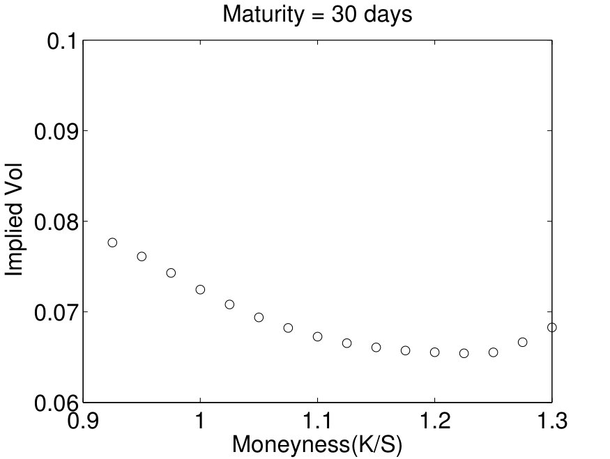 Figure 1
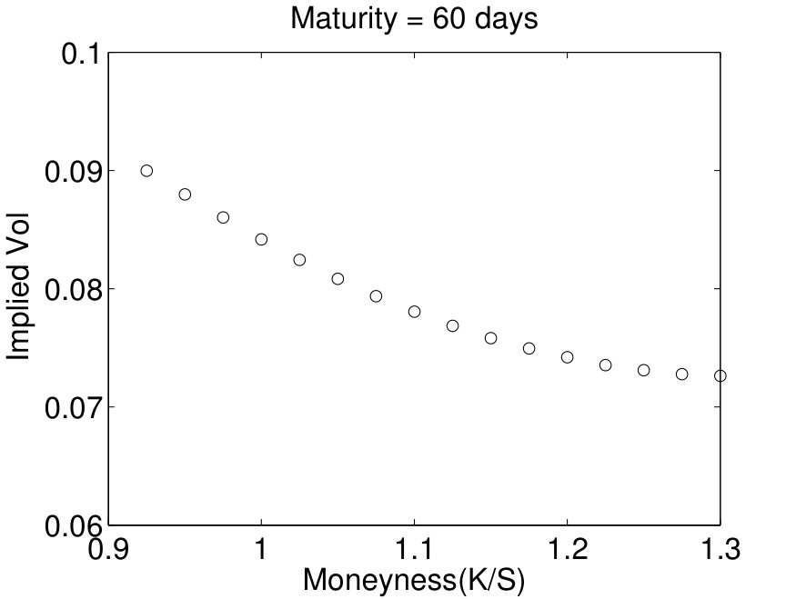 Figure 2
Peer Reviews
No public reviews on file for this paper yet. If you reviewed it on a platform where reviews are public (OpenReview, ICLR, NeurIPS, ICML), you can paste yours below so the community can read it here.
Videos
No videos yet. Explain this paper in a talk, walkthrough, or lecture? Add one.
Risk-neutral option pricing under GARCH intensity model
Kyungsub Lee111Department of Statistics, Yeungnam University, Gyeongsan, Gyeongbuk 38541, Korea
Abstract
The risk-neutral option pricing method under GARCH intensity model is examined. The GARCH intensity model incorporates the characteristics of financial return series such as volatility clustering, leverage effect and conditional asymmetry. The GARCH intensity option pricing model has flexibility in changing the volatility according to the probability measure change.
1 Introduction
This paper develop the risk-neutral option pricing framework under the GARCH intensity model. The financial asset returns series have interesting characteristics. Large volatility tends to follow large volatility and small volatility tends to follow small volatility in the series of financial returns and this is called volatility clustering. The leverage effect indicates that today’s volatility has a negative correlation with past returns. Conditional asymmetry is an asymmetric correlation between current and past volatility, depending on whether the current and past returns are positive or negative.
These characteristics are well captured by various GARCH models. The volatility clustering is well described by original GARCH model [4]. [13], [12], [8], and [14] incorporate the leverage effects and [1] capture the conditional asymmetry. The GARCH intensity model introduced by [5] also describes the volatility clustering, leverage effect and conditional asymmetry in financial asset price dynamics and based on Poisson type intensity processes.
The risk-neutral option pricing is a method to determine a no-arbitrage prices of financial options with underlying assets. The option pricing theory of [3] and [11] is based on the risk-neutral pricing framework. The relation between risk-neutral pricing and the no-arbitrage principle was studied by [9] and [10]. [6] explained the risk-neutral option pricing under the GARCH model. This paper extends the risk-neutral pricing idea to the GARCH intensity model.
The remainder of the paper is organized as follows: Section 2 reviews the GARCH intensity model. Section 3 examines the mathematical analysis on the risk-neutral option pricing under the GARCH intensity model. Section 4 extends the option pricing theory to the generalized GARCH intensity model. Section 5 concludes the paper.
2 GARCH intensity model
First, we review the GARCH intensity model introduced by [5]. In the model, the asset price process movement is described by two Poisson-type processes with time-varying intensity processes. A probability space with a filtration , , is given.
Assumption 2.1** ([5]).**
We are given -adapted r.c.l.l. processes , and positive -adapted r.c.l.l. processes , for satisfying the following conditions:
(i) (Discrete observation time) and , .
(ii) (Conditional distribution) has Poisson distribution with intensity , . Hence
[TABLE]
(iii) (Conditional independence) and are conditionally independent given , .
(iv) (Step process) and , .
(v) (Predictability) depends on and , , and similarly for .
(vi) (Asset price) With a constant , the price process is
[TABLE]
With a price jump at time , or depending on the direction of the jump. The asset price can also be represented by a stochastic differential equation given by
[TABLE]
Let
[TABLE]
be the log-return over the period . Then the integer-valued random variable defined by
[TABLE]
has the conditional Skellam distribution on
[TABLE]
where is the modified Bessel function of the first kind defined by
[TABLE]
Since the closed form of conditional probability density is exist, the maximum likelihood estimation can be easily employed.
Definition 2.2** (Decomposition of Log-Return).**
Define , , by
[TABLE]
Recall that under Assumption 2.1,
[TABLE]
and
[TABLE]
where is a drift term, is an Itô correction factor, and is a -measurable shock occurred during time interval .
As in [5], to capture volatility clustering, GARCH[4]-type modeling is applied:
[TABLE]
for some constants and . If
[TABLE]
in the GARCH intensity model, then the GARCH-type time varying volatility is obtained. To show this, let be a one-step-ahead conditional variance of return at , then
[TABLE]
and
[TABLE]
This is consistent with conditional variance modeling in GARCH. In addition, we also consider the GJR[8] GARCH-type intensity model:
[TABLE]
where
[TABLE]
3 Risk-neutral option pricing
We propose an option pricing method for intensity models by constructing an equivalent measure under which the discounted stock price process is a martingale. We assume that the underlying asset pays no dividend and let be the risk-free interest rate. In the following we choose new intensities for an equivalent martingale measure.
Definition 3.1**.**
Take a pair of positive r.c.l.l. adapted step processes and such that
[TABLE]
(We take the right hand side equal to since the left hand side is regarded as drift under a risk-neutral measure.)
(i) Let
[TABLE]
for , and let and for define
[TABLE]
(ii) Let and for define
[TABLE]
Theorem 3.2**.**
* is a -martingale.*
Proof.
For , define and by and
[TABLE]
Then
[TABLE]
(For the details of the proof, see [7].) Since are martingales, are martingales for and hence
[TABLE]
Note that
[TABLE]
Since and are conditionally independent given , we have
[TABLE]
Take such that and . Then
[TABLE]
and
[TABLE]
∎
Definition 3.3**.**
Define an equivalent probability measure by
[TABLE]
Now we change intensities.
Lemma 3.4**.**
The intensities of and under are given by and , respectively.
Proof.
Since has a Poisson distribution for , we have
[TABLE]
for an -measurable random variable . We will show that the same relation holds for and . Define as in the proof of Theorem 3.2. For a constant , we have
[TABLE]
where the last expression is the moment generating function of a Poisson distribution with intensity . For , the proof is identical. ∎
As in Definition 2.2 we define and in terms of , and .
[TABLE]
Then
[TABLE]
Theorem 3.5**.**
The discounted stock price process is a -martingale, i.e., for
[TABLE]
Proof.
By the tower property it suffices to consider the case that . Since have intensities under , we have
[TABLE]
∎
Basically the GARCH intensity option pricing model has flexibility in changing the volatility according to the measure change. This allows us to construct a GARCH intensity option pricing model consistent with volatility spread [2].
If we consider a special case when and satisfy an additional condition
[TABLE]
Since , we have
[TABLE]
Since is the conditional variance of under given , we have
[TABLE]
for . We plot implied volatility smile in Figure 1. Using the parameter setting in Table 1 in Monte Carlo method, we generate sample price paths. The implied volatility is obtained using Black-Scholes-Merton model. The left panel is for the implied volatility with 30 days maturity and the right panel is for 60 days maturity.
Remark 3.6**.**
Assume that and for some constants and for every , and assume that the European call option price at time is given by
[TABLE]
where is the conditional variance preserving measure. By It̂o’s formula, we have
[TABLE]
where
[TABLE]
Note that , and are -martingales. Hence is a martingale, and the integrand should be zero. Thus satisfies
[TABLE]
For small , consider the following approximations:
[TABLE]
Then
[TABLE]
and by Eqs. (2) and (3), we obtain Black-Scholes-Merton PDE
[TABLE]
where .
4 A generalization of GARCH intensity model
The goal of this section is to provide the generalized version for the previous model in which it is assumed to be that the sizes of stock price changes affected by news are represented by independent and identically distributed random variables.
Assumption 4.1**.**
The assumptions (i)–(v) for asset price process are the same as in Assumption 2.1(i)–(v) and we need an additional condition:
(vi) (Asset price) The asset price satisfies
[TABLE]
for some i.i.d. random variables and , .
Lemma 4.2**.**
Under Assumption 4.1, we have
[TABLE]
and
[TABLE]
where
[TABLE]
and
[TABLE]
Proof.
Recall that
[TABLE]
Now use the fact that each conditional distribution
[TABLE]
is a compound Poisson distribution. ∎
Note that depending on distributions of and , the model allows the skewness in the conditional distribution of log-return . For example, if the tail of the distribution of is fatter than the tail of the distribution of , then the conditional distribution of log-return is negatively skewed.
Definition 4.3**.**
We define
[TABLE]
where
[TABLE]
respectively.
Note that, by direct computation, we have
[TABLE]
The mean correction factor appears because we model with log-return and this implies that
[TABLE]
and using the property of compound Poisson distributions, we have
[TABLE]
The one step ahead expectation of future stock price can be represented as exponential of drift term multiplied by current stock price, that is
[TABLE]
The derivation of equivalent martingale measure for extended version of GRACH intensity model is similar to the previous version.
Definition 4.4**.**
Let be probability density functions of , respectively and are some probability density functions (which are desired probability density functions of under equivalent martingale measure).
(i) Let
[TABLE]
and and be two r.c.l.l. adapted step processes satisfying the equation
[TABLE]
for each , and
[TABLE]
for .
(ii) Suppose that and are positive processes. Let
[TABLE]
[TABLE]
for integer . Define
[TABLE]
and
[TABLE]
for , recursively.
Remark 4.5**.**
Note that -measurable random variable is zero when the conditional variance of return distribution of the martingale measure is equal to the variance under physical measure. depends on random variables and .
Lemma 4.6**.**
For ,
[TABLE]
Proof.
For , define
[TABLE]
[TABLE]
Then and are -measurable and satisfy
[TABLE]
and
[TABLE]
Note that
[TABLE]
Since and are conditionally independent upon , we have
[TABLE]
Finally, for , we have
[TABLE]
∎
Since , we use in Definition 4.4 to construct a new probability measure . We define
[TABLE]
Lemma 4.7**.**
Under the measure in (6), for every , the conditional distributions
[TABLE]
and
[TABLE]
are Poisson distributions with new intensities and , respectively. Moreover, have probability density function under .
Proof.
Define as in the proof of Lemma 4.6. For a constant , we have
[TABLE]
and
[TABLE]
Put
[TABLE]
and let be the conditional moment generating function of , i.e.
[TABLE]
Note that
[TABLE]
Then
[TABLE]
Note that
[TABLE]
which is the moment generating function of a Poissson distribution with intensity . Hence is a Poissson distribution with intensity . For , the proof is the same.
For the remaining part of lemma, to figure out the distribution of under , it is enough to check the distribution of under . Without loss of generality, assume that first jump, i.e. the occurrence time of random variable is less than . Thus, for a constant , we have
[TABLE]
The last equality holds since given random variables independent and since
[TABLE]
Furthermore, because of independency and the fact that
[TABLE]
(by Lemma 4.6 when is constant) and
[TABLE]
for each . Finally we have
[TABLE]
which implies has a probability density function under . For general , the proof is the same. ∎
The choice for risk-neutral distributions and are related to the skewness in conditional distribution of log-return under risk-neutral measure. This is similar to the fact that distributions and are related to the skewness under physical measure. Now we show that under the equivalent martingale measure , the discounted stock price process is a martingale.
Theorem 4.8**.**
Under the measure defined by (6), we have
[TABLE]
for .
Proof.
Take such that .
[TABLE]
Let be the conditional moment generating function of
[TABLE]
given filtration . Then
[TABLE]
where is defined in Definition 4.4. Hence
[TABLE]
and
[TABLE]
The last equality is due to Definition 4.4(i). By applying the tower property, we obtain the desired result for arbitrary and . ∎
5 Concluding remark
The risk-neutral option pricing framework for the GARCH intensity model was introduced. Equivalent martingale measures are provided and hence the the risk-neutral option price is computed under the measure. The framework is consistent with the empirical characteristics such as volatility smile and spread. The theory is easily extended to the generalized version of the GARCH intensity model.
The reference list from the paper itself. Each links out to its DOI / PubMed record.
- 1[1] Babsiri, M. E., and Jean-Michel Zakoian. 2001. Journal of Econometrics 101 :257 – 294.
- 2[2] Bakshi, G., and Dilip Madan. 2006. Management Science 52 :1945–1956.
- 3[3] Black, F., and Myron S. Scholes. 1973. Journal of Political Economics 81 :637–654.
- 4[4] Bollerslev, T. 1986. Journal of Econometrics 31 :307–327.
- 5[5] Choe, G. H., and Kyungsub Lee. 2014. A St A Advances in Statistical Analysis 98 :197–224.
- 6[6] Duan, J.-C. 1995. Mathematical Finance 5 :13–32.
- 7[7] Elliott, R. J., and P. Ekkehard Kopp. 1990. Stochastic Analysis and Applications 8 :157 – 167.
- 8[8] Glosten, L. R., Ravi Jagannathan, and David E. Runkle. 1993. Journal of Finance 48 :1779–1801.