Network Lifetime Maximization in Wireless Mesh Networks for Machine-to-Machine Communication
Emma Fitzgerald, Micha{\l} Pi\'oro, Artur Tomaszewski

TL;DR
This paper introduces new optimization methods for extending the lifetime of wireless mesh networks in IoT applications by leveraging network reconfiguration, demonstrating significant improvements through numerical simulations.
Contribution
It presents novel optimization formulations for network lifetime maximization that incorporate reconfiguration strategies suitable for heterogeneous IoT mesh networks.
Findings
Network lifetime increased by up to 75% with reconfiguration.
Few configurations needed for practical implementation.
Low synchronization and signaling overhead for reconfiguration.
Abstract
In this paper we present new optimization formulations for maximizing the network lifetime in wireless mesh networks performing data aggregation and dissemination for machine-to-machine communication in the Internet of Things. We focus on heterogeneous networks in which multiple applications co-exist and nodes may take on different roles for different applications. Moreover, we address network reconfiguration as a means to increase the network lifetime, in keeping with the current trend towards software defined networks and network function virtualization. To test our optimization formulations, we conducted a numerical study using randomly-generated mesh networks from 10 to 30 nodes, and showed that the network lifetime can be increased using network reconfiguration by up to 75% over a single, minimal-energy configuration. Further, our solutions are feasible to implement in practical…
Click any figure to enlarge with its caption.
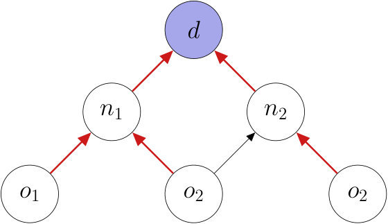 Figure 1
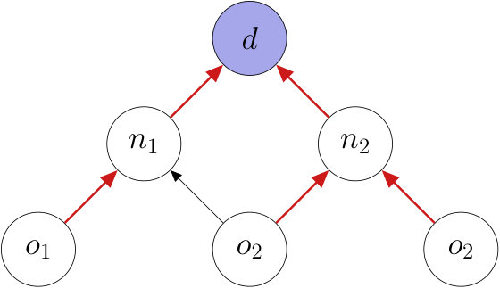 Figure 2
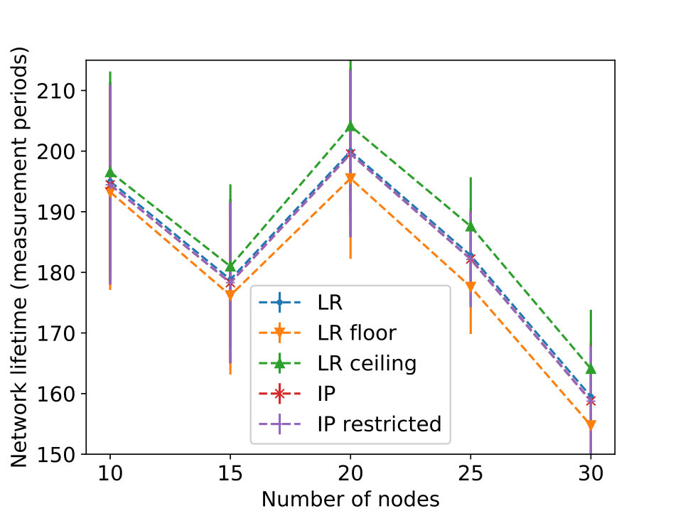 Figure 3
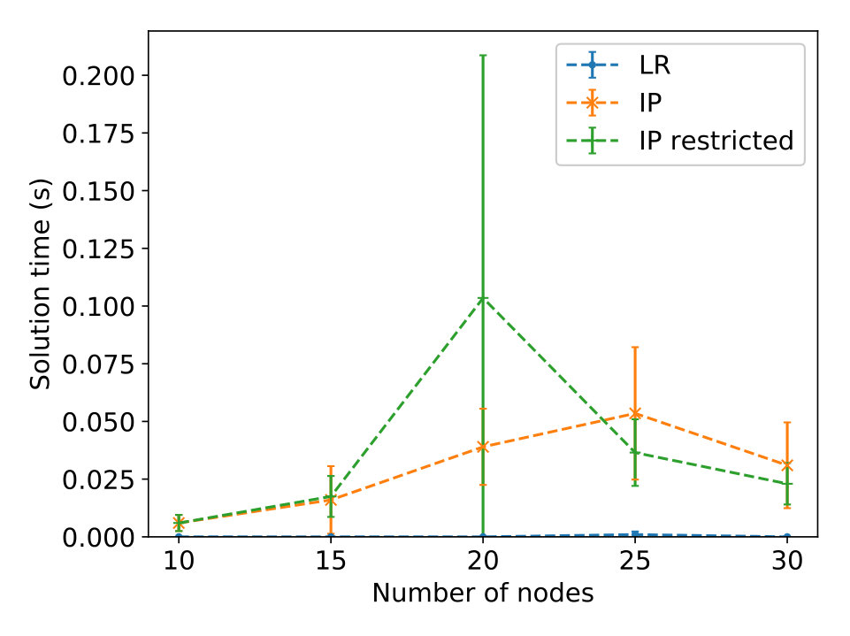 Figure 4
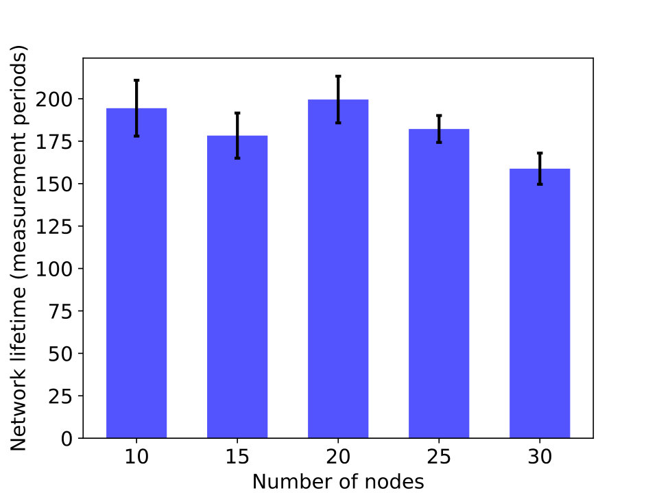 Figure 5
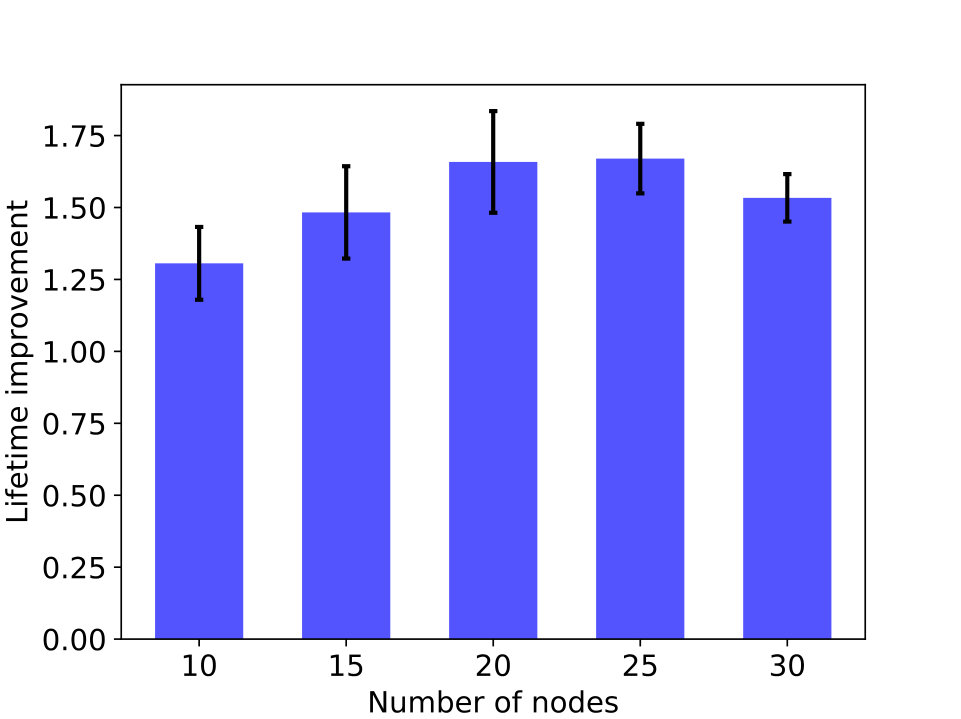 Figure 6
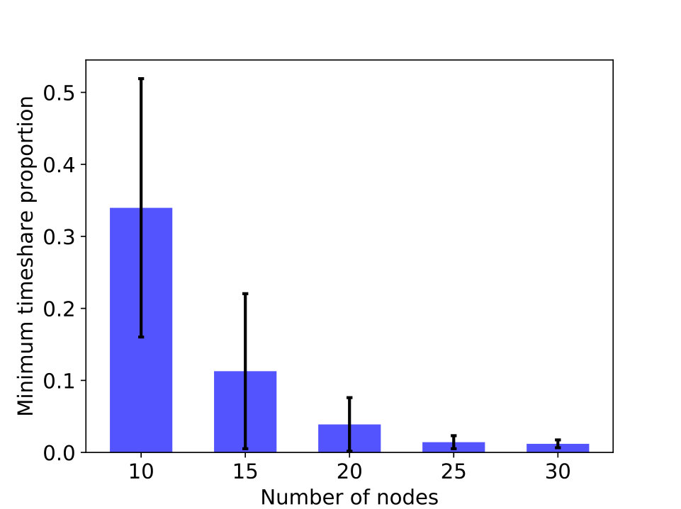 Figure 7
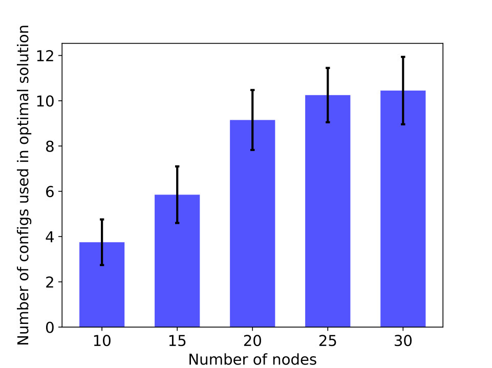 Figure 8
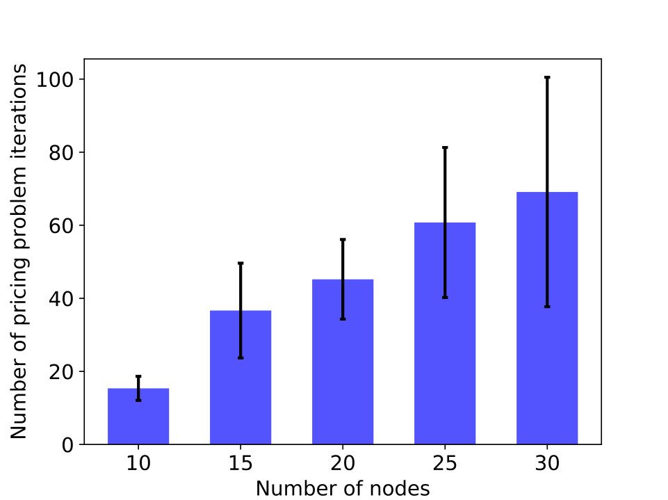 Figure 9
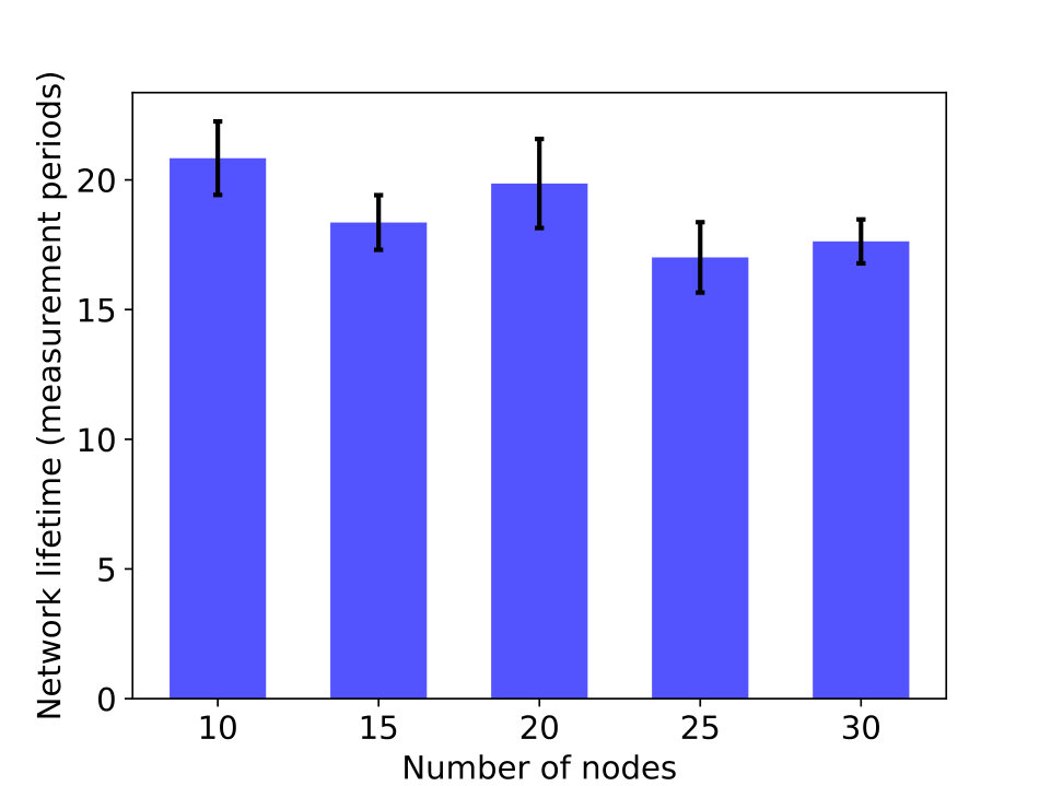 Figure 10
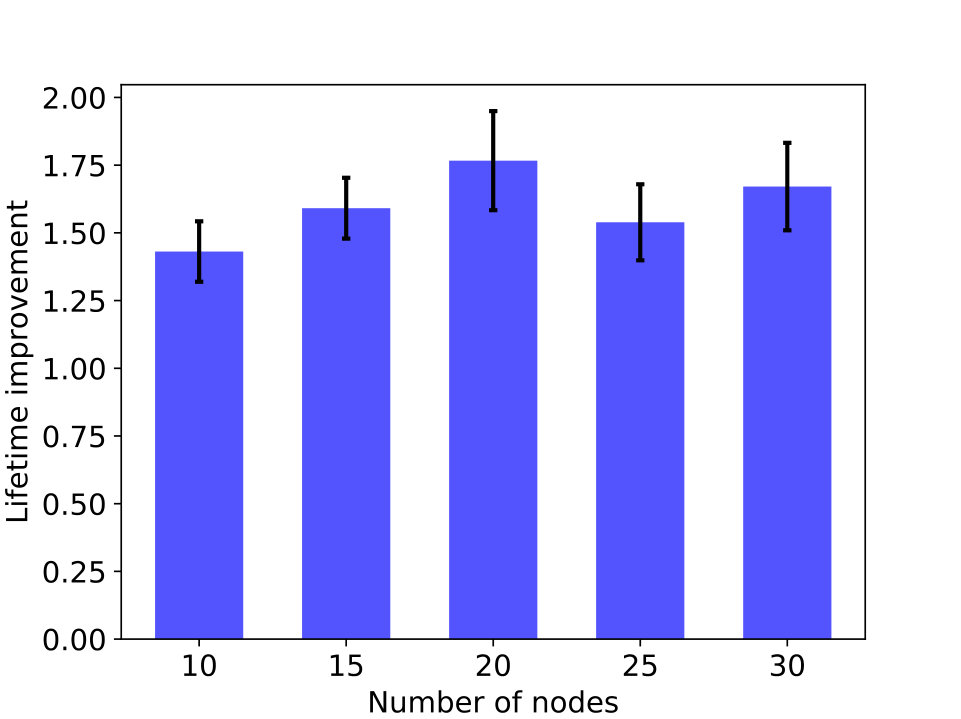 Figure 11
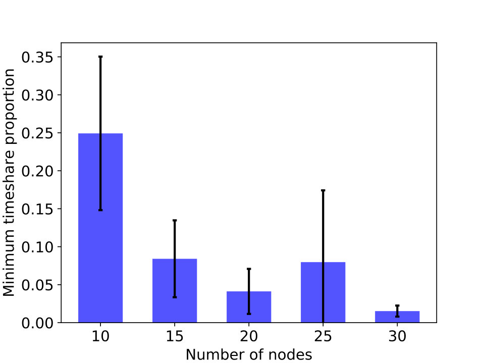 Figure 12
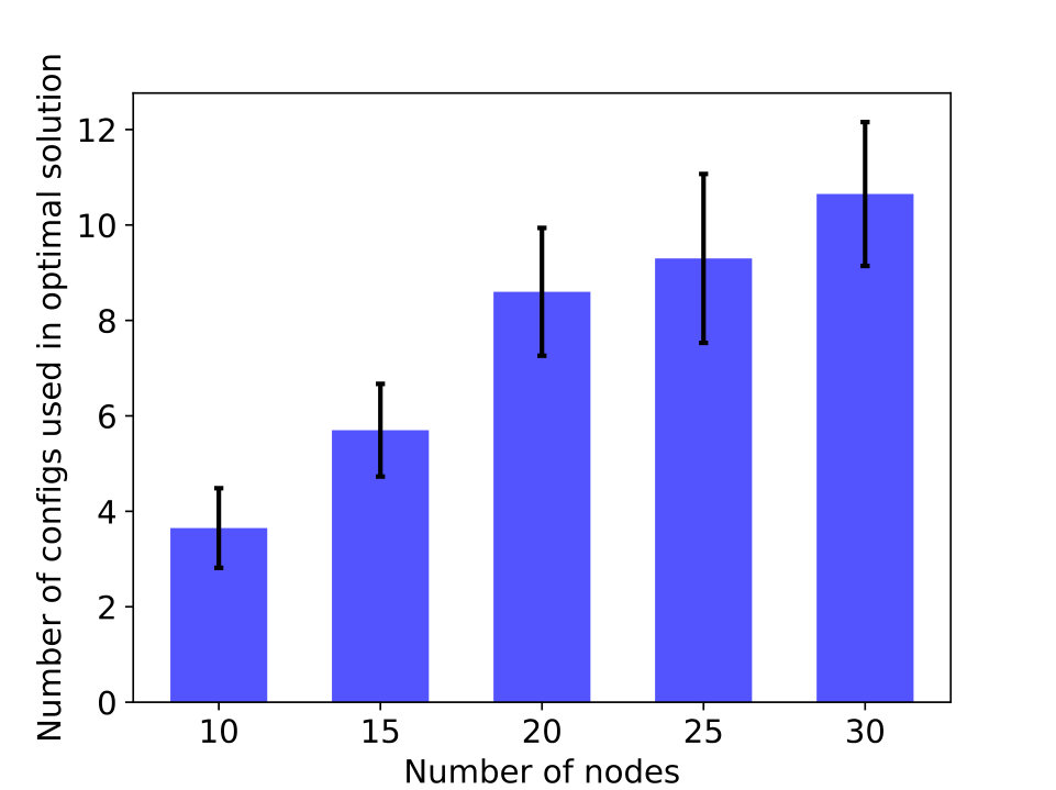 Figure 13
| set of nodes (vertices) in the network | |
|---|---|
| set of arcs , indicating node is within transmission range of node (barring any interference) | |
| set of origin (sensor) nodes | |
| set of aggregator nodes | |
| set of destination (actuator) nodes | |
| set of network configurations | |
| set of incoming arcs to node | |
| set of outgoing arcs from node | |
| timeshare of network configuration | |
| whether or not the measurement from origin is received by destination | |
| flow of the measurement from origin to destination on arc | |
| whether or not arc carries the measurement from origin | |
| whether or not arc carries an (aggregated) measurement | |
| whether or not the measurements from origins are aggregated at node | |
| energy required to broadcast from node | |
| number of (aggregated) measurements aggregated at node minus (and if there is no aggregation at ) | |
| whether or not the measurement from origin is received by any destination | |
| set of all 2-element subsets of | |
| transmission energy required on arc | |
| processing energy required for aggregation by node | |
| battery capacity of node (in J) | |
| energy used per measurement period by node in configuration (in J) | |
| battery depletion fraction per measurement period of node in configuration | |
| set of binary numbers | |
| set of real numbers | |
| set of non-negative real numbers | |
| set of non-negative integers |
| Nodes | Area width [m] | ||||
|---|---|---|---|---|---|
| 10 | 122.47 | 3 | 4 | 2 | 4 |
| 15 | 150.0 | 5 | 6 | 3 | 6 |
| 20 | 173.21 | 6 | 8 | 3 | 9 |
| 25 | 193.65 | 8 | 10 | 4 | 9 |
| 30 | 212.13 | 9 | 12 | 5 | 13 |
Peer Reviews
No public reviews on file for this paper yet. If you reviewed it on a platform where reviews are public (OpenReview, ICLR, NeurIPS, ICML), you can paste yours below so the community can read it here.
Videos
No videos yet. Explain this paper in a talk, walkthrough, or lecture? Add one.
Taxonomy
TopicsEnergy Efficient Wireless Sensor Networks · IoT and Edge/Fog Computing · IoT Networks and Protocols
Network Lifetime Maximization in Wireless Mesh Networks for Machine-to-Machine Communication
Emma Fitzgerald
Michał Pióro
Artur Tomaszewski
Department of Electrical and Information Technology, Lund University, Lund, Sweden
Institute of Telecommunications, Warsaw University of Technology, Warsaw, Poland
Abstract
In this paper we present new optimization formulations for maximizing the network lifetime in wireless mesh networks performing data aggregation and dissemination for machine-to-machine communication in the Internet of Things. We focus on heterogeneous networks in which multiple applications co-exist and nodes may take on different roles for different applications. Moreover, we address network reconfiguration as a means to increase the network lifetime, in keeping with the current trend towards software defined networks and network function virtualization. To test our optimization formulations, we conducted a numerical study using randomly-generated mesh networks from 10 to 30 nodes, and showed that the network lifetime can be increased using network reconfiguration by up to 75% over a single, minimal-energy configuration. Further, our solutions are feasible to implement in practical scenarios: only few configurations are needed, thus requiring little storage for a standalone network, and the synchronization and signalling needed to switch configurations is low relative to each configuration’s operating time.
keywords:
network lifetime; machine-to-machine communication; aggregation; integer programming
††journal: Ad Hoc Networks
1 Introduction
In an increasingly wireless world, and in particular with the rise of the Internet of Things, energy efficiency for end devices is a critical component in enabling new applications. Taking an application-centric view, it is not the energy consumption of individual nodes in the network that is the most important consideration, but rather how long the network as a whole can fulfill its intended purpose, that is, serve the demands of the application(s) running on it. This time is called the lifetime of the network.
To achieve maximum network lifetime, reconfiguration of the network, in the form of changing routing and/or which tasks are assigned to which nodes, may be necessary. For example, with a given set of paths taken by the various application data flows, some nodes may be more heavily loaded than others and become bottlenecks, needing to transmit often and draining their batteries more quickly. Once these critical nodes are out of power, the path(s) on which they lie will fail, causing a disruption in service. However, in many cases, especially for mesh networks, it is possible to find other feasible paths consisting only of nodes that still have some power remaining. In fact, to achieve the longest possible lifetime, reconfiguration of routing of traffic demands may need to be performed multiple times.
In future, especially as 5G comes into effect, such reconfiguration will become more feasible. There is currently a trend towards software-defined networking and network function virtualization, making telecommunications networks more flexible and reconfigurable. Moreover, it is typical that end devices will have a connection to cloud or edge servers, possibly through multiple different gateways, and therefore do not need to themselves have sufficient computation power to determine the optimal configuration or reconfiguration. Instead, this may be done in the cloud or the fog, and then communicated to the end devices.
In our previous work [1], we studied the problem of routing in a wireless mesh network together with data aggregation and dissemination for machine-to-machine communication, optimizing for minimal total energy usage (which can equivalently be understood as the minimal average power consumption by the network nodes). In the current paper, we now present complementary, novel optimization formulations for maximum network lifetime (i.e., the time until the network ceases to be fully operational), in which the network is able to be reconfigured both in terms of routing of traffic streams, and which nodes are selected to aggregate and/or disseminate (via multicast transmission) individual sensor measurements. We examine practical implementation issues and describe how our approach can be deployed in real networks. We also conducted a numerical study solving our optimization problems for randomly generated mesh networks with 10 to 30 nodes. Our results show that the network lifetime can be increased by up to 75% compared with configuring the network for minimum total energy usage, and that relatively few (around 10) different configurations are needed to achieve the maximum lifetime. This means that the optimal solutions we find here are feasible to implement in practice, as the overhead for reconfiguration will be low compared to the total network lifetime.
The contributions of this paper are the following.
We provide novel optimization formulations for maximizing network lifetime that allow for reconfiguration of routing and node tasks. 2. 2.
We develop a general solution approach to these optimization problems, based on column generation. This allows our approach to be applied to arbitrary network tasks. 3. 3.
We examine the specific case of machine-to-machine communication, in which sensor measurements can be aggregated within the network, and must be disseminated via multicast transmission to multiple destinations. We give an appropriate pricing problem formulation for this application. 4. 4.
Our solution approach is feasible to implement in practice, since only few configurations are used for maximal lifetime, and the requirements for signalling and synchronization needed to perform reconfiguration are low. 5. 5.
We present results from a numerical study investigating the performance of our optimization approach, and showing that it can provide large improvements in network lifetime for the considered application. We compare performance for maximum network lifetime with that for total energy minimization, and discuss the trade-offs between these two approaches. 6. 6.
We provide tight upper and lower bounds for the optimal solutions to our formulations, as well as a heuristic that closely tracks the optimal performance, and present a numerical performance evaluation for the bounds and heuristic.
The rest of this paper is organized as follows. In Section 2 we survey the related work on network lifetime. In Section 3, we describe our system model and give optimization formulations to solve for the maximum network lifetime. Section 4 details our numerical study and results for varying network sizes. Finally, Section 5 concludes this paper.
2 Related Work
In [1], we considered the problem of data aggregation and dissemination in IoT networks serving, for example, monitoring, sensing, or machine control applications. A key aspect of the IoT that differentiates it from classical wireless sensor networks (WSNs) is its heterogeneity. We therefore considered cases where nodes may take on different roles (for example, sensors, destinations, or transit nodes) for different applications, and where multiple applications with different demands may be present in the network simultaneously. Moreover, these demands can be more general than only collecting data and forwarding it to a single sink, as is usually the case for WSNs. Rather, data may be processed within the network (we take the specific case of aggregation), and may be disseminated to multiple sinks via multicast transmissions.
However, in that work, we focused on minimizing the total energy usage. We now seek to extend this to consider the network lifetime. While total energy usage may be important in, for example, green networking, in which we wish to reduce the environmental impact and thus the overall energy usage, network lifetime is a critical performance measure both for traditional WSNs and for emerging IoT networks. Network lifetime gives a measure of how long the network can operate without intervention and, in cases where it is impractical to charge nodes or change their batteries, it gives the total operating time for the network.
Network lifetime has been studied extensively in the context of WSNs since the early 2000’s. A full review of the literature in this area is therefore beyond the scope of this paper; a recent survey can be found in [2]. We will instead focus on the recent work that is most relevant to the current paper.
There are numerous different definitions of network lifetime adopted in the literature [2]. Some of these include that the network lifetime expires at the time instant a certain number (possibly as low as one) or proportion of nodes deplete their batteries, when the first data collection failure occurs, or when the specific node with the highest consumption rate runs out of energy. In [2], these definitions are classified into four categories depending on whether they are based on node lifetime, coverage and connectivity, transmission, or a combination of parameters.
However, a problem with many of these definitions is that they are not application-centric. In practice, whether or not a network is functional depends on the specific application or applications which it serves. Some applications may require all nodes in the network to have remaining energy, while others may continue to operate correctly with only a few nodes working. The lifetime also depends on the capabilities of the network. For example, if the network can be reconfigured, the lifetime may be extended by switching configurations. This can be facilitated by the use of software defined networking [3], as well as support from cloud services that are capable of performing even demanding calculations to determine the best network configuration at any given time, without incurring an energy cost in the end devices.
This is the approach we adopt in this paper, and we define valid configurations based on the demands of the applications present in the network along with the roles the various nodes play in these demands. As such, we will adopt a general definition of the network lifetime as the total time in which the network is operational. Since we consider a class of applications with data streams as their demands, this is most similar to the definition used in [4], where the network lifetime was defined as the number of sensory information task cycles achieved until the network ceases to be fully operational.
There have been numerous techniques developed to improve the network lifetime in specific use cases, mostly for WSNs consisting of homogeneous sensor nodes and a single sink. In [5], the schedule and charge amounts of a mobile vehicle that charges nodes were optimized, while in [6] nodes may regain energy through energy harvesting, and routing is then optimized to maximize the lifetime. Routing is also the focus of [7], however here an energy-balancing routing protocol is developed, rather than determining optimal routes. Multilayer optimization approaches are adopted in [8] and [9], covering multiple different aspects of WSN design. In [8], the design of the physical, medium access control, and network layers was jointly optimized, including flow routing, link scheduling, transmission rate selection, and node power allocation. This resulted in a non-convex optimization problem that was difficult to solve, even for the simple string topology considered. Meanwhile, in [9], sensor location, activity scheduling, sink mobility, and data routing were jointly optimized. All of the above criteria were included directly in the mixed-integer programming formulation, meaning that it is quite specific to the particular use case considered. Sink placement for network lifetime maximization is investigated in [10] using k-nearest neighbour optimization with the whale meta-heuristic.
In all of the above work, the nodes in the network are homogeneous, all performing both sensing and data forwarding. No data processing is performed in the network, and only a single configuration is used, rather than reconfiguring the network in order to assist with energy balancing and thus extend the network lifetime. Moreover, only a single application demand, consisting of collecting data from all nodes to a single sink, can be accommodated. In this paper, we instead optimize the network lifetime for a network that may host a general class of heterogeneous application demands, and in which nodes may play different roles and perform different operations for different applications.
Some work has been performed regarding network lifetime for networks with heterogeneous nodes, but only in a quite limited sense. For example, there is work based on the LEACH clustering protocol [11, 12], where each node may be either an ordinary sensor node or a cluster head at different times. Examples of variations on LEACH that improve the network lifetime include [13], [14] and [15], while [16] presents a clustering routing protocol that considers both network lifetime and coverage. In [17], the nodes are also heterogeneous, however they may only be of two types: sensor nodes and relay nodes. This is also the case in [18], where network lifetime is defined as the time until the first node depletes its battery, and (unicast) routing is then optimised for each traffic flow to reach the sink.
Some work in the literature also considers in-network processing. In [19], data aggregation trees are constructed and scheduled, and the network can be reconfigured, in that different trees can be used in different time periods. This work again uses the traditional WSN model of many homogeneous sensor nodes all sending measurements to a single sink. The scenario considered in [20] focuses on a machine-to-machine communication application similar to the one we consider, including the presence of edge nodes in the network. However, there, the problem addressed is that of data placement on these edge nodes in order to maximize the network lifetime under latency constraints. Routing is performed by selecting the paths that yield the maximum lifetime, defined as the time until any node runs out of energy; reconfiguration of the network as we propose in this paper is not considered.
A few general frameworks for maximizing network lifetime have also been developed. In [21], the focus is on network deployment, specifically the initial energy allocated to each node. Once again nodes are homogeneous, with all nodes collecting data and transmitting it to their neighbors, and the definition of network lifetime is the time until the first sensor depletes its battery. A more general definition of network lifetime is used in [22], which applies a framework based on channel states aimed at developing medium access protocols for improved lifetime. However, nodes have fixed roles and only a single application is considered.
The most similar approach to our work can be found in [23], where nodes may take on multiple different roles at different times. Indeed, there, a similar solution method to the one we employ, based on column generation, is used. However, in [23], the pricing problem for column generation requires enumeration of connected components in the network graph and so is solved with the help of cut generation, whereas we explicitly list constraints for valid routing trees in our pricing problem and solve it directly. Further, there are a number of key differences in the problem considered that differentiates our work here from that in [23]. Firstly, only a single, specific monitoring application is considered, and as such the network lifetime definition adopted is based on coverage of the target area, rather than the more general definition we take. The aim is then only to cover the targets and the interdependencies between nodes required to establish valid routing trees are not considered. In fact, cases where the traffic through the nodes has a significant impact on nodes’ power consumption is identified in [23] as a direction for future work. This is exactly the case we address here, where applications consist of data streams and as such transmission represents a major energy-consuming operation for the nodes in the network.
3 System Model
We take as our starting point the scenario described in [1], that is a wireless multihop network carrying out machine-to-machine communication. Within the network, some nodes are able to act as sensors, collecting information about their environment, and some nodes are actuators, able to use the collected sensor information and carry out tasks. Nodes that are neither sensors nor actuators may transit data through the network, possibly aggregating it along the way, and we refer to these nodes as aggregators. As in [1], a stream is defined as data that is able to be aggregated. In this paper, we use the term (wireless) mesh network to refer to the network topology of multiple wireless hops in a non-hierarchical mesh, and machine-to-machine communication to refer to the application performed by the network: communication between machines, which may have sensors, actuators, or both.
In [1], we considered two different data collection models, however in this work we will focus on the second and more difficult of these — referred to as the case — in which different actuator nodes must each collect sensor measurements from different sensor nodes. This use case requires that data is both aggregated as it is collected from the sensor nodes, and disseminated via multicast transmissions to multiple actuator nodes.
We then seek to maximize the network lifetime. We define network lifetime as the time until the network is no longer able to carry out the above task, that is, the time until different actuators are no longer able to each collect different sensor measurements. Here, may in general be smaller than the total number of actuators, and may in general be smaller than the total number of sensors. Moreover, the above definition does not specify how the measurements should be aggregated, routed, and disseminated throughout the network. In fact, we will allow the choice of sensor, actuator and aggregator nodes, as well as the routing, to be varied during the network’s operation in order to extend its lifetime as some nodes deplete their batteries.
To this end, we define a network configuration as a set of chosen sensor, aggregator, and actuator nodes, as well as appropriate routing to take measurements from the sensor nodes, aggregate and transit them through the network via the aggregator nodes, and then disseminate them to the actuator nodes. In order to be valid, each network configuration must fulfill the -condition of different actuator nodes each collecting different measurements. Note that while each actuator node requires different measurements, these may be common to multiple actuator nodes.
A simple example network is shown in Figure 1, with two different configurations. The destination node, shown in the figure in blue and labelled as , must collect three different sensor measurements, that is one each from origin nodes , , and . The measurements from and must be routed through aggregator nodes and , respectively, since these are the only available nodes in range. However, the measurement from may be aggregated and transited through either or , since both are in range of . One network configuration is then defined for each of these options.
Since aggregating two measurements takes additional energy compared with only transiting a single measurement, in the configuration in Figure 1(a), node will have a higher energy cost, while in the configuration in Figure 1(b), node will use more energy. As there are an odd number of measurements to be collected, in this case it is not possible to evenly share the energy cost between the two aggregator nodes within a single configuration. Using two configurations, however, allows us to do so, so that if we use each configuration for an equal amount of time, nodes and will deplete their batteries at the same rate. Assuming their initial battery capacities are equal, using two configurations thus allows us to increase the network lifetime when compared with using only one of the two configurations. In the latter case, one of the aggregators would deplete its battery faster, leaving some unused energy in the battery of the other aggregator. When using both configurations, all of the energy is used.
In our system model, data collection occurs in measurement periods of equal duration. During each measurement period, the nodes in the network perform their required tasks (sensing, aggregating, receiving, and transmitting) to fulfill the -condition. After a node has performed all its allocated tasks, it may sleep until the next measurement period. We thus consider that nodes only consume energy to perform their tasks, while the energy consumed during sleep is negligible. The duration of each measurement period must of course be long enough to carry out the entire data collection and dissemination task. In many applications, it is in fact considerably longer, with measurements being collected perhaps every hour or day. While in some cases, such as factory automation, the network may operate on a tight control loop requiring low delay and thus short measurement periods, such applications are not typically energy constrained and so are not the focus of this work.
The network lifetime is then expressed in measurement periods, that is, the lifetime is equivalent to the number of times the network can collect and disseminate the required sensor values before it is no longer able to meet the -condition. To achieve a given lifetime, each network configuration operates for a designated timeshare: a number of measurement periods. We may use the lifetime and timeshares in one of two ways. The first of these is that, in the case of an existing network, and given a set of tasks the network must perform, we can determine the longest possible operating time, together with the configurations and their timeshares needed to achieve it.
We may also consider the case of network deployment, where there is again a given set of tasks, along with a target lifetime that the network must achieve. The lifetime will in general be limited by the battery capacities of the nodes: if the nodes start with more energy, they can operate for longer. The problem for network deployment is them to correctly dimension the nodes’ battery capacities such that the target network lifetime will be achieved. In this case, it is beneficial to allow the configuration timeshares to be fractional. Of course, in reality, the network would not be operated for a fraction of a measurement period, since doing so does not provide a fraction of the utility of that measurement period. Indeed, in such a case it may be that no measurements reach their destinations in time at all. Nonetheless, allowing fractional timeshares allows us to determine the maximum possible network lifetime for given battery capacities of the nodes, and then scale this solution to the desired lifetime by adjusting the battery capacities accordingly. For example, we may double the battery capacity of all nodes, and consequently double all configuration timeshares, giving double the network lifetime.
Scaling fractional timeshares in this way will provide the optimal lifetime for the larger battery capacities, whereas, as we will see in our numerical results in Section 4, this is not the case if the original solution was only allowed to include integer timeshares. Of course, it may not be possible to achieve fractional timeshares exactly, but as the battery capacities increase, we can achieve greater precision when rounding the timeshares. We thus have a trade-off between the generality of the solution and its exactness. A fractional solution can be applied at any scale to achieve a desired lifetime, but an integer solution can be applied with no quantization error.
3.1 Notation and definitions
We represent the wireless network as a directed graph , where links (i.e., directed arcs) are established between nodes if they are able to communicate with a satisfactory SNR in the absence of any interference. We denote the set of arcs incoming to a node by , and the set of arcs outgoing from by . The set of nodes is composed of three mutually disjoint subsets: the set of sensor (origin) nodes , the set of aggregator nodes , and the set of actuator (destination) nodes . Thus . Origin nodes generate, transit, and aggregate packets; aggregator nodes transit and aggregate packets, but do not generate them; and destination nodes can aggregate packets but do not transit them, and therefore .
We define a network configuration as a set of tasks performed by the nodes in the network. A configuration is valid if it is able to deliver unique measurements to each of unique destination nodes. Each configuration therefore includes a subgraph , with and , describing which nodes participate in the configuration, and the links along which measurements can traverse. Each node in the configuration is assigned to perform operations that may consist of transmission, reception, aggregation, and/or sensing (for origin nodes). The set of all possible valid network configurations is denoted .
All packets arriving at a sensor or aggregator node are aggregated and then broadcast. Since we assume that a measurement period is significantly longer than the time required to collect and disseminate all sensor measurements, each transmitting node only needs to make a single transmission — if need be, all transmissions can be conducted in series to avoid interference and the measurements will still be delivered within the measurement period. This simplifies the energy calculations, since we only need to count one transmission per node, and we do not need to consider transmission power adjustment to compensate for interference.
Moreover, we do not need to explicitly account for the energy required to receive packets. If a node receives a single packet, it must always then re-transmit it (unless it is a destination node), and so the energy required for reception can simply be included in the transmission energy cost. If a node receives multiple packets, it always aggregates them, and so the extra energy required to receive them can be included in the aggregation energy cost, which in our formulations is proportional to the number of received packets minus one.
It is assumed that only the origin and aggregator nodes have limited battery capacity and this limitation does not apply to destination nodes . This is because these nodes are either gateways collecting data, or actuator nodes that perform other, most likely highly energy-demanding, tasks, and so the energy required for data reception and aggregation is not significant for these nodes.111It would however not be difficult to modify our formulations to consider limited energy at destination nodes, if desired, by changing the indexing sets for the energy constraints in the pricing problem. Hence, each node has a specified (limited) battery capacity , expressed in Joules (J), and in each network configuration , node uses J of energy per measurement period. is thus the energy cost for node to deliver one entire set of measurements fulfilling the -condition when configuration is active. For each configuration , we define the timeshare of to be the number of measurement periods in which is scheduled to be active.
A summary of notation used is shown in Table 1. Observe that in our notation indices of a given parameter (if any) are put in brackets (like in ), while indices of variables are placed as subscripts and/or superscripts (like in ). This convention, used for example in [24], helps to make problem formulations readable.
3.2 Master problem
The network lifetime problem can be formulated as the following integer programming problem, called the* master problem*:
[TABLE]
The objective (1a) maximizes the sum of the times, expressed in measurement periods, in which each network configuration is active, giving the total operating time for the network. Constraint (1b) requires that the energy used by node across all configurations does not exceed ’s battery capacity. Constraint (1c) specifies that the timeshare allocated to each network configuration must consist of an integer number of measurement periods. We thus find an exact optimal solution for the given battery capacities.
For a solution that is scalable with the battery capacities, but that may introduce quantization error in realizing the timeshares, we can instead take the linear relaxation of formulation (1), that is, changing constraint (1c) to , so that integrality of variables is relaxed. This linear relaxation is an important element in our optimization approach to network lifetime maximization, and is formulated as follows.
[TABLE]
where defines the (dimensionless) depletion fraction of the battery of node , that is, the proportion of node ’s total battery capacity that is used up during one measurement period when configuration is applied. Formulation (2) is obtained from (1) by dividing both sides of inequalities (1b) by (which is assumed to be greater than [math]). Observe that if the values form an optimal solution of the linear relaxation (2) then constitute a feasible solution of the master problem (1). Moreover, such a solution tends to be close to optimal when the lifetime of the network consists of a large number of measurement periods, that is, when nodes’ depletion fractions are low.
It is important to observe that the master problem formulated here is non-compact, which means that it has an exponential number of variables since in general the number of valid network configurations (i.e., ) grows exponentially with the size of the network. We will come back to this issue in Section 3.4.
3.3 Dual problem
In order to solve the master problem above, we first solve its linear relaxation (2) by column generation [25]. We start with an initial set of network configurations (where ) and then iteratively generate new configurations that can improve the objective (2a). To do this, we first need to take the dual [25] of the linear programming problem represented by (2) with substituted with (called the primal problem in this context). The dual problem is as follows:
[TABLE]
where are dual variables corresponding to the primal constraints (2b). Note the nice symmetry exhibited by the primal and dual problems, with the role of network configurations and timeshares interchanged.
3.4 Pricing problem
To generate new improving configuration (if any) we need a * pricing problem*, and this is where the main complexity lies. The master problem itself is very general and could apply to any type of energy-draining task in which the nodes deplete their batteries at different rates in different configurations. However, it is the pricing problem that finds a proper improving configuration (among all valid configurations in ) and delivers the resulting depletion fractions implied by to be used in formulation (3) with augmented with . Such a pricing problem for the use case is shown in formulation (4), and is based on the formulation in [1]222We show here the formulation for a single application data stream. However, this can be adapted to multiple data streams in a straightforward way by adding indices , for in the set of data streams, to both the variables and node sets. This allows the set of available origin, aggregator, and destination nodes to be specific to each stream. See [1] for more details.. Note that the pricing problem makes use of an optimal solution of the dual.
[TABLE]
The pricing problem generates a network configuration that performs the task of delivering unique measurements to each of destinations. It must therefore ensure that the routing used for the measurements is correct — that is, each measurement follows a non-cyclic path to each destination to which it is delivered. Further, it makes sure that whenever a node receives more than one measurement, it aggregates them, transmitting only a single, aggregated packet further along the route. Since the goal of our pricing problem is not only to find a valid configuration, but to find a configuration that improves the network lifetime as much as possible, it must also consider the energy used by the nodes in performing their tasks in the configuration. To this end, the pricing problem calculates the energy needed by each node for both transmission and aggregation.
The first decision variable in the pricing problem, , will be set to if the measurement collected by origin node is delivered to destination node . Constraint (4b) then guarantees the -condition, that is, that each selected destination node receives at least measurements. The next set of variables and constraints concern routing. Variables describe flows from origin node towards destination node along arc . Constraints (4c) and (4d) then provide flow conservation, subject to destination being selected to collect a measurement from origin (). The variable , , will be if arc is used to carry any flow, and [math] otherwise. This is ensured by constraints (4e)–(4h). Although variables are formally continuous, in the optimal solution they will only take the values or [math], since they are forced to by binary variables on arcs used for transmission (constraint (4e)), while on arcs with no transmissions they are forced to (constraint (4f)). Variables describe whether or not arc is used to carry the measurement from origin node , and have the same property of being set to only or [math] in the optimal solution, since they are either forced to by constraint (4g), or to zero by constraint (4h).
The next part of the pricing problem concerns aggregation. Firstly, constraint (4i) prevents a node from receiving a given measurement on more than one arc. Variable records where aggregation occurs for each pair of measurements; it will be if and only if the measurements from origin nodes and , , are aggregated at node . If a node receives measurements from two different origins on different arcs, constraint (4j) then forces the node to aggregate the measurements. Lastly, constraints (4k) make sure that two packets from different origin nodes can be aggregated at most once.
The remaining constraints and variables are used to calculate the energy costs. Any node that receives at least two packets aggregates them, and will incur a processing cost proportional to the number of packets aggregated less one. Constraints (4l)–(4n) calculate the number of aggregation operations for each node , and record this in variable . Here, a special case occurs for origin nodes selected to provide measurements, as each such node aggregates an extra packet (its own measurement). This is indicated by variable . If a node transmits a packet, this also carries an energy cost, placed in variable by constraint (4o). Each node’s transmission energy cost is given by the highest transmission cost , , for any arc on which it transmits.
Finally, the depletion fraction for each node is computed in constraint (4p) and placed in variable . Here, the total aggregation cost is given by the term , where is the energy cost for each aggregation operation and, as previously mentioned, gives the number of aggregation operations performed by node . This is added to ’s transmission energy cost and divided by its battery capacity to give the depletion fraction. Aside from the energy calculation in constraint (4p), which is modified to represent each node’s depletion fraction instead of its absolute energy usage, the constraints for the pricing problem are the same as for the total energy minimization problem for the use case as defined in [1]. Otherwise, it is only the objective that needs to be changed to reflect the dual constraint (3b).
The pricing problem generates a network configuration with , where is an optimal solution of (4). The generated configuration is an improving configuration (that is added to the current set of configurations ) only when the resulting optimal objective (4a) is strictly less than . This is because adding constraint (3b) corresponding to to the dual formulation (3) will make the current optimal dual solution infeasible. Moreover, the constraint generated by the new configuration is violated by the optimal dual solution in question to the maximal extent; in fact, the value of this violation is equal to what is usually called the reduced cost of the non-basic variable in the simplex algorithm. On the other hand, when the optimal objective is greater than or equal to , there is no improving configuration outside and therefore is sufficient to solve the linear relaxation (2) to optimality even though not all configurations in are directly considered.
The strength of our solution approach can be seen here. We use a general framework for solving for the network lifetime, with the specifics of the task(s) the network is to perform relegated to the pricing problem. The complexity and difficulty of properly formulating constraints for routing and aggregation as in our pricing problem is typical of many other network problems. By adopting our approach, the lifetime can be maximized for any task, and the formulation of the specific task constraints is a relatively independent undertaking, with only the objective determined by the dual problem (3).
3.5 Solving the master problem
For solving the (integer) master problem formulated in (1) we use the so-called price-and-branch (P&B) two-stage algorithm [26]. In the first stage we solve the linear relaxation (2) of the master problem by column generation that involves, as explained above, solving the pricing problem (4) (that is why the word “price” appears in P&B). Then, in the second stage, we solve formulation (1) through the standard branch-and-bound (B&B) algorithm (that is why the word “branch” is used in P&B) available in mixed-integer programming solvers, such as CPLEX, for the fixed set of configurations resulting from the column generation algorithm. Clearly, the so obtained solution of the master problem is in general suboptimal as there is no guarantee that the set contains a subset of the configurations necessary to achieve the optimum (which would be guaranteed if the set of all configuration were applied).
Actually, to assure true optimality, the master problem should be solved using the branch-and-price (B&P) algorithm [26] instead of P&B. The basic difference between B&P and P&B is that in the latter the column generation algorithm is invoked only once, at the root node of the B&B tree, and then the linear subproblem solved at each of the subsequent B&B nodes assumes the subfamily computed at the root. B&P in turn, would apply the column generation algorithm at each B&B node. Because of this, B&P would consume excessive overall computational time even for medium size networks.
In fact, it is also possible to solve the master problem to optimality using a compact mixed-integer problem formulation (instead of using the non-compact formulation (1) together with the pricing problem (4)) for which the number of variables and constraints is polynomial in the size of the network and the battery capacity. In such a formulation, the configurations for the consecutive measurement periods are specified explicitly by means of additional binary variables and corresponding constraints (for each measurement period) in the way used in the pricing problem. The so obtained formulation could be solved directly, using a mixed-integer programming solver, but this would involve a number of binary variables that is far beyond the reach of current solvers. For this reason, we take the more practical approach of P&B to solve this computationally hard problem.
As already observed in Section 3.2, a feasible solution of the master problem can be easily obtained by rounding down the optimal values of the linear relaxation resulting from the column generation algorithm. The quality of such an integer solution can in general be improved by solving the master problem for the set of configurations , where . This may considerably decrease the number of variables in (1) (and thus speed up the computations) since the number of configurations in the set is not greater than the number of nodes with entirely exhausted batteries in the optimal solution of the linear relaxation — this follows from the form of the basic optimal solution of a linear programming problem [27]. Such an obtained solution could also be used as an initial lower bound in the second stage of the P&B algorithm, improving its performance.
3.6 Practical Implementation
As our results in Section 4 will show, the time needed to solve our optimization formulations using the approach described above is feasible for practical implementation of this approach provided that the network lifetime obtained is sufficiently long. We will defer further discussion of the solution times to Section 4, however there are a number of other issues that need to be addressed to realise a practical deployment. These are how and where the optimization is performed, how the nodes in the network are informed of the configurations to use and their roles in them, and what signalling is required to initiate each reconfiguration of the network at the correct time.
In many networks performing machine-to-machine communication, a connection to the wider Internet is present in at least some nodes. In fact, this can be regarded as the typical case, and increasingly so in future, as new radio technologies such as LPWAN and 5G bring Internet connectivity to more areas. In this case, the optimization problems can easily be solved in the cloud, with its abundant computing resources, and the results communicated to the nodes in the mesh network via the Internet gateways. However, even in the case of a standalone network, since the configurations can be computed in advance, it is possible to solve the optimization problems before deployment of the network, with the results then pre-programmed into the nodes. This adds to the storage requirements of the nodes, since they must store the timing of each configuration and their role in it, however this increase is modest since, as we will see in Section 4, only few configurations are needed to reach the maximal lifetime.
A more difficult issue is that of coordinating the nodes to perform the actual reconfigurations. Correct updating of network flow routing is a non-trivial issue that has been the subject of much research, both in traditional IP networks and software-defined networks [3], with potential pitfalls such as forwarding loops and forwarding black holes if nodes are updated in the wrong order. As such, the definition of a protocol to ensure correct operation of the network during reconfiguration is beyond the scope of this work, but existing work on software-defined network updating could be used as a basis for this.
Nonetheless, it is clear that synchronization is required so that all nodes will update their configurations at the designated time. However, since each configuration is expected to be used for at least hours, and more likely weeks or longer, this synchronization does not need to be particularly precise. One possible mechanism could be the designation of one or more controller nodes in the network that can disseminate a reconfiguration message to the other nodes, for example via simple flooding, when it is time to adopt the next configuration. Relative to the time of operation of each configuration, this will incur only a small overhead in network capacity and energy usage. In the case of a network with an Internet connection, the controller may even be external, placed in the cloud or a fog node.
4 Numerical study
We conducted a numerical study in which we generated networks using [28], with 10 to 30 nodes. The networks were generated using the same methodology and parameters as in [1] in order to have comparable results. Nodes were placed uniformly randomly in a square area, with the area, number of measurements to collect, and number of sensor and destination nodes all scaled with the network size. The exact parameters used are given in Table 2. For each network size, 20 different networks were generated, and all results are presented with 95% confidence intervals over the different network instances.
In order to initialize the column generation, we used the total energy minimization problem from [1]. This gives an initial network configuration that minimizes the sum of the energy used by all nodes in one measurement period. We then iterated through the column generation process, solving first the linear relaxation of the master problem (formulation (2)) to get the optimal dual solution vector , and then the pricing problem to generate new network configurations. When column generation was complete, the master problem was solved a final time to get the optimal timeshares for each network configuration.
As discussed in Section 3.2, at this point we could either solve the master problem as an integer problem, yielding an exact solution for the specific battery capacities given, or we could again solve its linear relaxation, giving a solution that scales with the battery capacities, albeit with a quantization error that depends on the absolute capacities. In our numerical study, we solved both variants in order to compare them. Since only the relative energy costs of each operation are needed, we set the aggregation cost to 1 and the transmission cost to 5 as in [1]. For the linear relaxation, we used a battery capacity of 100, that is, a node may perform 100 aggregation operations or 20 transmission operations before depleting its battery. Here the actual capacity is not important, as long as it is large enough to allow the network to complete at least one measurement period. For the integer problem, however, we used a battery capacity of 1000 so that we were able to accommodate a reasonable number of different configurations in the solutions.
4.1 Results
4.1.1 Linear Relaxation
Figure 2 shows the network lifetime vs. the network size, that is, the number of nodes in the network, for the linear relaxation case. The total network lifetime was quite consistent, with small variance for each network size, and not much difference in lifetime across different network sizes. However, there is a slight decrease in the lifetime as the number of nodes increases. In [1], both the total energy cost and the max-min per node energy cost increased with the number of nodes, and the lifetime reflects this same trend: with increasing energy costs, the lifetime decreases.
However, if we compare the improvement gained by optimizing for maximal network lifetime, as opposed to for minimal total energy (Figure 3), we see that the improvement is relatively flat across different network sizes. The largest improvement achieved for the networks tested was approximately 1.75 times the lifetime when simply using the configuration that gives the minimal total energy. Solution times (averaged across all experiment runs) for both the primal and dual problems were very short: less than 0.01 s in all cases.
However, the solution times for (all iterations of) the pricing problem were much longer: 1.6 s for 10 nodes and increasing exponentially to 817 649 s (227 hours) for 30 nodes. As can be seen in Figure 4, this increase is partly due to an increase in the number of iterations of the pricing problem that are needed as the network size grows. The increasing solution times indicate that as the network lifetime increases, the absolute battery capacity of the nodes needs to be sufficiently large to make it worthwhile to obtain optimal solutions for maximum lifetime. For example, if the network would operate for multiple years — not unreasonable in many IoT applications, for example infrastructure monitoring — then even long solution times for optimization can easily be accommodated.
Another aspect that impacts the feasibility of implementing optimal solutions in practice is the overhead required for switching between different network configurations. Figure 5 shows the number of configurations used in the final optimal solution as a function of network size, and Figure 6 shows the minimum timeshare assigned to any configuration. The number of configurations used was relatively small, around 10 even for the largest networks we tested, but did increase with the network size. Further, as shown in Figure 6, in some cases the timeshares could be quite small. As such, whether or not it is worthwhile to use these small timeshares depends on the time and energy needed to switch configurations, as well as the absolute battery capacity, since the absolute time (in seconds) for each timeshare scales directly with the battery capacity. If the overall lifetime is very long, even a small timeshare — representing only a few percentage points of the total lifetime — may last for days or weeks, and therefore be worth employing in practice.
4.1.2 Integer Problem
In the integer case, the network lifetime (Figure 7) and the lifetime improvement compared with using the minimal total energy solution (Figure 8) showed similar behaviour to that seen in the linear case. Although the highest improvement achieved was slightly lower than for the linear relaxation, since the integer problem gives exact solutions, we will have no further decrease in lifetime due to quantization as we do if we apply the linear solution.
In terms of actually solving the problem, the number of configurations actually used in the solution to the master problem was again similar (Figure 9), as were the smallest timeshares (Figure 10). However, in the integer case, no timeshare can be smaller than a single measurement period, so there is an inherent lower bound on the smallest possible timeshare. Indeed, in some solutions to our test cases the smallest timeshare was just one measurement period.
Even though the primal problem in this case used integer variables for the timeshares, the solution times were nonetheless similar. Both the primal and dual problems solved very quickly in all cases, with the time required dominated by the pricing problem. (Since the column generation process is the same for both the integer and linear cases, the solution times for the pricing problem in the integer case must always follow the same behavior as for the linear relaxation case.) This means that the integer version of the problem is just as feasible to use in practice as the linear relaxation, as long as the battery capacities of the nodes are known in advance.
4.1.3 Comparison of solution bounds
As discussed in Section 3.5, we can readily obtain a feasible solution to the integer version of the master problem by rounding down the timeshares that constitute the solution to the linear relaxation. We will call this solution the LR floor. A better solution can be obtained by solving the integer problem using — the set of network configurations with non-zero timeshares in the linear relaxation — rather than all generated configurations. We will refer to this solution as the IP restricted solution. Figure 11 shows the network lifetime for these two lower bounds, as well as using the linear relaxation, and an upper bound obtained by rounding up the timeshares in the solution to the linear relaxation, called LR ceiling.
As can be seen in the figure, the bounds on the integer problem are quite tight, meaning that a good solution can be obtained using either of the proposed lower bounds. The variation in network lifetime, as in the previous results, is quite small, but shown in Figure 11 at a larger scale in order to distinguish the different solution methods. Since the confidence intervals largely overlap, we cannot infer any trend in the lifetime for any of the solution methods, save that at 30 nodes it is lower than at 10 nodes. More data would be needed to determine whether the lifetime would continue to decrease at larger network sizes.
However, for the network sizes we tested, using the lower bounds does not result in significant savings in solution time (Figure 12); in fact, for 20 nodes, the average solution time for the IP restricted solution was higher than for the IP with all configurations. This was however due to two anomalous network instances that took much longer to solve for the IP restricted case; for most network instances the IP restricted solution was faster or similar to the unrestricted IP solution. Although the solution times for all cases were very fast for our generated networks, it may be useful to use the LR floor or IP restricted solutions for larger networks, or for applications where the pricing problem constitutes a smaller proportion of the overall solution time (and thus the solution time for the master problem is more significant).
5 Conclusion
In this paper we have presented optimization formulations for maximizing the network lifetime, that is, the total operating time, of a wireless mesh network. In particular, we have focused on the case of machine-to-machine communication requiring data aggregation and dissemination within the network, where nodes are heterogeneous and may take on different roles and tasks. Our models allow for reconfiguration of the network as nodes drain their batteries, thus balancing the load of transmission and processing (aggregation) over time to ensure the network continues to function for as long as possible.
Our numerical study, conducted on randomly generated wireless mesh networks from 10 to 30 nodes in size, shows the potential to improve the network lifetime substantially through such intelligent reconfiguration. We achieved increases in network lifetime of up to 75% over the network configuration giving the minimal total energy usage. These gains are consistent over different network sizes. Although the number of configurations required to achieve the maximum lifetime increased with the network size, it remained low in all cases, with only around 10 different configurations used. In applications where network lifetime is an important performance metric, such as infrastructure or agriculture monitoring, the network is expected to work over a longer time period of months or even years. Reconfiguration is thus needed only infrequently in order to obtain the maximum possible lifetime.
The models and methodology we have developed here are also general, able to be applied to any type of network operation. We have focused on data aggregation and dissemination, however, optimizing the network lifetime for a different task requires only changing the pricing problem to express the constraints of the task and its energy costs for each node. The main problem solving for the maximum network lifetime, along with the solution approach we employ, will continue to apply, and therefore represent useful tools for a wide range of use cases.
Acknowledgements
The presented work was supported by the National Science Centre, Poland, under the grant no. 2017/25/B/ST7/02313, “Packet routing and transmission scheduling optimization in multi-hop wireless networks with multicast traffic”. The work of Emma Fitzgerald was also partially supported by the Celtic-Plus project 5G PERFECTA, the Swedish Foundation for Strategic Research project SEC4FACTORY under the grant no. SSF RIT17-0032, and the strategic research area ELLIIT.
References
- [1]
E. Fitzgerald, M. Pióro, A. Tomaszewski, Energy-optimal data aggregation and dissemination for the Internet of Things, IEEE Internet of Things Journal 5 (2) (2018) 955–969.
- [2]
H. Yetgin, K. T. K. Cheung, M. El-Hajjar, L. H. Hanzo, A survey of network lifetime maximization techniques in wireless sensor networks, IEEE Communications Surveys & Tutorials 19 (2) (2017) 828–854.
- [3]
D. Li, S. Wang, K. Zhu, S. Xia, A survey of network update in SDN, Frontiers of Computer Science 11 (1) (2017) 4–12.
- [4]
M. Cardei, M. T. Thai, Y. Li, W. Wu, Energy-efficient target coverage in wireless sensor networks, in: INFOCOM 2005. 24th annual joint conference of the IEEE computer and communications societies, Vol. 3, IEEE, 2005, pp. 1976–1984.
- [5]
C. Lin, Y. Zhou, H. Dai, J. Deng, G. Wu, MPF: Prolonging network lifetime of wireless rechargeable sensor networks by mixing partial charge and full charge, in: 15th Annual IEEE International Conference on Sensing, Communication, and Networking (SECON), IEEE, 2018, pp. 1–9.
- [6]
F. Mansourkiaie, L. S. Ismail, T. M. Elfouly, M. H. Ahmed, Maximizing lifetime in wireless sensor network for structural health monitoring with and without energy harvesting, IEEE Access 5 (2017) 2383–2395.
- [7]
O. Iova, F. Theoleyre, T. Noel, Using multiparent routing in RPL to increase the stability and the lifetime of the network, Ad Hoc Networks 29 (2015) 45–62.
- [8]
H. Yetgin, K. T. K. Cheung, M. El-Hajjar, L. Hanzo, Cross-layer network lifetime maximization in interference-limited WSNs, IEEE Transactions on Vehicular Technology 64 (8) (2015) 3795–3803.
- [9]
M. E. Keskin, İ. K. Altınel, N. Aras, C. Ersoy, Wireless sensor network lifetime maximization by optimal sensor deployment, activity scheduling, data routing and sink mobility, Ad Hoc Networks 17 (2014) 18–36.
- [10]
M. M. Ahmed, A. Taha, A. E. Hassanien, E. Hassanien, An optimized k-nearest neighbor algorithm for extending wireless sensor network lifetime, in: International conference on advanced machine learning technologies and applications, Springer, 2018, pp. 506–515.
- [11]
W. R. Heinzelman, A. Chandrakasan, H. Balakrishnan, Energy-efficient communication protocol for wireless microsensor networks, in: Proceedings of the 33rd annual Hawaii international conference on system sciences, IEEE, 2000, pp. 10–pp.
- [12]
W. B. Heinzelman, A. P. Chandrakasan, H. Balakrishnan, An application-specific protocol architecture for wireless microsensor networks, IEEE Transactions on Wireless Communications 1 (4) (2002) 660–670.
- [13]
G. Anil, J. Iqbal, A novel energy efficient network routing protocol for lifetime improvements in wireless sensor networks., International Journal of Simulation–Systems, Science & Technology 19 (6).
- [14]
P. Nayak, A. Devulapalli, A fuzzy logic-based clustering algorithm for WSN to extend the network lifetime, IEEE Sensors Journal 16 (1) (2016) 137–144.
- [15]
J.-S. Leu, T.-H. Chiang, M.-C. Yu, K.-W. Su, Energy efficient clustering scheme for prolonging the lifetime of wireless sensor network with isolated nodes, IEEE Communications Letters 19 (2) (2015) 259–262.
- [16]
W. Osamy, A. M. Khedr, An algorithm for enhancing coverage and network lifetime in cluster-based wireless sensor networks, International Journal of Communication Networks and Information Security 10 (1) (2018) 1–9.
- [17]
S. Halder, S. D. Bit, Enhancement of wireless sensor network lifetime by deploying heterogeneous nodes, Journal of Network and Computer Applications 38 (2014) 106–124.
- [18]
H. U. Yildiz, Maximization of underwater sensor networks lifetime via fountain codes, IEEE Transactions on Industrial Informatics (2019) 1–12 in press.
- [19]
P. A. Kale, M. J. Nene, Scheduling of data aggregation trees using local heuristics to enhance network lifetime in sensor networks, Computer Networks 160 (2019) 51–64.
- [20]
T. P. Raptis, A. Passarella, M. Conti, Maximizing industrial IoT network lifetime under latency constraints through edge data distribution, in: 2018 IEEE Industrial Cyber-Physical Systems (ICPS), IEEE, 2018, pp. 708–713.
- [21]
Z. Cheng, M. Perillo, W. B. Heinzelman, General network lifetime and cost models for evaluating sensor network deployment strategies, IEEE Transactions on Mobile Computing 7 (4) (2008) 484–497.
- [22]
Y. Chen, Q. Zhao, On the lifetime of wireless sensor networks, IEEE Communications Letters 9 (11) (2005) 976–978.
- [23]
F. Castaño, A. Rossi, M. Sevaux, N. Velasco, An exact approach to extend network lifetime in a general class of wireless sensor networks, Information Sciences 433 (2018) 274–291.
- [24]
B. Korte, J. Vygen, Combinatorial Optimization: Theory and Algorithms, Springer-Verlag, 2012.
- [25]
L. Lasdon, Optimization Theory for Large Systems, MacMillan, 1970.
- [26]
M. Pióro, Network optimization techniques, in: E. Serpedin, T. Chen, D. Rajan (Eds.), Mathematical Foundations for Signal Processing, Communications, and Networking, CRC Press, Boca Raton, USA, 2012, Ch. 18, pp. 627–690.
- [27]
M. Minoux, Mathematical Programming: Theory and Algorithms, John Wiley & Sons, 1986.
- [28]
E. Fitzgerald, Wireless network generator, https://bitbucket.org/EIT_networking/network_generator.
The reference list from the paper itself. Each links out to its DOI / PubMed record.
- 1[1] E. Fitzgerald, M. Pióro, A. Tomaszewski, Energy-optimal data aggregation and dissemination for the Internet of Things, IEEE Internet of Things Journal 5 (2) (2018) 955–969.
- 2[2] H. Yetgin, K. T. K. Cheung, M. El-Hajjar, L. H. Hanzo, A survey of network lifetime maximization techniques in wireless sensor networks, IEEE Communications Surveys & Tutorials 19 (2) (2017) 828–854.
- 3[3] D. Li, S. Wang, K. Zhu, S. Xia, A survey of network update in SDN, Frontiers of Computer Science 11 (1) (2017) 4–12.
- 4[4] M. Cardei, M. T. Thai, Y. Li, W. Wu, Energy-efficient target coverage in wireless sensor networks, in: INFOCOM 2005. 24th annual joint conference of the IEEE computer and communications societies, Vol. 3, IEEE, 2005, pp. 1976–1984.
- 5[5] C. Lin, Y. Zhou, H. Dai, J. Deng, G. Wu, MPF: Prolonging network lifetime of wireless rechargeable sensor networks by mixing partial charge and full charge, in: 15th Annual IEEE International Conference on Sensing, Communication, and Networking (SECON), IEEE, 2018, pp. 1–9.
- 6[6] F. Mansourkiaie, L. S. Ismail, T. M. Elfouly, M. H. Ahmed, Maximizing lifetime in wireless sensor network for structural health monitoring with and without energy harvesting, IEEE Access 5 (2017) 2383–2395.
- 7[7] O. Iova, F. Theoleyre, T. Noel, Using multiparent routing in RPL to increase the stability and the lifetime of the network, Ad Hoc Networks 29 (2015) 45–62.
- 8[8] H. Yetgin, K. T. K. Cheung, M. El-Hajjar, L. Hanzo, Cross-layer network lifetime maximization in interference-limited WS Ns, IEEE Transactions on Vehicular Technology 64 (8) (2015) 3795–3803.