Analytical description of quantum emission in optical analogues to gravity
Maxime J Jacquet, Friedrich Koenig

TL;DR
This paper analytically studies quantum emission in optical analogues to gravity using a moving refractive index perturbation, revealing how dispersion and horizons influence spontaneous emission spectra and correlations.
Contribution
It provides an analytical solution for scattering and emission spectra in dispersive optical analogues of gravity, incorporating the Hopfield model and curved spacetime field theory.
Findings
Emission spectra depend on the presence of optical horizons.
Spectral features are robust against parameter variations.
The methods enable new experiments in analogue gravity systems.
Abstract
We consider a moving refractive index perturbation in an optical medium as an optical analogue to waves under the influence of gravity. We describe the dielectric medium by the Lagrangian of the Hopfield model. We supplement the field theory in curved spacetime for this model to solve the scattering problem for all modes and frequencies analytically. Because of dispersion, the kinematic scenario of the field modes may contain optical event horizons for some frequencies. We calculate the spectra of spontaneous emission in the frame co-moving with the perturbation and in the laboratory frame. We also calculate the spectrally-resolved photon number correlations in either frame. The emitted multimode field comes in different types depending on the presence of horizons. We show that these types are robust against changes in the system parameters and thus are genuine features of optical and…
Click any figure to enlarge with its caption.
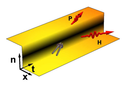 Figure 1
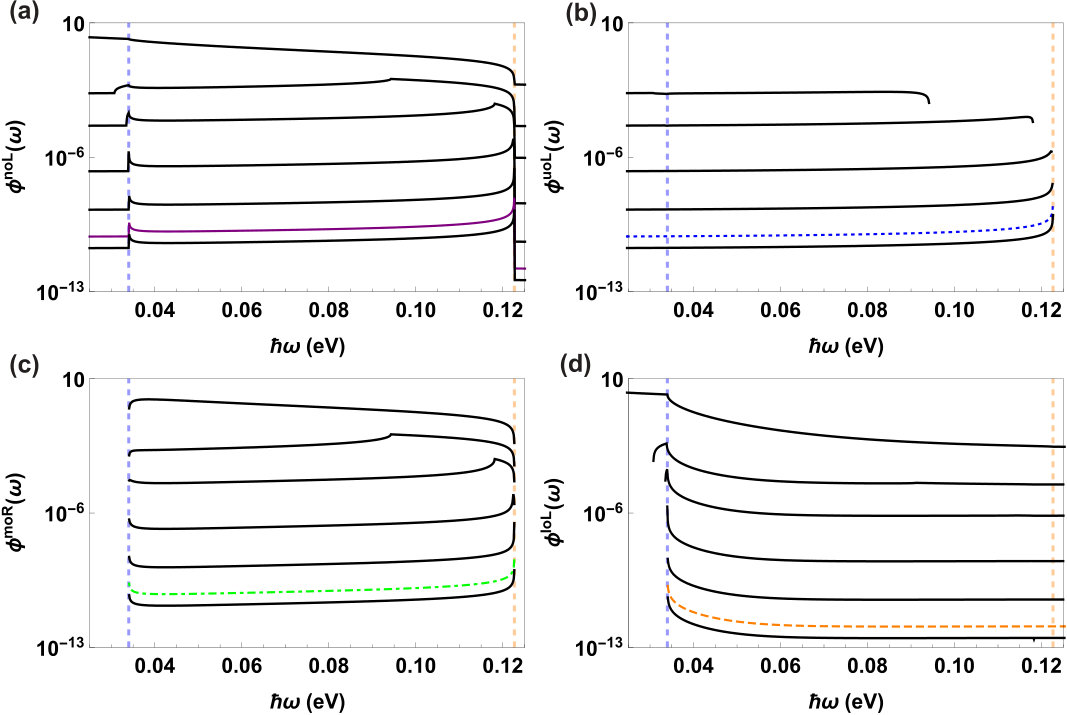 Figure 2
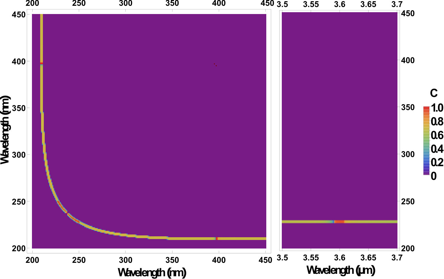 Figure 3
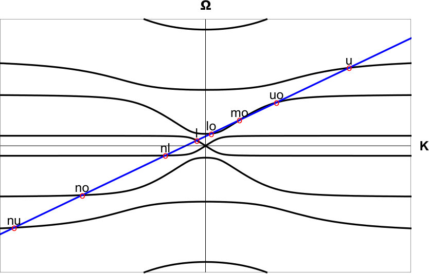 Figure 4
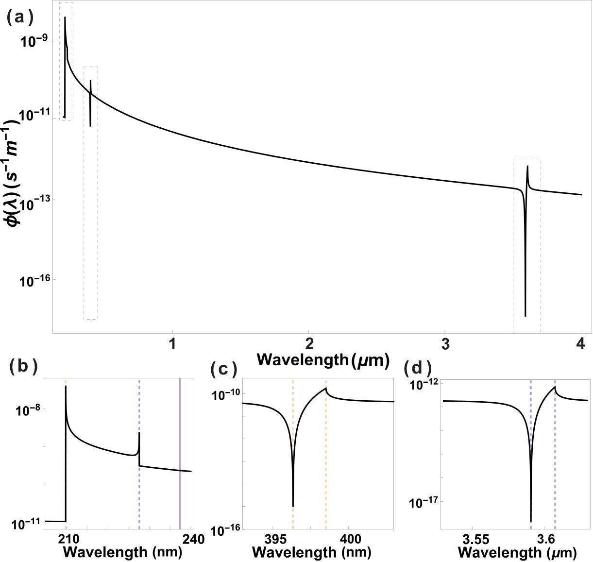 Figure 5
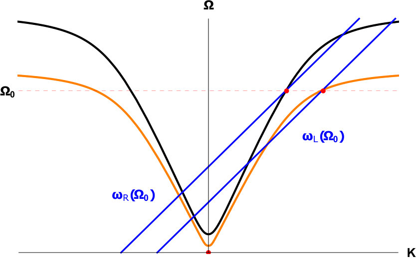 Figure 6
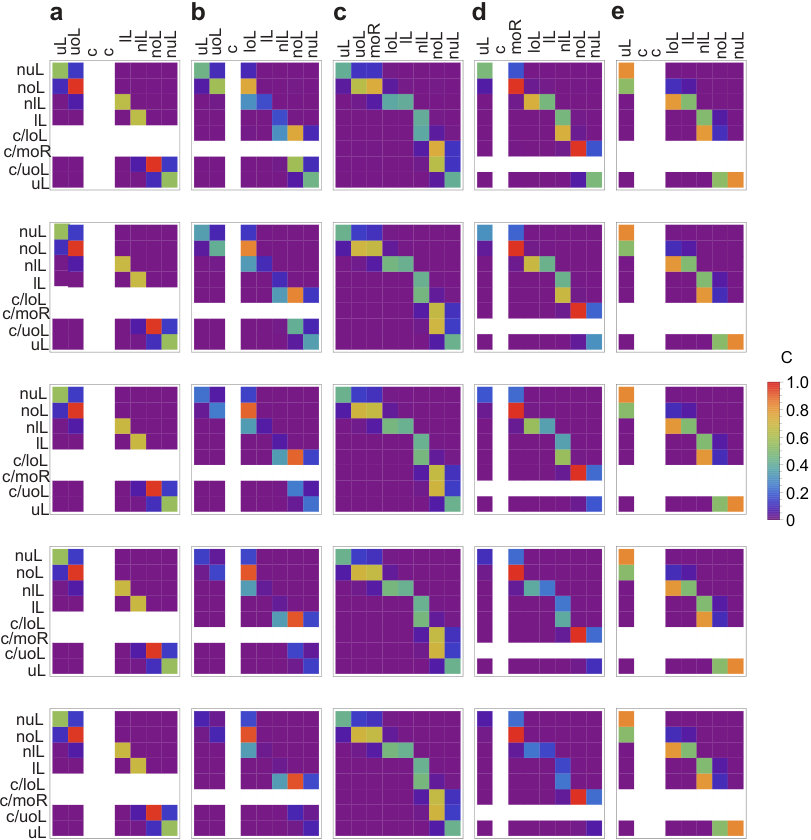 Figure 7
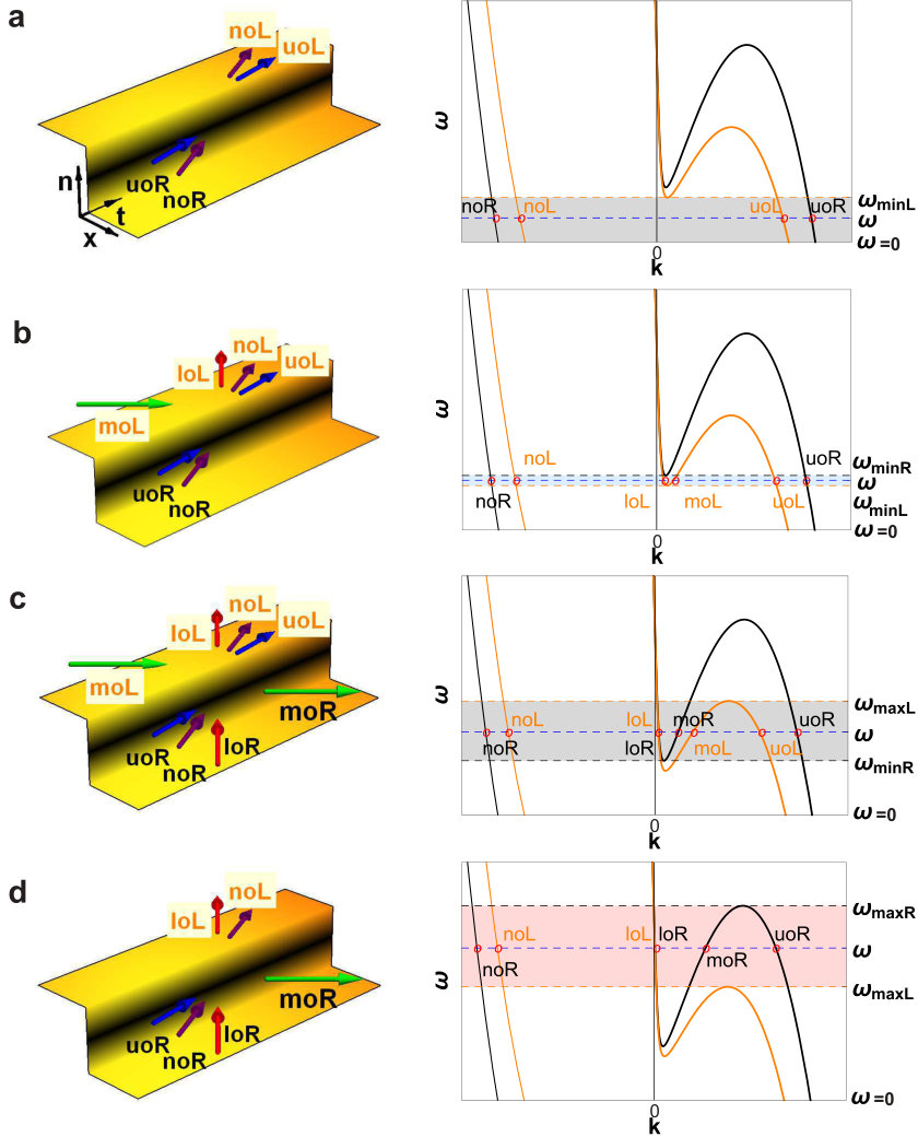 Figure 8
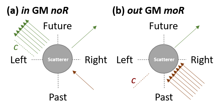 Figure 9
| RIF | White hole | Black hole | |||||||||
| (nm) | (nm) | (m) | C | (nm) | (nm) | C | |||||
|---|---|---|---|---|---|---|---|---|---|---|---|
Peer Reviews
No public reviews on file for this paper yet. If you reviewed it on a platform where reviews are public (OpenReview, ICLR, NeurIPS, ICML), you can paste yours below so the community can read it here.
Videos
No videos yet. Explain this paper in a talk, walkthrough, or lecture? Add one.
Analytical description of quantum emission in optical analogues to gravity
Maxime J Jacquet
Laboratoire Kastler Brossel, Sorbonne Université, CNRS, ENS-Université PSL, Collège de France, Paris 75005, France
Faculty of Physics, University of Vienna, Boltzmanngasse 5, Vienna A-1090, Austria.
Friedrich König
School of Physics and Astronomy, SUPA, University of St. Andrews, North Haugh, St. Andrews, KY16 9SS, United Kingdom
(16th March 2024)
Abstract
We consider a moving refractive index perturbation in an optical medium as an optical analogue to waves under the influence of gravity. We describe the dielectric medium by the Lagrangian of the Hopfield model. We supplement the field theory in curved spacetime for this model to solve the scattering problem for all modes and frequencies analytically. Because of dispersion, the kinematic scenario of the field modes may contain optical event horizons for some frequencies. We calculate the spectra of spontaneous emission in the frame co-moving with the perturbation and in the laboratory frame. We also calculate the spectrally-resolved photon number correlations in either frame. The emitted multimode field comes in different types depending on the presence of horizons. We show that these types are robust against changes in the system parameters and thus are genuine features of optical and non-optical analogues. These methods and findings pave the way to new observations of analogue gravity in dispersive systems.
††preprint: APS/123-QED
I Introduction
A number of classical and semi-classical features of gravity can be reproduced in the laboratory: it is possible to create effectively curved spacetimes for waves in media unruh_experimental_1981 and, in particular, event horizons. These horizons scatter waves and are predicted to spontaneously emit quanta by the Hawking effect hawking_black_1974 ; hawking_particle_1975 . Recently, experiments in many different ‘fluid’ systems, such as Bose-Einstein condensates lahav_realization_2010 ; munoz_de_nova_observation_2019 , water rousseaux_observation_2008 ; weinfurtner_measurement_2011 ; Rousseaux_PRL_2016 ; torres_rotational_2017 ; euve_wormholes_2017 ; euve_scattering_2020 and polariton microcavities nguyen_acoustic_2015 have demonstrated horizons and studied the behaviour of waves in their vicinity. New developments in quantum fluids of light michel_superfluid_2018 ; Fontaine_disprel_2018 ; jacquet_fluids_2020 may soon enable novel analogue gravity experiments.
As in the astrophysical case hawking_particle_1975 , the paired spontaneous emission in analogues results from mixing of field modes of positive and negative Klein-Gordon norm at the horizon unruh_experimental_1981 . Thus, pairs from horizons have been extensively studied for fluid systems, in which their nonseparability in various dispersive regimes has been investigated Busch_entanglementHR_2014 ; Busch_entanglementfluid_2014 ; finazzi_entangled_2014 ; boiron_quantum_2015 ; michel_phonon_2016 ; weinfurtner-BEC-HR-2016 , and are considered an unmistakable signature of the Hawking effect schutzhold-unruh-comment-2011 ; finke_observation_2016 ; fabbri_momentum_2018 ; coutant_low-frequency_2018-1 ; coutant_low-frequency_2018 ; isoard_quantum_2020 .
It is also possible to create effectively curved spacetimes for light in dispersive media. As an optical pulse moves through the dispersive medium, the pulse intensity locally raises the refractive index of the medium by the optical Kerr effect, creating a moving refractive index front (RIF). Light under the pulse is slowed by the increased index, i.e., light of some frequencies will be slowed below the pulse speed and captured into the RIF. This is in analogy with the kinematics of waves at a black-hole event horizon visser_acoustic_1998 ; leonhardt_laboratory_2002 ; schutzhold_EMW_2005 ; gorbach_light_2007 ; philbin_fiber-optical_2008 ; Hill_soliton-trapping_2009 ; faccio_analogue_2010 ; choudhary_efficient_2012 ; Jacquet_book_2018 ; drori_observation_2019 . At other frequencies, however, the kinematics of light waves are different Jacquet_quantum_2015 ; jacquet_influence_2020 , recreating wave motion at a white-hole event horizon or two-way motion towards and away from the RIF. Emission in all these kinematic scenarios occur simultaneously.
The RIF may be time independent in the moving frame: the system is stationary and can be described efficiently by the scattering matrix. Possible analytical methods to arrive at the scattering matrix broadly fall under two categories, depending on the profile of the RIF considered: for smooth RIFs belgiorno_hawking_2015 ; linder_derivation_2016 , the JWKB approximation is used to calculate the asymptotic states (far from the RIF) that are matched with the near-RIF expansion (which is instead treated in Fourier space), whereas no approximations are needed in the case of a step-like RIF finazzi_quantum_2013 . Although the step is physically hard to implement, because the particles are emitted from a single point, this simple optical system allows us to contrast the quantum emission in the different kinematic scenarios highlighted above. The output fields will be further modified by gradual horizons, two-horizon interactions and other nonlinear effects such as optical Čerenkov radiation. Studying the RIF allows us to identify which quantum effects are connected with a single horizon. The approach of finazzi_quantum_2013 needs to be comprehensively generalised to account for the possible change of kinematic scenarios, and to include a treatment of evanescent waves in these scenarios as well as a derivation of the full scattering matrix. From the scattering matrix follow the output quantum fields for all modes. In particular, we are interested in key output observables — such as photon-number spectra and correlations — which are of principal importance in any theoretical or experimental study of analogue gravity. The calculation of the photon-number correlations is challenging because it requires accounting for the dispersion and the bandwidth of the modes.
In this paper, we supplement and extend the theoretical description of the spontaneous emission at a step-like RIF of finazzi_quantum_2013 , as shown in Fig.1. We present an analytical method to calculate the scattering matrix in all kinematic scenarios in a dispersive dielectric featuring intra- and inter-branch scattering. Moreover, we demonstrate the calculation of key quantities measurable in the medium rest frame, viz. the photon emission spectral density and the spectrally-resolved photon-number correlations, as they are recorded with a variable bandwidth detector. We find pertinent features when modifying the parameters of the system.
In section II, we review all possible kinematic scenarios for waves at the RIF and explain their relevance in the anlogy with gravity. Section III derives the photon flux in different frames as well as the spectral correlations detected with variable bandwidth detectors in terms of the scattering matrix. Section IV derives the scattering matrix for all modes and frequencies from the field matching conditions at the RIF. In section V we use our method to compute observables in bulk fused silica. We calculate key observable quantities, namely the spectral density of spontaneous emission and the spectral correlations, in the rest frame of the medium and discuss their dependence on the RIF height and velocity. We also briefly discuss desired medium properties.
II Kinematic scenarios
Our study is based on the consideration of the step-like geometry of a RIF that propagates at constant speed in the positive -direction in the laboratory frame. This RIF is illustrated in Figure 1 in co-moving frame coordinates and . In Appendix A we review and supplement the field theory for light in an inhomogeneous dispersive dielectric. There we find the modes of the homogeneous medium and construct the ‘global modes’ (GMs) of the inhomogeneous system (including the step). Finally we quantise the field which is represented by annihilation and creation operators of the GMs. In this section, we review the kinematics of light waves at different frequencies Jacquet_quantum_2015 and explain the analogy with gravity.
The RIF separates two regions of homogeneous refractive index whose dispersion is modelled by (cf. App A)
[TABLE]
with and the frequency and wavenumber in the frame co-moving with the RIF at speed (). and are the medium resonant frequencies and elastic constants. The change in index, , at between the two regions, is modelled by a change in and in (1). As illustrated in the dispersion diagrams of Fig.2, the step manifests itself as a change in the dispersion relation between the low (, black curve) and high (, orange (light grey) curve) refractive index regions.
The two parts of the optical branch, shown in Fig.2 for frequencies of relevance, represent negative- (positive-) norm modes on the left (right) in the diagram. Modes are marked with open circles. For all , there is one negative-norm mode (thin) and, in addition, either one or three positive-norm modes (thick). We refer to frequency intervals of with three positive norm modes as subluminal intervals (SbLIs): and . Inside a SbLI, one of the four mode solutions has a positive group velocity in the moving frame, moving rightwards. We call this mode ‘mid-optical’ — ‘moL’ on the left, and ‘moR’ on the right of the boundary. Note that in no other mode may light propagate with positive group velocity. There is also the ‘low optical’ mode loL/R, the ‘upper optical’ mode uoL/R, and the ‘negative optical’ mode noL/R. Beyond the SbLIs, i.e. for or , only two propagating modes remain. Thus, in growing order of we find the following distinct kinematic scenarios at the step:
Fig.2 a. Two optical propagating modes (noL/R, uoL/R) are present, with negative group velocities in the moving frame on either side. Light in all modes may only move to the left. 2. -
Fig.2 b. On the left of the interface, four optical propagating modes are present (noL, loL, moL, uoL) whilst only two modes (noR, uoR) are present on the right. Mode moL has positive group velocity, whereas all other modes have negative group velocity. Light can propagate into the boundary from the left, but cannot proceed further to the right. The interface acts as a white hole horizon to light. 3. -
Fig.2 c. Four propagating modes (noL/R, loL/R, moL/R, uoL/R) exist on either side of the interface. Modes moL and moR have positive group velocity on the left and on the right of the RIF, respectively. The RIF is not a one-way door. 4. -
Fig.2 d. On the left of the interface, two propagating modes are present (noL, uoL), whilst four optical modes are present on the right (noR, loR, moR, uoR). Light on the right can move in either direction, but on the left of the interface both modes have negative group velocity. There is a one-way door from the right to the left: light experiences a black-hole horizon at the RIF.
For the largest , the kinematics return to the type of Fig.2 a.
Only in scenarios b and d is a subluminal region paired with a superluminal region, creating a horizon. This is in analogy to the superluminal space flow in the interior region of a black- or white hole and the subluminal flow outside jacquet_influence_2020 . The analogy to gravity is best understood when thinking of black hole emission by the Hawking effect: a positive norm mode — Hawking radiation — allows for energy to propagate away from the hole in the subluminal region, while its negative norm partner falls inside the horizon. The black hole kinematics as illustrated in Fig.1 are realised in Fig.2 d: mode moR allows for light to escape the horizon to the right, like Hawking radiation, and mode noL is the infalling partner.
This analysis of kinematic scenarios is interesting because it shows that optical analogues may allow us to access features of gravity physics other than wave motion at the event horizon of black holes. The simple geometry of a localised step allowed us to identify the above kinematic scenarios. A continuous RIF would also exhibit one of these four scenarios at any one point .
In all 4 kinematic scenarios, the motion of the RIF in the dispersive medium creates a non-adiabatic modification of the refractive index in time , which corresponds to a time-dependance of the spacetime curvature. Thus, modes (even in the vacuum state) will scatter at the RIF. We use the S-matrix formalism to describe this mode coupling.
III Analytical calculation of spectral densities and correlations
The aim of the field theory summarised in appendix A is to enable the calculation of all output properties in terms of the scattering matrix . In Jacquet_quantum_2015 , we calculated the output spectral density in all output modes. Paired production in these modes, which is at the heart of the Hawking effect, is best characterised by the photon number variances and covariances. Here, we derive these quantities for an optical system for the first time.
In appendix A.2 we construct two basis sets of global modes (GMs) of the system: the in and out bases. We calculate the spontaneous emission in out modes, i.e., the in modes are in the vacuum state . Because the system is in a stationary state, the photon flux for an out mode is given by the integral over the frequency correlation loudon_2000 :
[TABLE]
The flux is the dimensionless number of photons per unit time and unit bandwidth at in the moving frame. We now replace the out-mode operators in the frequency correlations using the scattering transformation (41) by in-operators, which act directly on the in vacuum state. Using the frequency correlation (E) calculated in appendix E, we express the photon flux by the -matrix
[TABLE]
is the set of modes which have a positive (negative) norm if is of positive (negative) norm. The photon flux results from the scattering of in modes into out modes of opposite sign of norm. The number of emitted photons depends solely on the scattering matrix , bandwidth and interaction time.
The total photon number is obtained by integrating over all frequencies and time. To obtain the photon number over a limited ‘detected’ frequency interval in this stationary mode conversion process, the field operators have to be constrained to this bandwidth. This is achieved via the spectral filter function , which takes the value of 1 if the frequency is in the detected interval and 0 otherwise. Then
[TABLE]
is the interaction time in the moving frame. From (4), one may calculate other important quantities, such as (3) and the photon-number correlations across the spectrum.
Correlations in photon number between modes and are found by calculating the normally ordered covariance of the photon numbers and on detectors 1 and 2:
[TABLE]
In (5) the expectation value is again taken with respect to the in vacuum state and and are the filters for detectors 1 and 2, respectively. This defines the spectral intervals and over which these detectors collect photons. We calculate the fourth order moment of the field in Appendix E. Inserting the result (73) into (5) we find
[TABLE]
Here is identical (complex conjugate) to if mode is of positive (negative) norm. equals unity if the correlated modes and have identical (opposite) norm and zero otherwise. Reverting from back to , we observe that in the -term two elements have to be conjugated and in the -term either all or none. Since the result, as well as , are real, the first two sums in (6) are equal. Hence we observe that the mutually exclusive and exhaustive and let us combine the first two terms into one and the last two terms cancel due to (41), (3) and (4):
[TABLE]
is the spectral overlap (moving frame frequencies) of the two spectral intervals and of the two detectors. This result allows us to quantify the spectrally resolved photon number correlations of any stationary process in quantum optics. The correlations are contained in the scattering matrix and are dependent on the spectral overlap of the detectors regarding the investigated mode.
We also calculate the variance . Using the not normally ordered moment derived in (74) of App. E in a not normally ordered expression equivalent to (5), and with , we obtain
[TABLE]
The photon-flux Pearson correlation coefficient between detectors 1 and 2, corresponding to modes and . It is
[TABLE]
In the last step we have assumed the scattering matrix to change little across a narrow detection bandwidth. The normalisation ensures that . Note that this also means that C is independent of the photon flux. The correlations generated by the scattering are entirely positive, indicating their origin of entangled photon pair generation from the vacuum. From (9), we can easily extract the (narrow bandwidth) self-correlation with matched filters
[TABLE]
which is a measure of the noise in mode relative to the Poisson noise variance of . Using (8), we see that C increases from 0 (vacuum) and approaches 1 (maximum noise) for increasing photon numbers.
Furthermore, we calculate the second order correlation function . Again assuming narrowband detection, we obtain:
[TABLE]
as well as the single detector correlation
[TABLE]
Here we recover the expected result that the scattering induces correlated noise between the two detectors, both of which detect the statistics of chaotic light. These relations describe output observables in any process described by the scattering matrix but are particularly tailored to analogue gravity in dispersive systems, in which context they appear for the first time.
The photon numbers and correlations up to this point are calculated in the moving frame where the system is stationary. However, in an experiment, measurements are performed in the laboratory frame, so we now proceed to derive the flux there. Photon numbers and time-bandwidth products are frame invariant. Therefore, re-interpreting and as the laboratory interaction time and detection bandwidth, the laboratory frame correlation coefficient of modes and is identical to Eq.(9). All other relations containing photon number operators can be interpreted for the laboratory frame as well.
For light waves to reach the detector, the out global modes (GMs) must have a positive laboratory-frame group velocity. As can be seen in Fig.8, modes no and uo have positive group velocities. So too does mode lo, except if is negative (at very large ). These modes are the out GMs on the left. In the low-index region on the right, the only out GM, i.e., propagating away from the RIF and ahead of it, is mode moR. Thus, when calculating the laboratory frame spectral density at optical frequencies, we expect to detect contributions from the out GMs loL (at low ), moR, uoL and noL.
The moving frame flux density in out GM is (3). The laboratory frame flux density is obtained from this by finazzi_quantum_2013
[TABLE]
The total spectral density at , , is found by adding contributions of all GMs:
[TABLE]
Here, we have to consider that a laboratory-frame detector might detect more than a single mode . Assuming the detector is sensitive to a frequency , then we can read off the laboratory frame dispersion diagram (Fig.3) that there are two modes with and opposite . Note that there is another pair of solutions at . Out of the four solutions exactly one has positive group velocity and positive moving frame frequency . Thus the detector frequency corresponds to a unique mode in general, although we remark that two exceptions are possible: (a) The detected frequency interval could contain the boundary frequency separating two modes, e.g. moR and uoL. In this case the interval is reduced to the detected mode with group velocity away from the RIF. (b) Two out-GMs from either side of the RIF might share a laboratory frequency (Fig.3). In this case they typically do not share the same moving frame frequency () and the covariances and variances of the modes add up, as for incoherent fields.
The wavelength equivalent to (14) is
[TABLE]
with ; the laboratory frame wavenumber; the modes that contribute to the emission at , and their moving frame flux density (3); the mode’s group velocity in the laboratory frame.
Equation (15) completes this section, where we formulated the important output observables for optical analogue gravity in both frames. These quantities are the tools we will use in section V to characterise and typify the emitted field in the moving and laboratory frames.
IV Analytical calculation of the scattering matrix
As we have seen in the previous section, the quantum field for all modes explicitly follows from the scattering matrix, and we now build on the field theory of appendix A to derive the latter analytically for the first time. We calculate the scattering matrix at all frequencies (from all kinematic scenarios) and include evanescent waves in the calculation, and thus our method lends itself to considerations of more general RIF profiles.
We continue to use the step in the index, as in Fig.1. For a monochromatic field of frequency , the canonical conjugate momenta and as well as their first spatial derivatives can be expressed by the electromagnetic potential , the polarisation fields as well as their derivatives in a homogeneous region using (25), (26) and (28) (App. A). Therefore the field vector can be reexpressed by the vector . The prime denotes the spatial derivative of the field. will allow us to simplify the matching conditions below.
and are related by Eqs.(25)-(28) as:
[TABLE]
for a field at frequency . We call the matrix in (16) , and note that . We make (16) applicable for global modes by defining . We may combine eight plane wave modes () into a mode set as a matrix
[TABLE]
with ’s ordered by laboratory-frame frequency. L/R corresponds to a basis set of local modes on either side of the boundary at . This is similar to (37).
In order to describe the mode coupling at the RIF with the scattering matrix formalism, we construct the global modes (GMs) of the inhomogeneous system, introduced in section A.2 of App. A. These GMs are linear combinations of the plane wave solutions , the local modes (LMs), for each homogeneous medium on either side of the RIF. There are complete sets of global in modes,
[TABLE]
and global out modes,
[TABLE]
Each global in (out) mode contains only one LM, whose energy flux is directed into (out of) the boundary. Because there are LMs connected at the index boundary, there exist 16 GMs: 8 in and 8 out. In (18) and (19), each -matrix contains the coefficients of the 8 local modes for the 8 global modes.
The mode decompositions of GMs into LMs on the left and on the right of the interface, respectively, are related by the matching conditions at the interface. For in and out modes at , we write
[TABLE]
This leaves us with 64 unknowns in either (20) or (21). The ’s are known, so we can obtain all ’s (we calculate an example in Appendix C). We calculate the scattering matrix by relating the in and out GMs as:
[TABLE]
Insertion of (18) and (19) into (22) yields :
[TABLE]
Now we have demonstrated how to completely characterize the scattering off a RIF analytically by calculation of the scattering matrix. In Appendix C, we exemplify one mode configuration in detail (further calculations can be found in Jacquet_book_2018 ), and explicitly derive the in and out matrices, and the corresponding scattering matrix. In Appendix D, we show that the scattering matrix is quasi-unitary, and thus correctly normalised.
V Spectra of spontaneous emission
We now put the analytical formulas developed in sections II-IV into action to exemplify their use, and more importantly to study our dispersive, multimode system. The system is reduced to the essentials of analogue horizon physics, compared to more comprehensive and realistic systems.
We calculate the scattering matrix and compute 1- and 2-photon spectra of spontaneous emission. Optical analogue experiments are different from their fluid-based counterparts (such as BECs munoz_de_nova_observation_2019 , water waves rousseaux_observation_2008 ; weinfurtner_measurement_2011 ; Rousseaux_PRL_2016 or fluids of light nguyen_acoustic_2015 ; Fontaine_disprel_2018 ; michel_superfluid_2018 ; jacquet_fluids_2020 ) in that the reference frames are exchanged: the rest frame of the optical experiment corresponds to the frame of the moving fluid, and vice versa. In both analogues, the measurements are performed in the laboratory frame. Here, we present spectra and mode-correlation maps in both frames to predict observations in optics and to allow comparison to fluid-based analogues.
We continue with the example of light in bulk fused silica at a step-like RIF as in section II. The Sellmeier coefficients in (1) are: , , and for the elastic constants, and , , and for the resonance frequencies Agrawal_2012 . Here, we present computations for various step heights, from to . We first consider a RIF moving at velocity in bulk fused silica and later vary the velocity of the RIF (in section V.3).
´
V.1 Moving frame spectra
In the moving frame, the contributions of the different modes under the various kinematic scenarios are most apparent. We use the formulas developed in sections II-IV to calculate 1- and 2-photon spectra. We also investigate the influence of the step height, which we change over a (realistic) range of 5 orders of magnitude, on the emission.
We start by computing the spontaneous photon flux (3) in the moving frame in the four optical modes, see Fig.4 ((a) noL, (b) uoL, (c) moR and (d) loL) for various step heights . The emission in all modes increases with step height. The frequency intervals with horizons are located at the blue and orange dashed lines for the white hole interval (WHI) and black hole interval (BHI), respectively (kinematic scenario of Fig.2 b and d). Except for the three highest step heights, the frequency intervals with event horizons are very narrow (e.g. 1 and 10 eV for the WHI and BHI, respectively, at ). Here we observe the following emission peaks: modes loL and noL both form a peak at the WHI, whereas modes moR and noL both form a peak at the BHI. Otherwise, modes moR and uoL sharply increase towards the WHI and BHI, respectively, but neither of them exists there. Outside the horizon intervals the emission is spectrally wide and smooth. We observe that horizons increase the emission.
Spectra in the horizon intervals assume the shape of a shark fin, best seen at higher step heights (, ) as the horizon intervals widen for emission into mode noL at the WHI and BHI (a), mode moR at the BHI (c) and mode loL at the WHI (d). This shape is created because on one side (large and small ) the emission cuts off by orders of magnitude as an emitting mode (moR and loL) ceases to exist outside the interval. On the other side, the horizon condition cuts off because we approach the kinematic scenario of Fig.2 c, leading to an abrupt decrease in emission. At the highest step height the BHI expands and the WHI disappears, leading to a more uniform emission. The shape of the spectrum is formed by the change in kinematic scenario Jacquet_quantum_2015 .
Spontaneous emission occurs in pairs of photons, so we expect the photon number in any mode to be correlated with that in (at least) one other mode. Partnered emission can be characterised further by computing the matrix of mutual photon number correlations between all modes. Fig.5 shows the photon-flux correlation coefficient (9) of two modes at typifying frequencies and for . Correlations (e.g. top row) are generally strongest between the optical modes. Because noL is the unique negative-norm optical mode, we find the strongest correlation between this mode and positive-norm optical modes. We observe that the correlations are different if horizons exist (Fig.5 columns b, d). Over the WHI (BHI), there is a single large correlation between noL and loL (noL and moR), with other correlations being small or zero. In both cases, the pairs of modes correspond to the Hawking radiation and the partner. Importantly, partnered emission does not occur solely in the frequency intervals where the kinematics are analogous to the curvature of spacetime at a black- or white-hole horizon, but occurs in the other kinematic scenarios as well. Without horizons (Fig.5 a, c, e), significant correlations exist between typically three mode pairs simultaneously, indicating multipartite entanglement. These involve non-optical modes, although the flux is weak Note1 . As can be seen by comparing the columns of Fig.5, the magnitude of the correlation coefficients as well as their structure are surprisingly independent from the step height, although this varies over 5 orders of magnitude.
To summarise, the flux of spontaneous emission is dominated by white- or black hole-horizon physics and drops significantly beyond that. The spectral characteristic is a ‘shark fin’ shape. Over the analogue white- and black hole intervals, paired two-mode emission at optical frequencies dominates. These observations are robust over a wide range of step heights .
V.2 Laboratory frame spectra
Using our formulas for observables further, we now compute laboratory frame spectra and identify the signature effects as observed in the laboratory frame. Because we have found the signatures of horizon physics to be robust against changes in the step height , we now limit our discussion to .
The laboratory frame spectrum (15) is computed in Fig.6. Similar to its moving frame counterpart, it consists of intervals of white hole, black hole and horizonless emission. Emission is sharply peaked over analogue white- and black-hole intervals, and dips down at wavelengths which are velocity-matched with the RIF. These features are therefore ruled by the kinematic scenarios explored in Fig.2. The peak at () nm corresponds to black- (white-) hole emission into the optical negative-norm mode (noL). From there, the spectral density decreases towards nm. At nm, mode uoL is velocity-matched to the RIF, becomes complex, and the emission drops. The drop is limited to 5 orders of magnitude because at nm black hole emission into mode moR cuts on. Finally, we observe peaks at nm and around m that account for the black hole and white hole emission into positive norm modes moR and loL, respectively. Note that, whereas in the moving frame the frequency sets the kinematic scenario, in the laboratory frame the spectral density may emerge from different scenarios. All peaks in Fig.6 (b), (c) and (d) exhibit the signature ‘shark fin’ structure of horizon emission. Clearly, these are signature effects of horizon physics in dispersive (optical) media.
The various spectral peaks and dips we have identified have narrow linewidths: about nm below nm, nm around nm and nm at m. They are expected to have strong spectral correlations.
Fig.7 presents the photon number-correlation coefficient (9) across the spectrum of laboratory frame emission. Measuring these photon-number correlations convincingly reveals their vacuum fluctuations origin. Coefficients between different modes display a single continuous contour of significant photon number correlations across the entire spectrum. The contour indicates correlations between the negative-norm mode noL (below nm) and the positive-norm modes uoL (between nm and nm) or moR (beyond nm). The contour thus indicates where these mode pairs share a common moving frame frequency . Note that this depends on dispersion in a nontrivial way and is not a hyperbolic relation. The correlation coefficients of Fig.5 and Fig.7 are mostly identical for identical frequencies . Along the contour in Fig.7, starting at mn, the correlation coefficients gradually decrease as the wavelength of noL decreases and the wavelength of mode uoL, and subsequently of mode moR, increases, up to a point around ()(nm, nm) where the black hole horizon is formed and the correlation coefficient suddenly peaks. We observe the strongest coefficient, , at (nm, nm) — between modes moR and noL. Partnered emission also dominates over the WHI (m, nm) with — between modes loL and noL. In both cases, the coefficients mainly deviate from unity because of weak correlations with non-optical modes ( and ). The quantum state is almost a pure two-mode squeezed vacuum jacquet_influence_2020 . The strong correlation between outgoing modes only if separated by a horizon is characteristic of the Hawking effect. On the diagonal, the self-coefficients (10) characterize the photon number noise relative to Poisson noise. These elements are very small as individual modes carry chaotic noise and the photon numbers are small.
V.3 Robustness of the spectra against changes in dispersion
Finally, we discuss the experimental implementation of this optical gravity analogue via the prism of the detection of Hawking radiation (HR). The RIF might be generated by an optical pulse via the optical Kerr effect. The velocity then corresponds to the group velocity of that pulse. Changing by way of dispersion, e.g. by shifting the pulse frequency, will therefore alter the wavelengths of the black- and white hole emission: these are found close to wavelengths which have the same group velocity as the RIF.
In Table 1 we show the laboratory-frame properties (wavelength, spectral density and spectral correlations) of white-hole and black-hole emission for four pulse group velocities (or wavelength ): ( nm), ( nm), ( nm) and ( nm). While nm is the zero dispersion wavelength, where the group index assumes a maximum, nm and nm share the same group velocity. The table shows that overall emission wavelengths for the optical modes are shifted, but the correlation strengths are largely robust. The flux strength changes moderately with the pulse velocity. However, because the black hole emission into mode moR is very close to the pulse wavelength, it will be difficult to distinguish it from photons of the pulse. Also, the white hole emission at infrared wavelengths is hard to detect.
When the group velocity of the RIF matches the group velocity of waves in the visible, the Hawking effect may create pairs of photons in the UV (the partner) and visible (HR). This can be achieved by using a similar medium to ours, for example metamaterial waveguides, such as photonic crystal fibres philbin_fiber-optical_2008 ; choudhary_efficient_2012 ; Jacquet_book_2018 ; mclenaghan_compression_2014 ; drori_observation_2019 . In the anomalous dispersion region, a soliton can be generated in the fibre Agrawal_2012 . In this case, wavelengths in the visible/UV range might be velocity matched with the pulse: the emission from the front or back of the pulse will be found in this range, where the pulse edge constitutes a horizon. Other nonlinear effects such as the Raman effect, phase-matched four-wave mixing or Čerenkov radiation may take place in the medium but may be distinguished by their respective spectral signature.
VI Conclusion
We considered the mixing of modes of positive- and negative-norm in various kinematic scenarios in dispersive optical analogues to gravity. The refractive index front (RIF) may act as a black- or white hole horizon or as a horizonless emitter simultaneously. We presented a theoretical model (expanding on the canonical adaptation schutzhold_dielectricbh_2002 ; finazzi_quantum_2013 of the Hopfield model hopfield_theory_1958 ), formulated observables in the relevant reference frames and calculated the two-particle spectrum of an optical analogue for the first time.
We obtained a broad and structured spectrum with emission peaks in pairs of modes. The emission is in entangled photon pairs and occurs strongly from horizons on a background of a broadband, weak and horizonless emission. We change the height of the RIF over 5 orders of magnitude, and find that the signatures of horizon emission are not affected: the quantum correlation structure remains intact and the emission shape does not change.
These effects are largely robust against changes in dispersion as well, and we identify nonlinear waveguides as media of choice to observe horizon physics. The resulting spectral peak, spectral correlations and their dependence on RIF velocity and medium dispersion are key identifiers of the type of spontaneous emission at the horizon by the Hawking effect or the horizonless emission.
This analytical method can be generalised to study other RIF profiles, such as a finite-length pulse, and to calculate the spectra and their spectral correlations. This is essential to identify the optimal conditions to observe the Hawking effect. Importantly, the method can be used to provide a theory trace for optical analogue experiments, to learn more about the Hawking effect, and to study a variety of effects such as cosmological pair creation by passing gravitational waves or expanding/contracting universes weinfurtner_cosmological_2009 ; eckel_expanding_2018 ; campo_inflationary_2005 ; campo_inflationary_2005-1 ; campo_inflationary_2006 , the so-called black hole laser gaona-reyes_laser_2017 ; bermudez_resonant_2019 , analogue wormholes, and the quasi-bound states of black holes patrick_black_2018 .
Acknowledgements.
The authors are thankful to Bill Unruh, Joseph Cousins, Stephen Barnett, Vyome Singh and David Bermudez for insightful conversations. This work was funded by the EPSRC via Grant No. EP/L505079/1 and the IMPP.
Appendix A Field Theory
A.1 Light in an inhomogeneous dispersive dielectric
Following schutzhold_dielectricbh_2002 ; macher_black/white_2009 ; finazzi_quantum_2013 and Jacquet_quantum_2015 , we describe the interactions of light with an inhomogeneous and transparent dielectric by a microscopic model based on the Hopfield model hopfield_theory_1958 . We consider one-dimensional scalar electromagnetic fields and operate at frequencies sufficiently far from the medium resonances to neglect absorption. The medium consists of polarisable molecules — oscillators with eigenfrequencies (resonant frequency) and elastic constants . Since the wavelength of light is large compared to the molecular scale, we consider the dielectric in the continuum limit and describe the electric dipole displacement by the massive scalar field . The electromagnetic field (a massless scalar field) is described by , the -component of the vector potential (with in temporal gauge), where and are space and time in the laboratory frame.
Our study is based on the consideration of the step-like geometry of a RIF, that propagates at constant speed in the positive -direction in the laboratory frame. The RIF is shown schematically in Fig.1 in the co-moving Lorentz frame coordinates and . We locate the boundary of the RIF at . We focus entirely on the index change induced by the RIF, neglecting phonon interactions and phase-matched optical nonlinearities such as four-wave mixing. In both homogeneous regions (), the interaction of the electromagnetic field with the three polarization fields of the medium is described by the Lagrangian density finazzi_quantum_2013 ; Jacquet_quantum_2015 ; hopfield_theory_1958
[TABLE]
where is the inertia of oscillator and . Most transparent dielectrics are sufficiently well described by three resonances and so we use . The term linear in in Eq.(24) describes the coupling between the fields. The Lagrangian density accounts for the free space and medium contributions to the field through the first two terms and the sum, respectively. Dispersion enters as a time dependence of the addends of the summation.
By the principle of least action, we obtain the Hamiltonian density by varying the Lagrangian density (24) with respect to the canonical momentum densities of light and the polarisation fields. From the Hamiltonian density follow the Hamilton equations, the equations of motion for the fields finazzi_quantum_2013 ; cohen-tannoudji_photons_2004 :
[TABLE]
where the derivatives are with respect to and ’s denote the fields canonical conjugate to and . We go to Fourier space by and , where and are, respectively, the wavenumber and frequency in the moving frame. We obtain the generic Sellmeier dispersion relation of bulk transparent dielectrics Sellmeier_1871 , Eq.(1) of the main text:
[TABLE]
We complexify the massive field obtained from the action of (24) by identifying harmonic plane wave solutions to (25)-(28) of the form
[TABLE]
where is the eight-dimensional field vector . We can denote a single frequency field vector as , where indicates a particular solution of (29) for , i.e., a ‘mode’.
By construction, the Lagrangian (24) is invariant under global phase shifts of the dynamic fields. This continuous symmetry implies a conserved Noether current Jacquet_book_2018 ; cohen-tannoudji_photons_2004 . As a result, the Klein-Gordon product
[TABLE]
is conserved, and so is the induced norm . Here is the identity matrix and the Planck constant prefactor was inserted for normalisation. It can be shown that the Klein-Gordon norm of a positive (negative) laboratory frequency field is also positive (negative) finazzi_quantum_2013 ; rubino_negative-frequency_2012 ; mclenaghan_compression_2014 . As a result, waves of positive frequency in the moving frame can have either sign of the norm. This is different from fluid systems, where the sign of the norm is equal to that of the wave number . In optical systems, the Hawking effect takes place in correlated photons of positive and negative frequency , not wavenumber.
We orthonormalise a set of single mode field vectors () using the condition finazzi_quantum_2013 :
[TABLE]
Here is the sign function that determines whether the mode has positive or negative norm. Moreover, by Lorentz transform and .
We now turn to the non-uniform medium, which consists of two homogeneous regions separated by a RIF. The index in each homogeneous region is described by the dispersion relation (29), with dispersion parameters () and () in the right (left) region. The index distribution in the moving frame is:
[TABLE]
is the Heaviside step function and () is the index on the right (left) side. In an extension of the oscillator model by P. Drude and H. A. Lorentz, parametrises the change of dispersion constants that leads to the index change schubert_nonlinear_1986 ; Jacquet_book_2018 :
[TABLE]
For small index changes it follows from (29) that .
Harmonic wave solutions of frequency have a propagation constant given by Eq.(29), which is an eighth order polynomial, and thus eight wavenumbers form the modes of the field with degenerate energy , as shown in Fig.8. On either side of the RIF, there are either eight propagating modes or six propagating modes and two exponentially growing and decaying modes, respectively, characterized by complex and . The solution space is eight dimensional and we can build a full set of solutions for that space. Modes can move towards and away from the RIF.
A.2 Global modes of the system
In section II, we have discussed all possible mode scenarios Jacquet_book_2018 . We proceed to construct modes of the inhomogeneous system, the global modes (GMs). These are solutions to the equation of motion that are valid in both regions. Global modes correspond to waves scattering at the RIF, and they describe the conversion of an incoming field to scattered fields in both regions. The GMs are superpositions of the plane wave solutions in the two homogeneous regions on either side of the RIF.
We connect the plane wave solutions , the local modes (LMs), for the homogeneous medium at the index boundary at . We show in Appendix B, that the field is continuous at the boundary. The derivative of the field in space and time is also continuous, except for . We refer to these relations as the ‘matching conditions’.
We construct GMs as
[TABLE]
where () are coefficients of the eight modes on the left (right) side of the RIF. Because the fields and their conjugate momenta are related, half of the 16 coefficients in (35) are constrained by the matching conditions, leaving eight independent global modes.
Usually, the GMs are constructed as follows: a particular GM is constructed from a LM with its group velocity either towards (in) or away from (out) the RIF macher_black/white_2009 , irrespective of whether the LM is on the right or on the left. A GM that emerges from a defining in LM forms a global in mode , see e.g. Fig.9 a. out LMs define global out modes . However, in order to accommodate for the unphysical modes, the procedure needs to be amended in the following way: if, on either side of the RIF, two modes are complex, they will have complex conjugate wave numbers and frequencies. These are non-propagating solutions without group velocities and cannot be normalised. In this case, the unbounded LM will define an unphysical GM, without other LMs on that side, which serves doubly as in as well as out mode. This procedure always defines eight in and out GMs. The LMs are complete solutions in the homogeneous regions, i.e., the sets and are two basis sets of the inhomogeneous medium. Let us consider the example of the black hole-like case (mode scenario d in section II). There is a unique out GM, mode moR, that allows for light to propagate away from the interface into the low index region. Its mode decomposition is shown in a spacetime diagram in Fig.9 b: it is a linear combination of 7 oscillatory LMs, in the right region, that have negative group-velocity, a non-oscillatory (i.e., with complex wavenumber) LM on the left and a unique mode that has positive group-velocity in the right region.
A.3 Quantum field theory of scattering at the RIF
Each in GM describes the scattering of a harmonic wave to various outgoing harmonic waves. Conversely, each out GM describes a single harmonic wave resulting from the scattering of various incoming waves. The scattering can be described in the in as well as the out basis. The transformation between the two bases defines the scattering matrix, or matrix:
[TABLE]
Forming a matrix () from the in (out) basis set, we describe the basis change as:
[TABLE]
The spontaneous photon creation occurs because the quantum vacuum is basis dependent. Hence the spontaneous emission and all mode conversion follows from . We proceed with the canonical quantisation formalism introduced in hopfield_theory_1958 , developed in the 1990s in huttner_canonical_1991 ; huttner_dispersion_1992 ; matloob_electromagnetic_1995 ; barnett_spontaneous_1992 ; barnett_quantum_1995 ; santos_electromagnetic-field_1995 , and used in schutzhold_dielectricbh_2002 ; finazzi_quantum_2013 ; finazzi_spontaneous_2014 ; belgiorno_hawking_2015 and Jacquet_quantum_2015 ; Jacquet_book_2018 for the global modes. We postulate the equivalent of the standard equal-time commutation relations on the fields and :
[TABLE]
[TABLE]
We expand the quantised global field in the basis of global in modes:
[TABLE]
where P (N) denotes the set of all positive (negative) norm global modes (unphysical modes can be associated with positive norm here). The expansion (40) for in (and its counterpart for out modes) defines the annihilation operators and the creation operators for each global mode , as well as the transformation between in and out creation and annihilation operators. Hence, let be the column vector containing all the annihilation and creation operators for positive- and negative-norm global in modes, respectively, and the corresponding vector for the out modes. Then the transformation of operators follows from (36) and (40) as:
[TABLE]
With the scalar product (31) and the mode expansion (40) we can derive explicit expressions for the annihilation and creation operators and show that their commutator is:
[TABLE]
where the first is the Kronecker-delta. This relation holds for in and out operators. The commutator confirms that the global modes defined here are independent Bosonic modes in a continuous multimode field.
Appendix B Matching conditions of the fields at the RIF
Here we derive the continuity of the fields across the RIF. On physical grounds, we consider the field, polarisation field, all conjugate momenta and their time derivatives to be finite. By construction of the model schubert_nonlinear_1986 , the elastic constant is discontinuous and the inertia of the polarisation fields is continuous at the interface between the two homogeneous regions (cf. (34)). For fields of single frequency the field’s time derivatives do not alter the spatial continuity of the fields. In the near-interface region, we integrate the equations of motion over space. We begin with (27):
[TABLE]
All finite terms integrate to zero in the limits and so
[TABLE]
Thus is finite and the vector potential is continuously differentiable at : and . Proceeding similarly with (26) leads to
[TABLE]
i.e. the polarisation fields are continuous at . Analogously we find from (28) that the conjugate momenta ’s are continuous. We established now the continuity of , , , and in (26), and so , too, is continuous: . Finally, turning back to (28), in which and are continuous, we see that discontinuity of implies discontinuity of . Subtracting the rhs of (28) on either side of the RIF at we obtain:
[TABLE]
Appendix C Scattering matrix from the matching conditions
We explicitly derive the scattering matrix for the mode scenario of Fig.1 c. This corresponds to a frequency with 8 propagating modes on either side of the RIF interface. We use (20) to obtain all ’s (or (21) for ’s) from a single matrix
[TABLE]
Combining (20) and (47) we relate the ’s on either side of the RIF. Each column of contains the coefficients of individual local modes to one of the global modes on that side of the RIF. We arrange the global and local modes, respectively, in decreasing order of , i.e. first , then and so on. We use the construction of GMs described above eq.(47), with the modes ordered as , and hence (20) writes:
[TABLE]
There are 64 unknowns, ‘empty’ components of the matrices. We obtain:
[TABLE]
For the out modes, (20) is
[TABLE]
and by comparison with (48) we exchange L R and replace by in (55) and (62). Furthermore, we invert :
[TABLE]
Finally, by (23), we obtain the scattering matrix
[TABLE]
In (65), we have completed the derivation of the matrix for mode scenario c with 8 propagating modes on either side of the interface. The coefficients are taken from (47), viz. from the normalized local mode components. This derivation follows on from the matching conditions for the fields and their first spatial derivative at the interface and results in a straightforward expression for that can easily be evaluated on a computer.
Appendix D Quasi-unitarity of the scattering matrix
The scattering matrix describes the basis change between in and out global modes. Both are orthonormal bases, at least when there are 8 propagating modes. In order to preserve orthonormality, the scattering matrix is constrained. Alternatively, this can be seen as the preservation of the commutator relation for in and out annihilation and creation operators.
The orthonormality of the in GMs and is defined by a matrix ,
[TABLE]
with respect to the scalar product (31). The only non-zero elements of are +1 or -1 on the diagonal, indicating the positivity or negativity of the mode norm. In the out basis we have the same number of negative modes, because the norm is conserved during scattering, and so relation (66) is also valid for out GMs, if we order the modes accordingly. Using (37) we calculate
[TABLE]
This relation is called ‘quasi-unitarity’ and means that (and ) is a member of the indefinite unitary group . We can reformulate this condition as a normalization condition for the rows (and columns) of as:
[TABLE]
where indicates the frequency sign and thus the norm of mode . Ensuring that the scattering matrix is quasi-unitary is a useful test for numerical implementations. The procedure is easily generalised for other cases, where there are complex, non-propagating mode solutions. As these generate non-physical modes, the scattering matrix becomes a block matrix and, although not normalizable, the norm of the unphysical mode can be defined as unity in .
Appendix E Higher order correlation function
Here we detail the calculation of photon number variances and covariances. These are expressed by the expectation value of the second and fourth order moments of the out annihilation operators, which we calculate here. The expectation value is taken with respect to the in vacuum state. Therefore, we write out the Bogoljubov transformation (41) Bogoljubov_1958 , which connects in and out operators, in the norm-independent way:
[TABLE]
where again stands for the set of modes with norm identical to . The matrix is equal to the scattering matrix except for the rows which belong to negative norm modes, that are complex conjugated. Creation operators for the out modes are then obtained by Hermitian conjugation of (69) only. Note that this expression is valid for any mode , whether of positive or negative norm.
We start with the second moment
[TABLE]
In (E) we have used (69) and that the annihilation operator applied to the vacuum vanishes. In the second step we also used the commutator (42). The spectral correlation is -function peaked as expected for a stationary process; there are no positive-to-negative norm correlations in the fields. From (E) and (2), equation (3) of the main text follows. We now proceed to calculate higher order correlations.
In what follows we will drop the explicit in-vacuum state in the expectation value and the upper index in on the operators. We also leave out the frequency dependence of (), as it corresponds with the first index of (the mode of ) in the moments calculation. Next, we calculate the normally ordered fourth order moment
[TABLE]
with steps analogous to (E) and realizing that expectation values with unequal numbers of annihilation and creation in-operators vanish. Next,
[TABLE]
due to the commutator. Inserting into (71) and eliminating two sums with the Kronecker-deltas, we obtain the final expression
[TABLE]
In this expression we denote as the set of modes of norm opposite to that of mode . Finally, the not normally ordered fourth order moment of mode is
[TABLE]
which we obtain by applying the commutator (42) in the first step and (E) and (73) in the second step. The result leads to the variance of mode (8). Note that, in arriving at this result, we have identified the detector frequency with a unique mode in general. However, exceptions are possible: (a) The frequency separating two modes could lie inside the detected frequency interval. In this case the interval is reduced to the mode with group velocity away from the RIF. (b) Two out-LMs from either side of the RIF might share a laboratory frequency . In this case they typically do not share the moving frame frequency and the covariances and variances of the modes add up.
The reference list from the paper itself. Each links out to its DOI / PubMed record.
- 1(1) W. G. Unruh, Physical Review Letters 46 , 1351 (1981).
- 2(2) S. W.Hawking, Nature 248 , 30 (1974).
- 3(3) S. W. Hawking, Communications In Mathematical Physics 43 , 199 (1975).
- 4(4) O. Lahav, A. Itah, A. Blumkin, C. Gordon, S. Rinott, A. Zayats and J. Steinhauer, Physical Review Letters 105 , 240401 (2010).
- 5(5) J. R. Muñoz de Nova, K. Golubkov, V. I. Kolobov, and J. Steinhauer, Nature 569 , 688 (2019).
- 6(6) G. Rousseaux, C. Mathis, P. Maissa, T. G. Philbin and U. Leonhardt, New Journal of Physics 10 , 053015 (2008).
- 7(7) S. Weinfurtner, E. W. Tedford, M. C. J. Penrice, W. G. Unruh and G. A. Lawrence, Physical Review Letters 106 , 021302 (2011).
- 8(8) L.-P. Euvé, F. Michel, R. Parentani, T. G. Philbin and G. Rousseaux, Physical Review Letters 117 , 121301 (2016).